JEEECCS, Volume 5, Issue 16, pages 17-22, 2019
Development of a faster shortest path search
algorithm based on A* strategy integrated in
an e-learning virtual environment
Silviu Teodor Groza, Mihaela Oprea
Department of Automatic Control, Computers and Electronics Petroleum-Gas University of Ploiesti
Ploiesti, Romania
Abstract – The paper presents an optimal search algorithm based on A* strategy for the shortest path problem solving and its integration into LearningONE, an e-learning virtual environment that was developed in a first stage for teaching some courses in the Computer Science domain, the Artificial Intelligence course and the Object Oriented Programming course. The main objective of the research work was to improve the running time of the A* informed search strategy for finding the shortest path between two locations in a certain environment. The experimental results obtained for the application of virtual mobile robots navigation in a maze that was integrated in LearningONE, showed that the optimized A* algorithm performed faster than the A* algorithm.
Keywords-shortest path problem; A* strategy; search optimization; e-learning platform; virtual environment
I. INTRODUCTION
Several search algorithms were applied so far for the determination of the shortest path between two locations. Examples are uninformed search strategies (e.g. breadth-first, depth-first, uniform cost search), informed strategies (e.g. best-first, A*, D*, any-angle path planning algorithms) [1], [2] and other algorithms (e.g. specific to graph theory such as the Dijkstra’s algorithm [3]). These strategies have as main purpose the determination of an optimal solution, usually, in terms of its cost. On the other hand, their complexity is evaluated in terms of space and time for finding the solution. Our research work focuses on the objective of improving the time of finding the shortest path between two locations. As one of the best strategies that proved to be efficient for the problem we tackled is the A* search strategy (initially, introduced in [4] and corrected in [5]), we propose a method to reduce its running time. To prove the efficiency of our method, we have developed an application of virtual mobile robots navigation in a maze that was integrated in an e-learning virtual environment, LearningONE (presented in [6]), designed and implemented in a first stage as an educational platform for teaching some courses from the Computer Science domain (Artificial Intelligence and Object Oriented Programming).
The paper is organized as follows. Section II presents in detail the optimized shortest path search algorithm based on the A* strategy. The application of
virtual mobile robots navigation in a maze that we have developed in order to implement and test the performance of the optimized A* algorithm is described in section III. Also, some experimental results obtained when the application was run under LearningONE e-learning virtual environment are discussed in the same section. The main conclusion and some future work are presented in the last section of the paper.
II. THE OPTIMIZED SHORTEST PATH SEARCH ALGORITHM BASED ON A*STRATEGY
Before describing the optimized shortest path search algorithm, some basic terms will be defined (such as search space, initial state, final state - goal state, node). Let’s consider that we have to solve the P
problem by applying a search strategy to find a solution. A configuration of the P problem during the solving process is a state. Thus, the initial state, denoted as Si, is the state from which the problem
solving starts, usually, explicitly provided by the problem or characterized in the problem. The goal state or final state, denoted as Sf, is the state when the
problem is solved, usually, either explicitly given in the problem or characterized by an objective function. The search space is defined by all possible states that the problem solving strategy will generate starting from the initial state to a final state. As the search space is a state space in the case of solving the shortest path problem, it will be implemented as a search tree, with nodes and arcs, where each node has associated a state of problem solving process and each arc has associated an action or operator that will perform the transition from a state to another state. Thus, we will use the two terms, state and node as being the same in this context without ignoring that, in reality, a state is a configuration of the problem, and a node is a data structure. A node can be unknown (i.e. not generated),
evaluated (i.e. generated, but with some or none of its successors generated) and expanded (i.e. generated and with all successors known).
estimated distance until the final destination (i.e. final state, Sf). With other words, for any ’n’ node, f(n)
represents the estimated cost of the best solution that passes on the ’n’ node.
The general form of the A* strategy [2] is given below (in pseudocode).
BEGIN
1. OPEN = {Si}, CLOSED = {};
2. * compute f(Si) and associate its value to node Si;
3. IF OPEN = {} THEN // if OPEN is the empty list 3.1 return NO_SOLUTION;
4. * choose S from OPEN for which f(S) is minimum; 5. * eliminate S from OPEN and insert it in CLOSED; 6. IFS = SfTHEN
6.1 * retrieve the solution path (S, …, Si);
6.2 return SOLUTION_FOUNDED; 7. * expand the S node; // generate all its successors 8. repeat from step 3;
END
where, OPEN is the list of evaluated nodes, CLOSED is the list of expanded nodes, and f() is the heuristic
evaluation function that has the form given by equation (1).
f(S) = g(S) + h(S) (1)
where, g(S) is the cost of the partial solution from Si to
S, and h(S) is the heuristic estimation of the distance from S to Sf (i.e. the estimated cost of the path from S
to Sf).
The A* strategy is complete and optimal if h() is
an admissible heuristic ([7]), i.e. if never overestimates the path cost for reaching the problem goal, i.e. if 0h()h*(), where h*() is the real cost of the path
from S to Sf.
The A* algorithm works as follows: initially, the suitable node of the initial state it is introduced in the open vector (i.e. OPEN list). At every iteration it is extracted the node with the minimum f(n) cost. If the founded node is the solution, then the algorithm stops. Otherwise, if the node was not explored, the node will be expanded. If a suitable node exists in the general state of open or closed vector (i.e. OPEN or CLOSED lists), it will check if the current node will produce a shorter path to the final goal. If this scenario happens, the current node will be set as a parent to the node of the final state and the g() cost will be recalculated. If
this recalculation is happening, then all the paths that starts from this node will have to be reevaluated.
A* will always return the optimal solution if a solution exists. Also, to guarantee us that we will get the optimal solution even if the first solution founded is not the optimal one, A* allows taking nodes from the closed vector and reintroduces them in the open vector if a better way for a node from closed vector is founded.
The improvement of the A* strategy running time (i.e. by reducing time complexity) was a research topic for several researchers. Apart from the fact that the main purpose of the heuristic function h() is to speed
up the search, other methods were reported in the literature. For example, some achievements in
multi-agent path finding in real world scenarios based on generalizations of the A* strategy are presented in [8], while a pre-processing approach applied to the associated graph for a better time complexity of the search strategy in larger and complex environments is discussed in [9]. Our optimization approach was designed to be simple and efficient for solving the problem of maze navigation in a first stage, and as a future work to be experimented on some more complex real world problems.
The details of the optimization method applied to the A* strategy are given as follows, focusing on its application for an example. The main changes of the A* algorithm were made by the optimization method in step 4 and step 7. Concretely, the way of searching the next position in the open vector (the OPEN list in the general form of A*) and the way we organize the open vector, i.e. the part with the vector of current node’s successors (denoted as Vs) will speed up the
search (i.e. step 4). We have managed Vs vector as a
binary tree that was sorted with heap sort in order to have in the root of the tree the node with minimum value of the heuristic evaluation function, f(). Also,
we have set the next position search direction values with specific cost values.
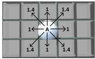
Before we start to present the specific way of optimized A* functionality, it is important to know the values associated to each direction a node can take. These values are very important, because this way we can measure the distance we traveled, so we can find the shortest path.
Figure 1. Specific cost values of each direction (next position) for the optimized A* algorithm.
The map of the environment is represented as a matrix and each space of the matrix represents a position. For every move, depending on the direction, we have a cost and for this application we have set the next values:
for going on horizontal or vertical with a unit, the cost is 1;
for going on diagonally with a unit, the cost is 1.4;
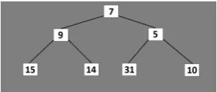
Figure 2. Examples of G, H and F cost calculation for the optimized A* algorithm.
In Fig. 2 it is presented an example of the optimized A* algorithm functionality showing the computed values for the three cost functions that were denoted by us as:
G cost: represents the cost that was calculated from the start node to the current node.
H cost: represents the estimated cost from the current node to the final node. It needs to be mentioned that the H cost doesn’t take in consideration obstacles.
F cost: represents the sum between G cost and H cost.
Also, we have denoted with A the seeker and with B the destination. At the beginning of the optimized A* algorithm application, it is checked if the position of A represents the destination too, if not, the position of A is saved in the closed vector and in the open vector are saved all the neighbors of A. In the next step, the open vector will be examined and it will take the node with the minimum F cost and A will move to that position. If in the open vector we have two or more elements with an equal F cost, the algorithm will choose the node with the lowest G cost.
We remind that the A* algorithm optimization was made about the way of searching the next position in the open vector and the way this vector is organized. At this moment, in the open vector are saved all the possible future positions of the seeker and at every iteration it is needed to examine the whole vector for finding the element with the lowest F cost. We have to note that if the environment map will become bigger or more complicated, the algorithm will be more inefficient, because the open vector will become very big and all iterations for finding the lowest F cost will take a lot of time, meaning that the time complexity of the shortest path search A* algorithm will increase significantly. In this context, we apply an optimization method to the A* strategy, in order to decrease the running time by the way of searching the next position in the open vector and the way that this vector is organized. The application of this optimization method is detailed for an example, as follows.
For an easier description, we will divide the optimization into the next steps:
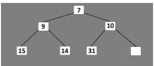
Step 1. Organize the open vector as a binary tree
having in nodes the F cost value associated to a position of the A seeker.
Thus, in step 1 it is presented the open vector in the form of a binary tree and the number associated to each element represents the F cost associated to a position (see in Fig. 3). Each new element that is introduced will be placed at the last position available in the tree. In our case, the next free position is as a right child of the node with the F cost equal to 10.
Figure 3. Illustration of step 1.
We can observe in Fig. 3 that the nodes from the tree are arranged in the order of their F cost. The root node represents the node with the lowest F cost.
Step 2. Insert in the tree (in an available position) a
new node representing the F cost of the A seeker next position.
The basic rule we are using is that none of the children nodes should have a lower cost than his parent node.
As we showed in step 1, the new node that was added was positioned in the first available position, in our case as the right child of the node with the F cost equal to 10 (see Fig. 4). We can observe that his position does not respect the rule, so we need to find the right position.
Figure 4. Illustration of step 2.
Step 3. Find the right position of the new node
inserted in the tree by sorting the tree with the heap sort algorithm.
At this step we started to search the right position for the node with the F cost equal to 5. It was checked if 5 is lower than 10 and it is true, so the position of node with the value of 5 will be switched with the node with the value 10 (see Fig. 5).
Figure 5. Illustration of step 3 – first switch.
(see Fig. 6). At this moment, our tree is sorted and is ready for the next phase.
Figure 6. Illustration of step 3 – second switch.
Step 4. Extract from the sorted tree the node with
the minimum F cost.
In this step from the sorted tree it will be extracted the node with the lowest F cost (see Fig 7). And here we can notice that finding the lowest F cost from the open vector doesn’t need any more calculations or iterations because we already know that the lowest F cost is the root of the tree. After the node extraction, the tree needs to be sorted again in the next step.
Figure 7. Illustration of step 4.
Step 5. Sort again the tree after the extraction of
the node with minimum F cost (i.e. the root node).
The tree sorting will proceed by following the next rule. The last element from the vector will be put as the node root (see Fig. 8). At this moment, all we have to do is to find the right position for the node with the value of 10, because the rest of the nodes are already sorted.
Figure 8. Illustration of step 5 – first switch from last element to root node.
The node with the value of 10 was checked if it’s higher than his two children. Because both of them are lower, it will make a comparison between them and the lower one will be the one that it will be switched with 10. In our case this node will be the node with the value of 7 (see Fig. 9).
The tree sorting will continue and it will be checked if the node with the value of 10 has children with F cost lower and we can observe that it has only one child and that has the value of 31. The tree is now sorted.
Figure 9. Illustration of step 5 – tree sorting end.
In the previous figures we can observe that we have a binary tree which it is read as a vector in the application program, but it is structured and organized as a binary tree.
Figure 10. The index of each node from the tree shown in fig. 9.
In figures 19, nodes were shown in terms of their F cost values, but every node has an index and that index represents the position in the vector (as shown in Fig. 10). For example, the node with the index equal to 0 represents the root node and the nodes with the indexes equals to 1 and 2 represents the children nodes of the root.
In order to be able to identify the children of a node, we have used the next formulas:
to identify the left child the formula is given by equation (2):
Cs = 2 * n + 1
where, Cs is the index of the left child and n
represents the index of the current node for which we want to find its right child.
For example, the left child of the node with the index equal with 2 is the following:
Cs = 2 * 2 + 1 => Cs = 5 (as in Fig. 10).
to identify the right child, the formula is given by equation (3):
Cd = 2 * n + 2
where, Cd is the index of the right child and n
represents the index of the current node for which we want to find its right child.
For example, the right child of the node with the index equal with 2 is the following:
Cd = 2 * 2 + 2 => Cd = 6 (as in Fig. 10).
In order to find the parent of a node, we have used the formula given by equation (4):
P = (n – 1) / 2 (4)
where, P is the index of the parent node and n
For example, for knowing the parent of the node 5 and the node 6 we will have:
P = (5 – 1) / 2 => P = 4 / 2 => P = 2
P = (6 – 1) / 2 => P = 5 / 2 => P = 2,5 (ignoring the decimal, we will have only 2).
As we can see in Fig. 10, the parent node of 5 and 6 it is the node with the index equal to 2.
The example that was presented in this section showed the optimization method application in detail. Synthesizing, the main contribution of our method is speeding up the search by the way of searching the next position in the open vector of the A* strategy and the type of organization adopted it.
III. APPLICATION
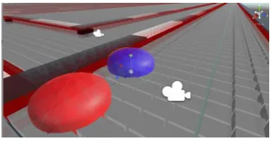
In order to prove the efficiency of our optimized shortest path search algorithm based on A* strategy we have developed an application that was integrated in an e-learning virtual environment, LearningONE [6]. LearningONE was developed in a first stage as an e-learning platform for teaching some courses from the Computer Science domain, Artificial Intelligence and Object Oriented Programming. The application was included in the Artificial Intelligence course module at the topic of informed search strategies demonstration and was built as a virtual reality simulation of A* and optimized A* application to a scenario of two virtual mobile robots that navigate in a maze and are followed by a camera.
The e-learning virtual platform, LearningONE, was developed by following the main guidelines described in [10]. Its main purpose is to provide more applications of the theoretical course subjects in order to create engaging experiences for students. This pedagogical method was adopted under the perspective of developing a blending learning system (e.g. as described in [11], [12]), which can improve students learning performances.
The software tools used for implementing the LearningONE platform and the application (virtual mobile robots navigation in a maze) are: Unity software package (for the development of the e-learning platform and virtual reality module), Blender software package (for 3D object modelling) and Microsoft Visual Studio 2017 (for the implementation of the A* algorithm and the optimized A* algorithm in the C# programming language).
Figure 11. A* algorithm demonstration development interface (in Unity).
Fig. 11 shows the interface of the A* algorithm demonstration, implemented in Unity. Fig. 12 presents a screenshot of the application interface with the A*
algorithm and optimized A* algorithm demonstration. The two virtual mobile robots are shown by the camera (in the right upper corner of the interface), during their navigation in the maze (which appear in the left side of the application interface).
Figure 12. Screenshot of the application interface with the A* algorithm and optimized A* algorithm demonstration
We have run several navigation tasks of the two virtual robots. The experimental results obtained were visible better in the case of using the optimized A* algorithm, because the optimization brings better results with more than 50% faster for the time needed to find the shortest path between two locations in the maze. Table I shows a selection of the best results obtained for the running time of the optimized A* algorithm during various experiments. These results showed that the optimized shortest path search algorithm based on the A* strategy performs faster than the A* algorithm. The performance improvement is more evident when the search space is bigger (i.e. for more complex and larger environments).
TABLE I. EXPERIMENTAL RESULTS – RUNNING TIME
Crt. No.
Running Time [ms]
Experiment A* algorithm Optimized A*
algorithm
1. Experiment 1 104 36
2. Experiment 2 105 35
3. Experiment 3 112 44
CONCLUSION
The paper described a faster shortest path search algorithm based on the A* strategy. The main optimization of the A* algorithm is related to the way of searching the next movement and the organization of the vector with the next possible movements. The performance improvement of the optimized A* search algorithm in terms of running time is more evident when the environment is much bigger and complex. The optimized algorithm was integrated in a virtual e-learning system, LearningONE, for the application of virtual mobile robot navigation in a maze, developed under the Informed Search Strategies module of the Artificial Intelligence course taught to undergraduate students from the Computer Science program of study.
algorithm based on A* strategy to a real world robot navigation problem solving.
REFERENCES
[1] S. Russell and P. Norvig, Artificial intelligence – a modern approach, Prentice Hall, 3rd edition, 2010.
[2] J. Pearl, Heuristics: Intelligent search strategies for computer problem solving, Addison-Wesley, Reading, 1984.
[3] E. W. Dijkstra, “A note on two problems in connexion with graphs”, Numerische Mathematik, vol. 1, pp. 269-271, 1959. [4] P. E. Hart, N. J. Nilsson, and B. Raphael, “A formal basis for
the heuristic determination of minimum cost paths”, IEEE Transactions on Systems Science and Cybernetics, vol. 4, pp. 100-107, 1968.
[5] P. E. Hart, N. J. Nilsson, and B. Raphael, Correction to “A formal basis for the heuristic determination of minimum cost paths”, SIGART Newsletter, vol. 37, pp. 28-29, 1972. [6] S. T. Groza, “Design and implementation of an e-learning
system integrated in a virtual world”, BSc diploma project, Petroleum-Gas University of Ploiesti, 2018.
[7] R. Dechter and J. Pearl, “Generalized best-first search strategies and the optimality of A*”, Journal of the ACM, vol. 32, pp. 505-536, 1985.
[8] H. Ma, S. Koenig, N. Ayanian, L. Cohen, W. Hönig, T. K. Satish Kumar, T. Uras, and H. Xu, “Overview: Generalizations of multi-agent path finding to real-world scenarios”, Proceedings of IJCAI Workshop Multi-Agent Path Finding, 2016.
[9] D. Delling, P. Sanders, D. Schultes, and D. Wagner, “Engineering route planning algorithms”, Algorithmics of Large and Complex Networks: Design, Analysis, and Simulation, Springer, 2009.
[10] B. Holmes, J. Gardner, and M. Gamble, “e-Learning: Concepts and practice”, Journal of Pedagogic Development, 2006.
[11] J. Bersin, The blended learning book, San Francisco, John Wiley, 2004.