Historical Impulse Response of Return Analysis Shows Information
Technology Improves Stock Market Efficiency
William Leigh
University of Central Florida College of Business Administration PO Box 161400
Orlando, FL 32816-1400, USA
E-mail: [email protected]; http://www.bus.ucf.edu/leigh/
Russell Purvis Clemson University
College of Business & Behavioural Science 165 Sirrine Hall
Clemson, SC 29634, USA
E-mail: [email protected]; http://people.clemson.edu/~rlpurvi/
Keywords: empirical impulse response function, impact of information technology, market efficiency, information diffusion, econophysics, stock market as information system
Received:March 9, 2007
We compare average impulse response of rate of return curves computed from more than sixty-seven years of historical Dow Jones Industrial, Transportation, and Utility Average closing values. The curves are relatively consistent in shape until the 1990s, when marked changes, indicative of improved market efficiency, occur for the Dow Jones Industrial Average. We argue that the effect is a result of the increased availability and reduced cost of online stock trading and of the more rapid dissemination and diffusion of information made possible by information technology. The basis for this argument is that: 1) the effect occurs only for the Industrial Average, which is comprised of stocks which are most well-known to the investing public, and not for the Transportation or Utility Averages, which are comprised of less well-known stocks; and 2) the effect is progressive and contemporaneous with the growth of the use of personal computing and the internet.
Povzetek: Z analizo prejšnjih dogajanj je pokazano, da informacijske tehnologije izboljšujejo učinkovitost borz.
1 Introduction
The output signal response from a continuous system to a narrow pulse input signal is the system’s impulse
response. Physical systems may be analyzed by
observing the system’s response to a sharp input, by striking a bell, for example, and observing the movement of points on the surface of the bell. Economic systems are not amenable to the sort of laboratory analysis that may be applied to physical systems, but an investigator of the stock market may detect narrow pulses of increased (or decreased) rate of return in the time series of daily rates of return for the stock market and then observe the behavior of the subsequent daily returns, thus employing a synthetic impulse response analysis.
The assumption of market efficiencyis important in the theory of the academic discipline of Finance. A perfectly efficient market adjusts its prices to new information instantaneously and correctly. This implies that for a perfectly efficient market, all relevant information available in the past history of stock price as
well as any newly revealed information is considered and reflected in the current price, and this means that historical price information alone may not be used to forecast future prices with any useful degree of success. Perfect market efficiency requires the instantaneous availability and instantaneous correct application of perfect information by all market participants, and these assumptions are not true in the real world of the stock market. Thus, as friction is assumed to be negligible in order to consider an ideal “F=MA”, the effects of investor psychology and of instantaneous and non-homogeneous information communication and application are assumed to be negligible by the assumption of a perfectly efficient market. Brynjolfsson and Smith (2000) consider internet retail as a “frictionless” commerce.
may not be truly efficient, but perfect efficiency is a benchmark by which we can evaluate how well a market serves society. Perfect stock market efficiency is a worthwhile ideal, though perfect market efficiency is impossible. Kauffman and Walden (2001) identify the effect of the widespread use of modern information technology on market efficiency as a topic for future study.
Successes with the application of theory and techniques from physics, such as impulse response analysis, to understanding and predicting the behavior of the stock market are reported primarily in the physics journals (for example, Sornette and Zhou 2006). There are some reports in the economics and finance journals of the use of techniques from physics for modeling economic and financial systems (for example, Sornette and Zhou 2005), but as most academics in economics and finance hold to the assumption that the stock markets are perfectly efficient, and as the physics models tend to be useful only in modeling markets which are not perfectly efficient, the physics journals (where this work is sometimes called “econophysics”) are a more likely place to find the application of physics models to the stock markets than are the economics and finance journals.
Donella Meadows (1999) identifies “leverage points”, places to intervene in a system to effect change. These leverage points are, in increasing order of effectiveness:
Constants, parameters. Sizes of buffers and stocks.
Structure of material stocks and flows. Lengths of delays.
Strength of negative feedback loops.
Gain around driving positive feedback loops. Structure of information flows (who does and
does not have access to what kinds of information.)
Rules of system.
Power to add or change the system structure. Goals of the system.
Mindset out of which the system arises. Power to transcend paradigms.
The introduction of innovations in the stock market system is ongoing and continuous (White 2003). The behavior of the stock market may be affected by changes in the structure of the market itself, in the form of new products and new regulations, or by changes in the information systems used by the market participants. Offering new stock market products constitutes level 10 leverage point change to the stock market system. New regulations, including the spate of new regulations enacted after the 1987 Crash (Lindsey and Pecora 1998), are examples of leverage point change no more powerful than level 8. The increased availability and reduced cost of online stock trading and the more rapid dissemination of information, all made possible by the personal computer and internet information technology revolution,
constitute more powerful level 6 change at least, and may involve change as powerful as level 4. “Day trading”, enabled by information technology, may constitute change as strong as level 2.
Diffusion models are used to model the adoption of innovation, and this is well-studied; Rogers (1983) is a seminal survey. Physicists model radiation, dispersion, and diffusion phenomena, as surveyed in Beltrami (2002): for example, Frick’s Law of Diffusion, Newton’s Law of Cooling, Fisher’s Equation. These models from physics may be applicable to information diffusion in the stock market system. Houthakker and Williamson (1996) survey the research concerning the characteristics of the stock market traders’ information medium and how these characteristics may affect the diffusion of information. Surowiecki (2004) surveys the research explaining how markets can arrive at correct prices and can be efficient if the market participants receive timely information.
An impulse response of return graph may be constructed with rate of return for a period (40 trading days in this study) in the vertical axis and time in the horizontal axis. If there is no persistence of the effect of the impulse, then the average impulse response of return behavior for the period is “flat”, in graphical terms, after the impulse, and we may say that the market is perfectly efficient. If the graph is not flat then the market is not perfectly efficient.
Change in price in the stock market is the effect of information on the traders’ value estimates for the stocks. Lags in the diffusion and adoption of new information can explain non-flat response of return behavior. Using the terminology of the innovation diffusion literature, “early adopters” may receive information early and act quickly, while “late adopters” may receive new information late and/or act slowly.
2 Method
The results in this paper are from the use of a method for deriving an empirical impulse response function of return, such as is discussed in Koop et al (1996). The method is applied to rolling 5000 trading day intervals of closing values of three Dow Jones Averages (Industrial --DJIA, Transportation -- DJTA, and Utility -- DJUA) for the period 5/28/1936 to 1/26/2004, which comprises 17,000 trading days.
For each trading day t, a return, rt, is computed, which is the change in closing price over the 40 trading days following as a fraction of price, pt. Next we determine a trading day history window for ptsuch that pt
is not included in calculating return values for prices in that history window. Since any return for trading days t-40through tincludes ptin the calculation, a 400 trading day history window preceding trading day tthat does not include ptwould begin at day a = t-400-40 = t-440 and end at day b = t-40-1 = t-41. This presentation uses 40 trading days as the return horizon and 400 trading days as the history period throughout.
Hence we have:
pt= closing value of Dow Jones Average on trading
day t
rt= ( pt+40
–
pt) / pt return for trading day tRa,b= { rt| a ≤ t ≤ b } a set of returns for trading days
a to b
Rt-440,t-41 = { rt| t-440 ≤ t ≤ t-41 } Historical Return
Set for pt
A positive impulse is identified if a return, rt, exceeds the average of the returns in pt’s historical return set Rt-440,t-41by a multiple of the standard deviation of the returns in that historical return set. A value of 1.5 is used for this multiplier throughout this paper.
řt= 1/n∑ⁿk=1rk the average return for the historical
return set, Rt-440,t-41
st= √[1/n-1∑ⁿk=1(rk-řt)2] the standard deviation for
the historical return set, Rt-440,t-41
m = 1.5 a constant multiplier
it= 1, if rt> řt+ m•st the impulse for trading day t
0, otherwise
Table 1 contains the beginning and ending trading day numbers and the corresponding dates for the intervals used. For each interval the table lists the number of positive impulses which occurred in that interval for each of the three Dow Jones Averages.
Begin End Begin End DJIA DJTA DJUA 36-56 1 5000 05/28/36 05/21/56 415 427 395 56-76 5001 10000 05/22/56 05/03/76 376 528 500 60-80 6001 11000 05/11/60 04/17/80 409 522 491 64-84 7001 12000 05/04/64 03/30/84 469 496 481 68-88 8001 13000 04/24/68 03/16/88 541 510 507 72-92 9001 14000 05/16/72 02/28/92 497 466 477 76-96 10001 15000 05/04/76 02/13/96 514 446 441 80-00 11001 16000 04/18/80 01/31/00 525 393 458 84-04 12001 17000 04/02/84 01/26/04 470 378 521
Trading Day Date
Interval Impulses
Table 1: Intervals used in terms of trading days and the number of impulses in each interval for each Dow Jones Average.
The method defines the “response” to the impulse in terms of time lags expressed in trading days. This impulse response function is derived from an aggregation of trading days in a response set. Returns for trading days are identified for inclusion in the impulse response return set by relating them to the return for the trading day preceding them by a lag of between 1 and 200 trading days. If a trading day’s return is identified as a return associated with an impulse, then the lagged trading day
return is a member of the response set. There is an impulse response return set, Ia,b,L, for each of the 200 lag values for trading day interval from ato b.
That is, we have:
L = 1,…, 200 the lag in trading days
Ia,b,L= { rk | ik-L = 1 and a ≤ k ≤ b } the impulse
response return set given L from trading day a to trading day b
ǐa,b,L= 1/n∑ⁿk=1 rk where rk is in Ia,b,L the average
impulse response return in Ia,b,Lfor lag L
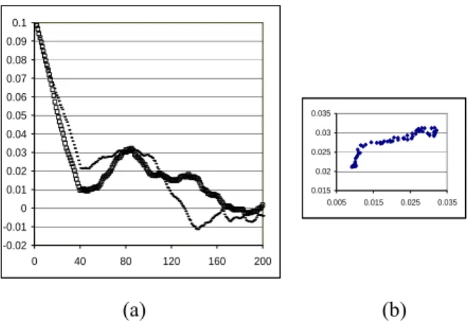
Figure 1(a) shows a graph of impulse responses for the time intervals 36-56 (the 200 ǐ1,5000,L values for the
years 1936 to 1956, denoted by the squares in the graph) and 56-76 (the 200 ǐ5001,10000,Lvalues for the years 1956 to
1976, denoted by dashes) for lags of 1 to 200. Figure 1(b) graphs the impulse response values for interval 36-56 on the x-axis and interval 56-76 on the y-axis for lags of 40 to 100. The method is ex-ante for lags of 40 and up, and so it is the impulse responses for those lags that are of interest for forecasting and trading applications.
-0.02 -0.01 0 0.01 0.02 0.03 0.04 0.05 0.06 0.07 0.08 0.09 0.1
0 40 80 120 160 200 0.015
0.02 0.025 0.03 0.035
0.005 0.015 0.025 0.035
(a) (b)
Figure 1: (a) Impulse response graphs for intervals 36-56 (squares) and 56-76 (dashes) for lags 1 to 200. (b) Graph of impulse response values for interval 36-56 against impulse response values for interval 56-76 for lags of 40 to 100.
3 Historical comparison
Table 2 shows correlation coefficient values calculated for each interval, for each of the three Dow Jones Averages, for lags 40 to 100, and for lags 40 to 200. The correlation coefficient is calculated for the impulse response curve for interval 36-56 for the respective Dow Jones Average as correlated against each of the other intervals for the same Dow Jones Average. The correlation coefficients then are:
cX,Y = correlation coefficient as computed from
the sets X and Y of values paired as (xL,yL)
Ca,b,c,d,L1,Ln = correlation coefficient as computed from c ǐa,b, ǐc,d( { ǐa,b,L | L1≤ L ≤ Ln}, {
ǐc,d,L| L1≤ L ≤ Ln} )
For example, the top value in the second column of Table 2 is 0.907. This is the evaluation of
C1,5000,5001,10000,40,100 for the Dow Jones Industrial Average.
40-100 40-200 40-100 40-200 40-100 40-200 56-76 .907 .734 .434 .627 .654 .385 60-80 .943 .700 .667 .547 .376 .161 64-84 .923 .765 .661 .594 .343 .298 68-88 .910 .805 .700 .642 .334 .269 72-92 .863 .751 .600 .498 .077 .235 76-96 .893 .828 .490 .215 -.125 .124 80-00 -.496 .706 .330 .426 .355 .276 84-04 -.475 .391 .490 .026 .617 .301
DJIA DJTA DJUA
Interval
Table 2: Correlation coefficient values for the impulse response function of each interval correlated with the first interval 36-56 for each Dow Jones Average.
The correlation coefficient is useful for comparing the impulse response curves in a rough-and-ready way. In Table 2 it may be seen that the correlation coefficient values for lags 40 to 100 change markedly in sign and magnitude for the DJIA for intervals 80-00 and 84-04 as compared with the correlation coefficient values for the intervals which went before. Note the negative correlation values for the Industrial Average in the last two rows of Table 2.
Table 3 is prepared in a similar way to Table 2 except that the 36-56 interval for the Dow Jones Industrial Average is used as the correlation partner for each of the other intervals (instead of the 36-56 interval in the respective Dow Jones Average.)
40-100 40-200 40-100 40-200
56-76
.426
.816
.953
.217
60-80
.850
.812
.865
.203
64-84
.875
.827
.865
.395
68-88
.970
.895
.870
.459
72-92
.927
.727
.718
.557
76-96
.803
.537
.600
.683
80-00
.581
.594
.861
.749
84-04
.714
.367
.938
.609
DJTA
DJUA
Interval
Table 3: Similar to Table 2 but 36-56 interval for DJIA is used as correlation partner for each of the intervals in the DJTA and in the DJUA.
In Table 3 the correlation coefficient values are generally higher for the DJTA and DJUA than they are in Table 2. The correlations continue to be relatively strong through the 80-00 and 84-04 intervals.
Figure 2 shows graphs of the impulse response functions for all of the intervals for the DJIA, except that the curves are offset by the average profit in each of the intervals. Thus, on the y-axis Figure 2 shows excess profit, which is the difference between ǐa,b,L, the average
impulse response return in the set Ia,b,Lfor trading days a to b and for lag L, and the average of returns from trading days a to b, that is the set Ra,b. A market timing rule which would have worked before 1990 on the DJIA and still worked on the DJTA and DJUA to the end of the study: “Buy at impulse lag day 80 and sell after holding for 40 days”.
-0.02 -0.01 0 0.01 0.02 0.03
40 80 120 160 200
Figure 2: Impulse response for DJIA for each interval, adjusted by average profit in interval. Values for interval 36-56 are denoted by the square, for interval 80-00 by “+”, and for interval 84-04 by “x”.
4 Conclusion
The stock market acts like an elastic medium in time which transmits shock waves, in this case for rate of return shocks. The impulse response behavior of the stock market information transmission medium was relatively homogeneous from 1936 up until about 1990. In Figure 2, an oscillating wave is seen, with over-reaction and under-over-reaction out to 200 days. About 1990, the stock market price information transmission medium changed drastically for the DJIA, with the response from the shock dampened out immediately. No similar dampening is seen for the DJTA and DJUA, though perhaps we can expect the DJTA and DJUA to be transformed in the same way in the future.
contemporaneous with this revolution in information technology and that the effect is pronounced in the case of the stocks most widely known and traded by the segment of the stock trading population which has been newly empowered by the information technology revolution leads us to make the argument that the effects are primarily the result of information technology.
This work investigated a trading horizon of 40 trading days. An objective of future work will be to determine the effect on impulse response of information technology through the full spectrum of trading horizons, from 1 day to 100 days or more. An interesting hypothesis, consistent with the idea that the technology and the traders use of it become more effective as time goes on, is that the “flattening” begins at the longer trading horizons and over time, progresses, to the shorter trading horizons.
References
[1] Beltrami, E. (2002). Mathematical Models for Society and Biology. Academic Press, San Diego. 199 pages.
[2] Brynjolfsson, E. and M. Smith (2000). Economics and electronic commerce: survey and research directions. International Journal of Electronic Commerce, 5(4), 5-117.
[3] Houthakker, H.S. and P.J. Williamson (1996). The
Economics of Financial Markets. Oxford
University Press, Oxford. 361 pages.
[4] Kauffman, R.J. and E.A.Walden (2001).Economics and electronic commerce: survey and research directions. International Journal of Electronic
Commerce.5(4), 5-117.
[5] Koop, G., M.H. Pesaran and S.M. Potter (1996). Impulse response analysis in nonlinear multivariate models. Journal of Econometrics, 74(1), 119-148. [6] Lindsey, R.R. and A.P. Pecora (1998). Ten years
after: regulatory developments in the securities markets since the 1987 market break. Journal of Financial Services Research, 13(3), 283-314. [7] Meadows, D. (1999). Leverage Points Places to
Intervene in a System. The Sustainability Institute, Hartland, Vermont. 19 pages.
[8] Rogers, E.M. (1983). Diffusion of Innovations. The Free Press, New York. 453 pages.
[9] Sornette, D. and W Zhou (2005). Non-parametric determination of real-time lag structure between two time series: the "optimal thermal causal path" method. Quantitative Finance,5, 577-591.
[10] Sornette, D. and W Zhou (2006). Importance of positive feedbacks and overconfidence in a self-fulfilling Ising model of financial markets. Physica A: Statistical and Theoretical Physics,370(2), 704-726
[11] Surowiecki, J. (2004). The Wisdom of Crowds. Doubleday, New York. 296 pages.
[12] White, L.J. (2003). Technological change, financial innovation, and financial regulation in the U.S.: the challenges for public policy. In G. Constantinides, M. Harris, and R.M. Stulz (Ed.), Economics of