Uniform Fractional Part: A Simple Fast Method for Generating Continuous Random Variates

(1)

Uniform Fractional Part: A Simple Fast Method

for Generating Continuous Random Variates

H. Mahlooji

1;

_{, A. Eshragh Jahromi}

1

_{, H. Abouee Mehrizi}

1

_{and N. Izady}

1

A known theorem in probability is adopted and through a probabilistic approach, it is generalized to develop a method for generating random deviates from the distribution of any continuous random variable. This method, which may be considered as an approximate version of the Inverse Transform algorithm, takes two random numbers to generate a random deviate, while maintaining all the other advantages of the Inverse Transform method, such as the possibility of generating ordered as well as correlated deviates and being applicable to all density functions, regardless of their parameter values.

INTRODUCTION

Random variate generators are at the heart of any stochastic simulation. Generating samples from a di-verse variety of distributions has become an established research area since World War II, when the feasibility of performing Monte Carlo experiments became a reality. The generation of non-uniform random deviates has come a long way, from methods dating back to a time prior to the era of the computer [1] to the latest novel methods, such as the Ziggurat and vertical strip [2]. While some methods are general in nature, some others are intended for a particular distribution.

Fishman [3] summarizes the milestones in the development of this eld as follows: In 1951, von Neumann showed how \principles of conditional prob-ability could be exploited for generating variates". In 1964, Marsaglia et al. demonstrated how \a synthesis of probabilistic and computer science considerations could lead to highly ecient algorithms" and, nally, in 1974, Ahrens and Dieter showed how \a bounded mean computing time could be realized for an arbitrary distribution".

Among the algorithms developed so far, some are widely used and/or are more ecient than others. For instance, while the Inverse Transform method is quite simple, if the desired cumulative distribution function cannot be expressed in a closed form, one has to resort to numerical methods, which signicantly decrease

1. Department of Industrial Engineering, Sharif University of Technology, Tehran, Iran.

*. To whom correspondence should be addressed. E-mail: [email protected]

the eciency of the algorithm. If the distribution function can be stated as a convex combination of other distribution functions from which, perhaps, it is easier to generate values, the Composition method would be a competitive alternative. While these methods deal directly with the intended distribution itself, the Acceptance Rejection method targets a majorizing or hat function instead of the given density. The eciency of this method is directly related to the chosen hat function, where identifying a `perfect' hat function in each case has always posed as an elusive goal. There are many other algorithms in the literature, such as: Forsythe-von Neumann's Ratio of Uniforms and the like, which all can be found with in-depth analysis and examples in Devroye [4] or Fishman [3]. Hormann [5] proposed a method named the Transformed Density Rejection that can be applied to all distributions. This is a complex method and is usually time-consuming when it comes to nd the hat and the squeeze functions. Some other universal random variate generators, such as the Strip method, have also been discussed thor-oughly in Hormann et al. [5,6].

One of the most dicult problems in random variate generation is selecting an appropriate well-suited algorithm. Devroye [4] suggests speed, set-up time, length of compiled code, range of set of applications and simplicity as the factors for evaluating dierent methods. Law and Kelton [7] add exactness and robustness to this list. Exact algorithms generate variates according to the desired distribution, with the assumptions of availability of a perfect random number generator and the computer capability to store real numbers, while approximate methods need more assumptions. Robustness deals with the eciency of

(2)

the algorithm over the entire range of distribution parameters.

In this article, a method is presented, which is applicable to the distributions of all continuous random variables. Although this algorithm belongs to the approximate category, its simplicity, speed, robustness and coverage make it a powerful competitor against exact methods, while its accuracy can be enhanced to almost any desired level. This method, which can be looked upon as a piecewise linear approximation generator, demands a rather high cost of set-up time, in the case of a rare event simulation. An added set-up time is expected also for cases when the density is somehow changed during the simulation run.

The structure of this paper is as follows: First, there will be a discussion on theoretical considerations when developing the probabilistic interpretation of the Uniform Fractional Part (UFP) method. Then, the dependence issue between the random numbers used as input to the algorithm will be elaborated on and the initial algorithm will be presented. After that, Simplications to the initial algorithm are included and computational results are presented. Finally, the paper ends with concluding remarks and suggestions for further developments.

THEORETICAL BASIS OF THE UFP METHOD

The uniform fractional part method is based on the following theorem, which appears as an exercise on page 72 in Morgan [8]:

Theorem 1

Suppose X and U1to be two independent uniform [0; 1]

random variables. Then, U2, dened as:

U2= U1+ X bU1+ Xc ; (1)

is uniformly distributed over the interval [0; 1], where bc stands for the \largest integer smaller than, or equal to ".

There is an interesting extension to this problem (see [8] p. 72). If the continuous random variable, X, follows any distribution other than uniform [0; 1], U2is

still distributed uniformly over the interval [0; 1]. It is tempting to infer that, based on Equation 1, one can generate values for the continuous random variable, X, with the use of two uniform random numbers, such as U1 and U2. Following this notion,

one can isolate X in Equation 1 to get:

X = U2 U1+ bU1+ Xc : (2)

Since U1 takes values between 0 and 1, then bU1+ Xc

is equal to either bXc or bXc + 1. This means that one of the following two cases is relevant:

a) If bU1+ Xc is equal to bXc, Equation 2 simplies

to:

X = U2 U1+ bXc : (3)

Since the fractional part of X (i.e., X bXc) falls between 0 and 1, one can write:

0 X bXc = U2 U1 1

) U1 U2 1 + U1) U2 U1: (4)

b) If bU1+ Xc is equal to bXc + 1, Equation 2 takes

the following form:

X = U2 U1+ bXc + 1: (5)

Since the fractional part of X falls between 0 and 1, one can write:

0 X bXc = U2 U1+ 1 1

) U1 1 U2 U1) U2 U1: (6)

Thus, Equation 2 can be rewritten as follows: X =

(

U2 U1+ bXc ; U2 U1

U2 U1+ bXc + 1; U2< U1 (7)

All this means that, in generating deviates for any continuous random variable X, three values are needed: U1, U2 and bXc. U1 and U2 are easily provided by

random number generators, such as the one developed by Marsaglia and Tsang [9]. To generate values for bXc, one can use the Inverse Transform method. In fact, suppose X FX. If one assumes that X takes

non-negative values only, then:

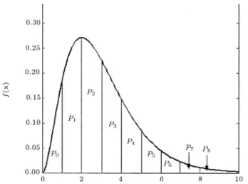
pi= P (bXc = i) = P (i X < i + 1)

= FX(i + 1) FX(i); i = 0; 1; 2; (8)

Hence, bXc has a discrete distribution and takes value i with probability pi, as illustrated in Figure 1, for an

arbitrary distribution. Nowadays, one can easily have access to sources that provide very accurate values of pi

for any density function once the mesh points, bXc = i, are specied. This obviously can also be done for the special case of pi = p, such that P

8ipi = 1:0 always

holds. Now, the following algorithm can be proposed. Algorithm 1

1. Generate U1 and U2 as two independent uniform

[0; 1] random numbers, 2. Generate a value for bXc,

(3)

Figure 1. Probabilities associated with bXc.

[0; 1] random numbers, 4. Generate a value for bXc,

5. If U2 U1, then, X = U2 U1+ bXc; otherwise,

X = U2 U1+ bXc + 1.

This algorithm works exactly, provided that U1

and U2 in Equation 1 are independent. In fact, if

X U[m; n], it can be easily shown (see the Appendix for the case of integer m and n) that U1 and U2

are independent. However, as will be investigated in detail, this is not true in general. Hence, in cases where U1and U2do not behave as independent random

variables, this algorithm can be modied and used as an approximate method toward generating random deviates. This matter is discussed in following sections. Up to this point, all this method does is randomly to select one of the integer values within the range of X(one of the columns in Figure 1) and then adds U2 U1 to it, to make a random deviate. Obviously,

it is quite restrictive if one is to select only integer values for X as the mesh points. So, Theorem 1 is now generalized in such a way that once needed any set of non-equidistant real values within the range of X can also be chosen and implemented in the algorithm. To achieve this purpose, rst, the following denition is presented.

Denition 1

The operand, Int, is dened as: Int (X + ) =

(

ai; X + < ai+1

ai+1; X + > ai+1 (9)

where X is a continuous random variable taking values in the interval [ai; ai+1) and a0is are distinct real values,

such that ai< ai+1; i = 1; 2; .

Theorem 2

Suppose X is any continuous random variable and ( 1; a1), [a1; a2); ; [ak; 1) is a nite partition of

the range of X. Now, dene A as the set of mesh points, i.e., A = fa1; a2; ; akg. Also, dene di as

the distance between two successive members of A, as di = ai+1 ai, i = 1; 2; ; k 1. Given that U1 is a

uniform [0; di] random variable for any value of i, when

X takes a value in an interval of the form [ai; ai+1),

then, U2 dened as:

U2= U1+ X Int (X + U1); (10)

is uniformly distributed over the interval [0; di].

To prove Theorem 2, the following lemma is rst presented.

Lemma 1

Given that di2 <+, x 2 < and y 2 [0; di] are constant

real numbers and U 2 [0; di) is a real variable for i =

1; 2; ; k 1, then the following equation:

x + U Int (x + U) = y; (11)

has one, and only one, solution, such as U = u. Proof

First, it is shown that Equation 11 will always have an answer. If U is isolated in Equation 11, one will arrive at:

U = y + Int (x + U) x: (12)

It is obvious that, for any particular i, Int (x + U) is either equal to Int (x) or Int (x) + di. So, Equation 12

can be presented as one of the following two cases: - If Int (x + U) = Int (x), then, U = y + Int (x) x )

u = y + Int (x) x,

- If Int (x + U) = Int (x) + di, then, U = y + Int (x) +

di x ) u = y + Int (x) + di x.

Thus, one answer always exists. If there were two dierent solutions as:

u1= y + Int (x) x;

and:

u2= y + Int (x) + di x;

one would have:

0 u1< di) 0 y + Int (x) x < di

) di y + Int (x) + di x < 2di

(4)

which contradicts the assumption of 0 u2 < di. A

similar argument holds for u1. Hence, Equation 11 will

always have a unique solution, like U = u.

Now, based on Lemma 1, an eort will be made to prove Theorem 1. Bearing in mind that, for the case of any continuous random variable like X one can write:

P (X = x) = P

lim

h#0x X < x + h

= lim

h#0P (x X < x + h) = limh#0h:fX(x)

) fx(x) = P (X = x)_h :

One can nd the density of U2 conditioned on the

interval in which X falls as: PrfU2= u2jX 2 [ai; ai+1)g

= PrfX + U1 Int (X + U1)

= u2jX 2 [ai; ai+1)g

= Z _a_i+1

ai

PrfX + U1 Int (X + U1)

= u2jX = x;

X 2 [ai; ai+1)gd(PrfX xjX 2 [ai; ai+1)g)

= Z _a_i+1

ai

Prfx + U1 Int (x + U1)

= u2g_{PrfX 2 [a}fX(x)

i; ai+1)gdx: ₍₁₄₎

By considering Lemma 1, which states that Equa-tion 11 always has the unique soluEqua-tion, U = u, Equation 14 simplies to:

PrfU2= u2jX 2 [ai; ai+1)g

= Z _a_i+1

ai

P fU1= u1g_{PrfX 2 [a}fX(x)

i; ai+1)gdx:₍₁₅₎

Now, suppose h is a small positive value, then: PrfU2= u2jX 2 [ai; ai+1)g

= _{PrfX 2 [a}1

i; ai+1)g

Z _a_i+1

ai

(hfU1(u1))fX(x)dx

= 1

djPrfX 2 [ai; ai+1)g

Z _a_i+1

ai

hfX(x)dx

= h_d

i : (16)

So, one has:

P (U2= u2jX 2 [a1; ai+1))

h =

1 di

) fU2(u2jX 2 [ai; ai+1)) =

1

di; (17)

when h ! 0. Therefore, U2 is uniformly distributed

over the interval [0; di] and Theorem 2 is proved.

Note that, if A consists of integer values, Int (x) will result in the same values as bXc and Theorem 1 becomes a special case of Theorem 2, with di = 1,

i = 1; 2; ; k 1. In general, Equation 8 takes the form:

pi= P (Int (X) = ai) = P (ai X < ai+1)

= FX(ai+1) FX(ai); i = 1; ; k 1: (18)

In analogy to Algorithm 1, one will arrive at the following Algorithm.

Algorithm 2

1. Generate a value for Int (X) and determine the value of i;

[0; di] random variates, where didenotes the length

of the interval into which X falls;

3. If U2 U1, then X = U2 U1+ Int (X), otherwise

X = U2 U1+ Int (X) + di.

Algorithm 2 relaxes the restriction of using only integer values for X. As will be discussed later on, this would help signicantly when U1 and U2 show strong

dependence.

INVESTIGATING THE DEPENDANCE

BETWEEN U1 AND U2

Investigating the nature of the relation between the uniformly distributed random variables, U1 and U2,

can be quite intriguing. To address this issue, rst, the authors resort to a number of experiments in which they initially assume a uniform partition of the range of X and, hence, a constant mesh size di = d; 8i. For

the sake of experiments presented here, it is assumed that X is distributed according to Gamma (Figures 2, 3, 4 and 6) or Normal (Figure 5). Then, by Monte Carlo sampling on a computer, samples of arbitrary size are generated from distributions of the independent random variables, U1 and X. Each time a pair of

values (u1; x) is generated, the value u2 is computed

according to Equation 9. In this way, a sample of size, say, n, is generated for (U1; U2). By plotting the

(5)

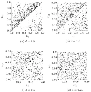
Figure 2. Scatter diagrams for (U1; U2), d = 1 and X

exponential ().

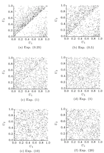
can make some interesting observations. As can be seen in Figure 2, for a uniform spacing with d = 1, when dispersion in the distribution of X is small, clear patterns between U1 and U2 can be observed in each

plot, such that it can be concluded that U1 and U2

are not behaving independently. Figure 3 displays the same behavior for d = 1:5. Figure 4 shows that instead of increasing the dispersion one can dene a more compact set of mesh points (i.e., decreasing the value of d), in order to make the patterns fade away. When one considers other distributions for the random variable X and manipulates the parameter(s) of each distribution with the aim of increasing the dispersion, similar observations are made (Figures 5 and 6). At this point, it is tempting to loosely interpret a `no visible pattern' situation as indicative of the independence of U1 and U2on [0; d]2.

Even though such experiments shed light on the dependence structure of U1 and U2, it was decided

that it would be more convincing if one were somehow able to measure the dependence between U1 and U2.

There are several correlation notions in the statis-tics literature, such as the Pearson linear correlation, Spearman's and Kendall's . All these measures have

Figure 3. Scatter diagrams for (U1; U2), d = 1:5 and X

exponential ().

a substantial drawback for the purposes of this paper: Being zero does not necessarily imply independence between the random variables involved. Devroye ([4], page 575) introduces a good measure of dependence for continuous marginals, which, for the special case at hand, is dened as:

L = 1₂ Z

jf(u1; u2) f1(u1)f2(u2)jdu1du2; (19)

where f1 and f2 are marginal densities of U1 and

U2, respectively, and f(u1; u2) stands for their joint

density function. The fact is that, if this measure of dependence between two random variables is zero, then the random variables are independent and, conversely, if the random variables are independent, then L = 0 holds true. Thus, U1 and U2 are independent if,

and only if, L = 0. In cases where L cannot be found explicitly, one can try to calculate its unbiased estimator, based on a sample of size n composed of observations such as (u1i; u2i), through the following

(6)

Figure 4. Scatter diagrams for (U1; U2), dierent values

of d and X exponential (0.25).

normal (10; 2_).

^L = 1_nXn

i=1

max

0; 1 f1_f(u(u1i)f2(u2i)

1i; u2i)

; (20)

where f1, f2 and f(u1; u2) are estimated via methods

such as Kernel Density Estimation [5].

For special cases, where X is exponentially dis-tributed with mean and for an arbitrary partition of the range of X, this measure of association has been derived and has been shown to be equal to:

Gamma (; 1).

L =

(dipi 2pi(ln(di) ln()+1 ln(pi)) +2aipi+die (ai+di)

_+e ai_d_i₎

2pidi ;(21)

given that X falls in an interval of the form [ai; ai+1),

pi is dened as in Equation 18 and di is dened as in

Theorem 2. The plot of L versus dierent values of and di is presented in Figure 7. It is observed that L

tends to zero as goes to innity or as di approaches

zero.

Note that, because of the diculty in deriving L, or even estimating it when X follows other com-mon distributions, other means were relied upon to justify the conditions under which U1 and U2 could

be considered as independent random variables. For

(7)

instance, since, when the joint density of U1 and U2

is uniform on the unit square, then U1 and U2 will

be independent (see, e.g. [4] p. 576). The following hypothesis has been tested by using the chi-square statistic for dierent densities and a wide range of their parameter values. For this purpose, when d = 1, the unit square was divided into 100 squared cells of equal area and, each time, samples of 1000 (u1; u2)'s were

generated, as described above. The dierence between the expected and observed number of points in each cell was calculated through the 2 ₌ P10

i=1 10

P

j=1

(yij 10)2

10

statistic, where yij stands for the number of observed

points actually falling inside the (i; j) cell. In this way, one will have a chi-square statistic with 99 degrees of freedom.

(

H0: f(u1; u2) = 1

H1: Otherwise (22)

Based on the values taken by the test statistic, the null hypothesis may not be accepted at rst. But, by gradually increasing the dispersion of the density of X and by feeding the same streams of random numbers to generate values for U1 and X, the values assumed

by the test statistic improved to a point where H0

could no longer be rejected. Increasing the dispersion even further, only amounts to accepting H0 by

ever-increasing p-values. These results were in line with the initial notion that `to reach the needed independence of U1 and U2, one can increase the dispersion in the

density of X either by increasing the variance of X or by expanding its range (like in the case of beta distribution)'. When the mesh size, di, assumes any

xed value other than 1, quite similar results are obtained from experimenting within the di square,

[0; di]2. In the case of varying di, still the same behavior

can be observed, except that now, the patterns of (u1; u2) must be studied in, at most, k 1 squares,

[0; di]2, i = 1; ; k 1.

Even though Figure 7 suggests that, for the case of X as a negative exponential distribution, one can treat U1 and U2 as independent random variables

when the mean of X actually tends to innity, from a practical point of view, however, one can work with very moderate values of E(X) = (values as low as 8 or 9) and yet expect to generate quite satisfactory results. In the following section, among others, the mechanism of dening values for ai's (and hence di's) are discussed,

which can almost `assure' us of the independence of U1

and U2.

SETTING UP THE ALGORITHM

The most notable task in setting up the algorithm deals with dening the set of mesh points a1; ; ak.

The mesh points are obviously dened once an ar-bitrary partition of the range of X is formed. In general, the partition can be presented as ( 1; a1],

[a1; a2); ; [ak; + 1). In case the range of X is

bounded, as a1 X ak, the partition simplies to

[a1; a2), [a2; a3); ; [ak 1; ak]. From a practical point

of view, in order to implement the UFP method, one has to cut o the range of X at one or both ends, if the range is open on one or both sides. In other words, in the case of an open range, one needs to substitute X ak, X a1 or X 2 < by a1 X ak.

This amounts to discarding a segment in the partition that includes either ( 1; a1] or [ak; +1) or both with

corresponding area(s) p0and/or pk. Depending on the

probability associated with the discarded interval(s), one should expect a serious or mild deciency in the generation of tail values by the algorithm. It is only logical that a1and/or akmust be chosen in such a way

that the risk of such deciency becomes negligible. By resorting to experimentation, it has been noted that the cut o value(s) a1 (and ak) must be selected in such a

way that p0(and pk) does (do) not exceed 0.001. This

threshold is suggested as a maximum only.

Once end points a1 and ak are given or decided

upon, points a2; ; ak 1must also be dened. Among

dierent available ways, only the `uniform probability partition' scheme is discussed. This is the alternative that makes the areas of all segments equal (i.e., p1 =

p2 = = pk 1 = p, where p is equal to _{k 1}1 ).

Following this rule, if k = 11, for instance, the mesh points will be a1; a2; ; a11 and there will be ten

segments each with an associated probability of 0.1, except, possibly, the very rst and/or the very last segment(s), depending on the necessity of a cuto operation on the left and/or the right extreme(s) of the range of X.

By choosing very small values for p, the accuracy of the UFP method will become quite acceptable. In fact, as p ! 0, the accuracy of the UFP method approaches the accuracy attainable by the Inverse Transform method when the latter is applicable. By adopting a uniform probability partition of the range of X and in light of Step 1 in Algorithm 2, one just needs to generate a random number, such as U0_,

divide it by the chosen value of p and identify index i = 1; ; k 1 as the integer part of U0

p + 1, which,

in turn, identies Int (X) = ai. In this way, the rst

step in Algorithm 2 is executed without any need for a formal search routine.

SIMPLIFYING THE ALGORITHM

The proposed algorithm takes three uniform random numbers to deliver one random variate (one of these random numbers is used for generating a value for Int (X)). Random number generators are never perfect

(8)

and, in fact, produce pseudorandom numbers. Replac-ing uniform deviates by pseudorandom numbers may induce a substantial error of approximation. According to Fishman [3], this error may increase with the number of pseudorandom numbers required for generating a single deviate. The need of our algorithm for pseudo-random numbers is more than that of other methods, which mostly need less than three on the average (for the inverse transform method this number is just 1). In this section, it is explained how and when this number can be reduced to only 2.

It begins with Theorem 2, with the specic assumption that random variable X is uniformly dis-tributed over the interval [0; d] and the mesh size is equal to d. Given that U1 and U2 can be treated as

independent uniform [0; 1] random variables, in line with Step 3 in Algorithm 2, one will arrive at:

X = (

U2 U1; U2 U1

U2 U1+ d; U2< U1 (23)

This is because Int (X) is equal to zero. Since it is assumed that X U[0; d], thus, the role of U1 and

U2 in Algorithm 2 can be played by a single uniformly

distributed random variable over interval [0; d]. This single random variable is designated by U. Note that, in this case, U1and U2are supposed to be independent

before such a role reversal can take place, so, necessary measures should rst be taken to make U1 and U2

behave almost independently. In the case of a non-uniform partition of the range of X, where the mesh size, di = ai+1 ai, is variable, a similar argument

holds and just two random numbers are sucient to generate a random deviate for X within each of the k 1 intervals [ai; ai+1). Thus, Algorithm 2 can be

modied as follows. Algorithm 3

1. Input p, uniform probability mesh points a1; ; ak

and di = ai+1 ai for i = 1; ; k 1,

2. Generate a random number, U0_,

3. Determine the index i, asj1 + U0

p

k ,

4. Based on the value of i, identify Int (X) = ai and

di= ai+1 ai,

5. Generate a random number, U1,

6. Deliver X, as X = U1di+ ai.

Algorithm 3 possesses almost all the advantages of the Inverse Transform method. In other words, UFP makes it possible to generate correlated random variates, as well as values from the densities of order statistics.

Using the antithetic of the random number con-sumed for generating a value from Int (X) in Step 2 of Algorithm 2 or 3, leads to a random variate, which is negatively correlated to the one generated from that random number. This procedure allows one to generate pairs of negatively correlated random variates from any density function. Notice that the Inverse Transform method is not able to generate correlated variates from all distributions.

Order statistics can simply be generated by this algorithm as well, because it can be easily applied to any Beta density function. While the Inverse Transform method can match this property on a very limited basis, the method developed in this work can be applied to any underlying density function and any order statistic.

COMPUTATIONAL RESULTS

While it is obvious that UFP is not capable of working as fast as the inverse transformation method in the special case of X U[a; b], it can be considered as a fast method in many other cases.

In this section, the authors present partial results obtained in generating random deviates from two of the most popular distributions in the Monte Carlo literature, i.e. Gamma (; ) and Beta (; ). The performance of UFP is evaluated on the basis of speed and accuracy. The time (in micro seconds) required to generate one random deviate is the yardstick by which the speed is measured. To study the accuracy, the average p-value is adopted in testing the hypothesis, H0 : X FX(x). In fact, the Kolmogorov-Smirnov

test statistic is used to decide whether samples gener-ated from a distribution function actually demonstrate the needed conformity to that distribution or not. Because of the sensitivity of the results to the seeds and streams of random numbers, the conformity is chosen to be judged based on the average p-value in a series of 100 samples of 1000 random deviates from the intended distribution functions. The 100 seeds have been chosen randomly and the experiments have been run on an AMD Athlon 978 MHz processor using the Borland C++ _{5.02 compiler under the win32 platform.}

Since there are two schemes which can be im-plemented to make U1 and U2 behave (almost)

inde-pendently, the numerical results for each scheme are presented separately. In one scheme, a more compact mesh is chosen to be dened without changing the dis-persion, while, in the other scheme, it is endeavored to increase the dispersion of the intended density function. In order to measure speed, samples of 1000000 deviates were generated.

To take advantage of the capabilities of the C language to make the algorithm work faster, when using the rst scheme, partitions of the set of positivity

(9)

of the random variable, X, were examined in terms of 2n _{segments (n being a positive integer). By doing}

so, very fast times were recorded. Specically, UFP performed twice as fast as the Marsaglia approach in generating deviates from Gamma distribution.

Table 1 shows the average p-values and speeds in generating deviates from dierent Gamma and Beta distributions. In this table, Scheme 1 is adopted and only 16, 32 and 64 segments are considered in the partition of the range of X. As can be seen, UFP performs at a speed which is almost constant for the parameter values shown, as well as the number of segments in the partition.

Tables 2 and 3 display the same performance measures for the second scheme, in which the dispersion of the densities is increased. In these tables, the mesh size is constant (d = 1) and positive integers are considered as the mesh points. The results indicate that the rst scheme more often leads to better p-values.

In general, it can be said that the UFP algorithm is robust, with respect to speed, against the change of distribution, distribution parameters and also the

num-ber of segments in the partition (for each scheme). The notable dierence in speed between the two schemes (0.05 vs. 0.16 s) is due to using the power of 2 (16, 32 and 64) as the number of segments in the uniform probability partition scheme. This idea provides the possibility of working with bit operands in Step 3 of Algorithm 3, which operates very fast in C++_language.

Even though these experiments are far from be-ing exhaustive, the comparisons with other popular methods for generating deviates from a number of distributions, such as Gamma, Normal and Beta, show that UFP is the fastest when the number of segments in the partition is chosen as an integer power of 2.

For the sake of computations, a C program was written to generate values from continuous distribu-tions, when the set of positivity of the density consists of [0; 1]. Obviously one can make simple modications to prepare it for other cases. This code uses the uniform probability partition scheme, as discussed previously, and benets from the C inline macros, as well as the extremely fast random number generator of Marsaglia and Tsang [9]. The k macro has been used to dene the desired number of segments in the partition. One can

Table 1. Average p-values and speed under Scheme 1.

Distribution Parameters p-Values Speed

k = 24_{+ 1 k = 2}5_{+ 1 k = 2}6_{+ 1} _(s)

= 0:1, = 1 0.326870 0.425883 0.529656 0.06

Gamma = 1, = 1 0.336946 0.514091 0.536118 0.05

= 5, = 1 0.241094 0.50367 0.536259 0.06

= 1:5, = 3 0.373641 0.497531 0.510837 0.05

Beta = 0:8, = 2 0.459897 0.498533 0.457957 0.05

= 0:2, = 0:8 0.164221 0.493317 0.459484 0.06

Table 2. Average p-values and speed for Gamma distribution under Scheme 2.

= 10 = 100 = 1000 (s)

= 0:1, = 1 0 0 0

-Gamma = 1, = 1 0.449565 0.466253 0.469371 0.17

= 5, = 1 0.462224 0.468812 0.468492 0.16

Table 3. Average p-values and speed for Beta distribution under Scheme 2.

Range = 10 Range = 100 Range = 1000 (s)

= 1:5, = 3 0.439006 0.457462 0.469494 0.16

Beta = 0:8, = 2 0.244152 0.463282 0.470577 0.17

(10)

-easily replace this number by any other value, which should be a suitable power of 2 (for example, 128).

Since this substitution decreases the speed, only powers of 2 are recommended as the number of seg-ments in the partition.

CONCLUSIONS

Based on an all probabilistic reasoning, in this work, a method for generating continuous random deviates is developed. This method takes two random num-bers to generate a deviate from any density function. The method in this paper is based on the uniform probability partition of the intended density function and is categorized among the approximate generating methods. While the proposed method enjoys very nice properties, in terms of conformity of the results and speed, it suers very minor limitations in the case of the rare event simulation. Future research may aim at encouraging this method to behave in an exact manner. Reducing the number of required random numbers from two to one is another area to explore. Finally, one can concentrate on the evaluation of the merits of this method in generating deviates for order statistics and some of the important densities, like normal, gamma and beta, as compared to other methods.

REFERENCES

1. Teichroew, D. \A history of distribution sampling prior to the era of the computer and its relevance to simulation", American Statistical Association, pp 27-49 (1965).

2. Pang, W.K., Yang, Z.H., Han, H.S. and Leung, P.K. \Non-uniform random variate generation by the ver-tical strip method", European Journal of Operational Research, 43, pp 595-604 (2002).

3. Fishman, G.S., Monte Carlo: Concepts, Algorithms, and Applications, Springer-Verlag, New York (1996). 4. Devroye, L., Non-Uniform Random Variate

Genera-tion, Springer-Verlag, New York (1986).

5. Hormann, W., Leydold, J. and Deringer, G., Au-tomatic Non-Uniform Random Variate Generation, Springer-Verlag, Berlin (2004).

6. Hormann, W. and Leydold, J. \Continuous random variate generation by fast numerical inversion", ACM Transactions on Modeling and Computer Simulation, 13(4), pp 347-362 (2003).

7. Law, A.M. and Kelton, W.D., Simulation Modeling and Analysis, 3rd Ed., McGraw-Hill, New York (2000). 8. Morgan, B.J.T., Elements of Simulation, Chapman &

Hall, London (1984).

9. Marsaglia, G. and Tsang, W.W. \A simple method for generating gamma variables", ACM Transactions on Mathematical Software, 26(3), pp 363-372 (2000).

APPENDIX

Here, the independence of U1 and U2 is shown in

Equation 1, in which U2 = U1 + X bU1+ Xc for

special cases where X is uniformly distributed over the interval [m; n) (m and n are integers). One starts with nding the distribution function of Y = X bXc. By using the transformation technique, it can be easily shown that:

fY(y) = n 1_X i=m

fX(y + i) = n m_{n m} = 1; 8y 2 [0; 1):

Now, X bXc is replaced, in Equation 1, by Y to get: U2= U1+ Y

(

0; Y < 1 U1

1; Y > 1 U1

To nd the joint distribution function of U1 and U2,

the following transformations are performed: u2= u1+ y ) y = u2 u1;

u1= u1) u1= u1;

when u1< u2and:

u2= u1+ y 1 ) y = u2 u1+ 1;

u1= u1) u1= u1;