Implementing Lagrangean Decomposition Technique to Acquire an Adequate Lower Boundon the Facility Location Problem Solution

(1)

Implementing Lagrangean Decomposition Technique to

Acquire an Adequate Lower Boundon the Facility

Location Problem Solution

Eiman Jadaan Alenezy, Rehab F. Khalaf*

Department of Mathematics, College of Basic Education Public Authority for Applied Education and Training, Kuwait City, Kuwait

Email: *_{[email protected]}

Received November 10, 2012; revised January 2, 2013; accepted January 9, 2013

Copyright © 2013 Eiman Jadaan Alenezy, Rehab F. Khalaf. This is an open access article distributed under the Creative Commons Attribution License, which permits unrestricted use, distribution, and reproduction in any medium, provided the original work is properly cited.

ABSTRACT

In this work, the Lagrangean Relaxation method has been discussed to solve different sizes of capacitated facility loca-tion problem (CFLP). A good lower bound has been achieved on the soluloca-tion of the CFLP considered in this paper. This lower bound has been improved by using the Volume algorithm. The methods of setting two important parameters in heuristic have been given. The approaches used to gain the lower bound have been explained. The results of this work have been compared with the known results given by Beasley.

Keywords: Capacitated Facility Location Problem; Lagrangean Relaxation Technique; Volume Algorithm;

Randomised Rounding Technique; Unit Cost Technique

1. Introduction

Due to its wide applications, capacitated facility location problem (CFLP) has been studied by several authors in- cluding Holmberg et al. [1], Melkote & Daskin [2], Ahuja et al. [3], Cortinhal & Captivo [4], Contreras & Diaz [5], and Leitner, M., Raidl, G.R. [6]. A much known goal in CFLP research area is to minimize the overall cost associated to a specific way of opening up facilities and serving customers.

The Lagrangean Decomposition technique has been used widely since Held and Karp [7] introduced it. The basic idea of Lagrangean Relaxation or Lagrangean De- composition is relaxing some constrains in order to eliminate their effect. The motivation for the relaxing of these constrains is that many combinatorial optimization problems consist of an easy problem with some addi- tional complicating constraints. So, relaxing these complicating constrains makes the problem much easier to solve.

This work implements the Lagrangean Decomposition technique to obtain a good lower bound, then the Volume

algorithm used to improve this lower bound. Also the Unite Cost Technique is used, then after 50 passes, we switch to use the Randomised Rounding Technique. More- over, the Randomised Rounding Technique and the Unit Cost Technique have been implemented to solve the facility location problem considered in this paper.

The rest of this paper is organized as the following: the notations, definitions and abbreviation used in this paper are listed in Section 2. In Section 3, the mathematical formulation of location problem is described. A clear explanation of the Lagrangean Relaxation and La- grangean Decomposition are given in Sections 4 and 5 respectively. The steps of Volume algorithm have been given in Section 6. The approaches of computing the lower bound and the upper bound are given in Section 7. In Section 8, clear descriptions for the Randomised Round- ing Technique and the Unit cost technique are given. In Section 9, the tables of the results and comparison are presented. The conclusions are given in Section 10.

2. Notations and Definitions

In the rest of this paper, the following list of notations, definitions and abbreviation is considered:

(2)

1169

Notations Definitions

F A set of potential facility locations.

D A set of customers or demand points.

j

d The demand of customer jD where



dj0



.

ij

c The unit cost of supplying the demand of customer _{from facility}

i where .

jD F



cij0



i

S

The capacity of facility i (the upper limit on

the total demand that can be supplied from facility i where Si0.

P The desired number of open facilities.

i

f The fixed cost associated with opining _{facility where}_ __.

i f_i0

ij

x _{supplied from facility}The fraction of the demand of customer j

i where



0xij1



.

i

y 1 if facility is open

0 otherwise.

i

i y  



IP mixed-integer programing problem.

3. Mathematical Formulation of Location

Problem

The formulation of the CFLP as a mixed-integer programing problem called (IP) is given in Equations/Ine- qualities (1) to (7)

Minimise j ij ij i i j D i F i F

d c x f y

  



 



(1)

where this is the objective equation

Subject to ij 1, i F

x j D



  



(2)

This equation ensure that the demand of each customer is satisfied

,

j ij i i j D

d x S y i F



  



(3)

, ,

ij i

x y  i F jD (4)

These two inequalities ensure that the closed facility does not supply any customer and that the demand supplied from facility does not exceed the capacity of the facility.

 

0,1 , , i

y   i F (5)

This is the integrality constraint.

2 i i F

p y p







  (6)

This inequality ensure that the number of open facilities lies between p and p + 2, where these constrains

were discussed in previous work of the first author, see Alenezy E. [8].

0, ,

ij

x   i F jD (7)

The last inequality provide bounds on the allocation variables xij.

4. Lagrangean Relaxsation Technique (LR)

In order to develop a Lagrangean heuristic for the CFLP mentioned in the previous section, a linear programming relaxation for the (IP) problem should be considered, so the same formulation (IP) has to be used except replacing inequality (5) by:

1, ,

i

y   i F (8)

The LP-relaxation will be denoted by (P).

In this section, the Lagrangean relaxation is considered for the problem (P). Then it is described how to use the Volume algorithm, which is an extension to the subgradient Optimisation, Held et al. [9].

Investigating the solution of large sized problems in order to solve the CFLP required decomposing it into m independent problems, which are easier to solve. So we need to relax the most complicated constraint for decomposition, then we relax Equation (2).

Let ujbe the dual multiplier form j Inequation (2), and

let cij d cj ijui. Then a lower bound L u

 

is given

by solving the following problem:

 

Minimise ij ij i i

L u 



c x 



f y (9)

subject to _j _ij _i _i, ,

j D

d x S y i F



  



(10)

, ,

ij i ,

x y  i F jD (11)

1, ,

i

y   i F (12)

2, i

i F

p y p







  (13)

0, , ,

ij

x   i F jD (14)

5. Lagrangean Decomposition Technique

(LD)

From the literature review, it is reported that solving the above L u

 

, provide an adequate lower bound on the integer optimum solution. This is improved by using the Volume algorithm.

Also from the literature review it is a fact that solving

 

L u for large size problems is difficult. To compute a lower bound (LB), we relax constraint (13) and decom- pose the L u

 

i F

(3)

Minimise

subject to ,

, 0 1, 0. j j j i j j

fy c x

d x Sy

,

x y j D

y x       



(15)

Solving this to get a LB is easy. First, set any variable xj with cj 0, to 0. Then we assume that the rest of the

variables are ordered such that:

1 2 1 2 n n c c c

d d d

 

  where n n and n D

Now, let k be the largest index such that

1 , k j j d S  



and let

 

1 1 and . k j j k

S b k

b k d r

d

 









If 1

1

0,

k j k j

f c c_r







  then we set and

for all j. otherwise, we set

0 y 0 ij x  1 1, 1 for 1 , and .k

y x  j k x_ r

Having solved these m independent subproblems, next, consider the minimum number of facilities that are needed to supply all the demand. In this way the LB en- hanced by comparing the number of open facilities denoted by h, after having solved the m subproblems, to the minimum needed p. If , then we sort the unopened facilities by their fixed costs and open the cheapest facilities until we have p opened. The LB is suitably increased to account for theses extra fixed costs.

h p

6. The Volume Algorithm

The Volume algorithm has been used to improve the lower bound obtained from solving the decomposition of the problem in the previous section. The volume algorithm developed by Barhommna and Anbil [10], and it can be described by the following steps:

Step 1: Start with a vector u and solve Equations/ Inequalities (9) to (14) to obtain



x y,



and L u

 

set

.

1 t

Step 2: Compute vt , where t_j 1 _ij

i

v  



x , and

t t

u  u sv .

The formula of the step size s given by

 

2 UB L u s

v

 

 (16)

where this formula is used in the Subgradient method, see (Serra D. [11]).

 is a number between 0 and 2. In order to set its value, we will define three types of interations:

1) Interation E: which is the interation with no improvement on the lower bound. A sequence of E interations requires the need for a smaller step size. Therefore, after a sequence of 20 E interations, we multiply  by 0.66.

2) Interation Y: if _{L u}

 

t _{L u}

 

_{, we compute}

1 t

j ij i

w  



x for all j, and d  v wt . If d0 this

means that a larger step size would have a smaller value for _{L u}

 

t _.

3) Interation T: if , this interation suggests the need for a large step size, so we multiply

0

d

 by 1.1. Now solve (9) to (14) with t. Let



u _{x y}t, t



_{be the}

solution obtained. Then



x y,



is updated as



,





t, t





1



,



_,

x y  x y   x y

where  is a number between 0 and 1. In order to find the value of  , we solve the following one dimensional problem:





Minimise 1

Subjet to .

10 t w v b b       

Originally b is set to 0.1, and then every 100 interations we check if

 

t

L u had not increased by at least 1%, in which case we divide b by 2, otherwise we keep it as it is. When b becomes less than 10−5, we keep it con- stant at this value.

Step 3: Update u as u ut only if L u

 

t L u

 

.

Step 4: Stopping criteria

1) t 0.02.

j

v 

2) UB

 

t L u  . 0.02 UB 

3) The number of passes = 200.

4) If stopping rules are not satisfied, then set t t 1

and go to Step 2.

7. Computing the Lower Bound (LB) and

the Upper Bound (UB)

7.1. Computing the Lower Bound (LB)

There are two approaches to solve the L(u) formulation of the problem given in Section 4. Following are the summaries of these two approaches:

(4)

1171

Duals”. The Warm Start Duals are the values of the duals of the relaxed constraints (1) and (2) obtained from solving the greedy Weak Representation of the CFLP as LP solution see Alenezy E., et al. [8].

The second approach summarized by removing con- strain (11) from the L(u) formulation to reduce the size of the problem to make it possible to solve. Then solve it without the decomposition technique above, to obtain a LB. To improve this LB again, we apply Volume algorithm with the same two ways discussed in the first approach.

7.2. Computing the Upper Bound (UB)

To compute the upper bound, first remove the constraints (4). Solve the (P) formulation for a LP solution. Then use a technique called randomides rounding with new technique called the Unit Cost Technique, these new techniques are explained in Section 8. To treat the fractional solutions of y as a probability distribution, and keep opining them randomly to get enough capacity, we keep updating this UB using the Volume algorithm every 50 passes, until we meet one of the stopping criteria. We choose the passes to be 50, because the UB changes slowly, and from our experiments 50 passes usually shows some improvement in the UB.

8. The Randomised Rounding Technique

and the Unit Cost Technique

To describe the Randomised Rounding Technique, let



x y, 



be the optimal solution to the linear program-

ming relaxation (P) after removing constraints (4). We open facility at location iF with probability yi



independently. It is possible that there is not enough total capacity to service all the demand. If this is the case, then we repeat the random experiment and try again. Once we determine which facilities to open, the cheapest of clients can be easily found by solving the resulting transporta- tion problem.

The process of this technique can be summaries as the following:

1) Check if opening all fractional leads to enough capacity. If not, then open all the , and then open the other randomly until enough capacity is obtained.

's y

's y 's

y

2) If the fractional providing enough capacity, we normalise the fractional , so that the sum to 1. Then using this as a probability distribution of the . We use the inverse transformation method to select facilities to open until we have enough capacity.

's y

y

's y

In the Unit Cost Technique, all the sorted ac- cording to their unit cost, which is the value of (fixed cost/capacity) for each unopened facility. We start opening the facility with the cheapest cost until we reach the point where the total capacity exceeds the total demand.

In this situation, we sort the remaining facilities in as- cending order of the fixed costs and open the first facility in this order list that provides enough capacity to cover the outstanding demand.

's y

9. Problems and Their Tables

The Lagrangean Relaxation implemented in FortRAN, with FortMP as a solver when applicable. The perform- ance of the Lagrangean Relaxation and Volume algorithm have been tested on different problems by using alternative benchmark models.

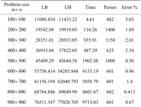
The results of our experiments are given in the following tables. The column “Passes” presented the number of time we go through the algorithm looking for bet- ter Lower bound and upper bound. The last row corre- sponds to the error percentage value which shows the percentage gap between the lower and the upper bound- where

UB LB Error%

UB

 

In Table 1, we use eight instances generated as in the

work of Barahona and Anbil [10], and the work of Cor- nuejols et al. [12].

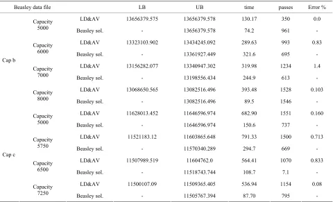
In Table 2, Beasly’s test problem has been considered

and solved using the method of this work. Comparing our solutions with Beasley’s, we notice that we were able to obtain a very close solution of Beasley’s where the reason is using different machines to get the solutions see (Beasley [13]). The gap between our solutions and Beasley’s is less than 1%.

10. Conclusion

[image:4.595.307.539.559.734.2]

A good lower bound has been achieved on the solution of the Capacitated Facility Location Problem considered in

Table 1. The results of solving different size of CFLB pro- blem using Lagrangean Relaxation Technique and Volume algorithm.

Problem size

m n LB UB Time Passes Error %

100 100 11088.854 11433.22 4.61 482 3.03

200 200 19542.08 19919.05 116.26 1400 1.89

300 300 28351.01 28933.05 935.91 1150 2.01

400 400 36935.04 37822.05 487.29 625 2.34

500 500 45409.29 45644.58 1902.88 1000 0.50

600 600 53756.414 54285.848 4133.19 601 0.96

700 700 61156.194 62048.793 5058.79 601 1.4

800 800 68764.846 69049.99 8601.67 602 0.413

900 900 76511.347 77028.705 9715.03 601 0.67

(5)

[image:5.595.59.539.101.392.2]

Table 2. Comparing the results obtain using Lagrangean Relaxation Technique and Volume algorithm with Beasley results.

Beasley data file LB UB time passes Error %

LD&AV 13656379.575 13656379.578 130.17 350 0.0 Capacity

5000 _{Beasley sol.} _- _13656379.578 _74.2 ₉₆₁ _-

LD&AV 13323103.902 13434245.092 289.63 993 0.83

Capacity

6000 _{Beasley sol.} _- _13361927.449 _321.6 ₆₉₅ _-

LD&AV 13156282.077 13340947.302 319.98 1234 1.4

Capacity

7000 _{Beasley sol.} _- _13198556.434 _244.9 ₆₁₃ _-

LD&AV 13068650.565 13082516.496 393.48 1528 0.103

Cap b

Capacity

8000 _{Beasley sol.} _- _13082516.496 _89.5 ₁₅₄₆ _-

LD&AV 11628013.452 11646596.974 682.90 1551 0.160

Capacity

5000 _{Beasley sol.} _- _11646596.974 _150.6 ₇₃₇ _-

LD&AV 11521183.12 11603865.648 791.33 1500 0.713

Capacity

5750 _{Beasley sol.} _- _11570340.289 _294.7 ₆₆₉ _-

LD&AV 11507989.519 11604762.0 564.41 1070 0.833

Capacity

6500 _{Beasley sol.} _- _11518743.744 _108.7 _7.1 _-

LD&AV 11500107.09 11509365.405 536.94 1154 0.08

Cap c

Capacity

7250 _{Beasley sol.} _- _11505767.394 _87.70 ₇₉₅ _-

this work. The Volume algorithm has been used to improve the lower bound.

REFERENCES

[1] K. Holmberg, M. Ronnqvist and D. Yuan, “An Exact Algorithm for the Capacitated Facility Location Problems with Single Sourcing,” European Journal of Operational Research, Vol. 113, No. 3, 1999, pp. 544-559.

doi:10.1016/S0377-2217(98)00008-3

[2] S. Melkote and M. S. Daskin, “Capacitated Facility Loca- tion-Network Design Problems,” European Journal of Operational Research, Vol. 129, No. 3, 2001, pp. 481- 495. doi:10.1016/S0377-2217(99)00464-6

[3] R. K. Ahuja, J. B. Orlin, S. Pallottino, M. P. Scaparra and M. G. Scutella, “A Multiexchange Heuristic for the Sin- gle-Source Capacitated Facility Location Problem,” Man- agement Science, Vol. 50, No. 6, 2004, pp. 749-760. doi:10.1287/mnsc.1030.0193

[4] M. J. Cortinhal and M. E. Captivo, “Genetic Algorithms for the Single Source Capacitated Location Problem,”

Metaheuristics: Computer Decision-Making, Vol. 86,

2004, pp. 187-216.

[5] I. A. Contreras and J. A. Diaz, “Scatter Search for the Single Source Capacitated Facility Location Problem,”

Annals of Operations Research, Vol. 157, No. 1, 2008, pp. 73-89. doi:10.1007/s10479-007-0193-1

[6] M. Leitner and G. R. Raidl, “A Lagrangian Decomposi- tion Based Heuristic for Capacitated Connected Facility

Location,” In: S. Voß and M. Caserta, Eds., Proceedings of the 8th Metaheuristic International Conference (MIC

2009), Hamburg, 13-16 July 2009.

[7] M. Held and R. M. Karp, “The Travelling Salesman Prob- lem and Minimum Spanning Trees,” Operations Re- search, Vol. 18, No. 6, 1970, pp. 1138-1162.

doi:10.1287/opre.18.6.1138

[8] E. J. Alenezy, “Practical Techniques to Solve Capacitated Facility Location Problem,” Far East Journal of Mathe- matical Sciences (FJMS), Vol. 37, No. 1, 2010, pp. 49-60.

[9] M. Held, C. Wolf and H. Crowder, “Validation Subgra-dient Optimisation,” Mathematical Programming, Vol. 6,

No. 1, 1974, pp. 62-88. doi:10.1007/BF01580223

[10] F. Barahona and R. Anbil, “The Volume Algorithm: Pro- ducing Primal Solutions Using a Subgradient Method,”

Mathematical Programming, Vol. 87, No. 3, 2000, pp.

385-399. doi:10.1007/s101070050002

[11] D. Serra, S. Ratick and C. Revelle, “The Maximum Cap- ture Problem with Uncertainty,” Environment and Plan- ning, Vol. B23, No. 1, 1996, pp. 49-59.

[12] G. Cornuejols, R. Sridharn and J. Thizy, “A Comparison of Heuristics and Relaxations for the Capacitated Plant Location Problem,” European Journal and Opertional Research, Vol. 50, No. 3, 1991, pp. 280-297.

doi:10.1016/0377-2217(91)90261-S