Computational Protein Interface Design and Prediction with Experimental Constraints
Steven Morgan Lewis
A dissertation submitted to the faculty of the University of North Carolina at Chapel Hill in partial fulfillment of the requirements for the degree of Doctor of Philosophy in the
Department of Biochemistry and Biophysics (Program in Molecular and Cellular Biophysics).
Chapel Hill 2012
Approved by:
Abstract
STEVEN LEWIS: Computational Protein Interface Design and Prediction with Experimental Constraints
(Under the direction of Brian Kuhlman)
Computational modeling is a powerful companion to direct experimental testing, because it allows researchers to answer questions that are too expensive to test in the lab or insurmountable with existing techniques. The development of algorithms and a computational framework in which to use them form an upfront cost of modeling. The Rosetta software suite is one such framework. Our recent rewrite of Rosetta using modular, reusable, object-oriented code allows Rosetta developers to rapidly and easily create modeling protocols to address new biological questions, reducing the investment needed to use computer modeling and enabling easier biologist-modeler collaborations.
We developed two other new Rosetta protocols, FloppyTail and
This...is proteins. Proteins compile.
Acknowledgements
This is the scariest part of this thesis to write. Forgetting to cite a paper or mislabeling a graph is fixable, but forgetting to thank someone is irreparable. As this thesis is really a story of collaborations, none of the interesting bits could have happened without the help of others.
I guess my advisor Brian Kuhlman comes first. My main project,
AnchoredDesign, is built around the core of a protocol idea he handed to me at the beginning of my work here. All of my side projects, which have led to many
publications, have come from him calling me into his office and pitching an idea to me. He quickly learned what sort of protocol development I'm good at and knows how to frame collaborations so that I can make my modeling contributions most efficiently. I'm very grateful!
The AnchoredDesign stories told in this thesis have help from several groups of people. The protocol development itself (this goes for the other protocols as well) received assistance from many members of the Rosetta community. We'll run out of ink if I name names, but generally anyone who's written a useful Mover has earned my thanks.
paper (Chapter 2). I had only the vaguest ideas of how to prove my protocol; the benchmarking we actually performed worked out great.
The SH3 domain story with AnchoredDesign (Chapter 3) is thanks to Akash Gulyani and Klaus Hahn, along with contributions from Brian Kay and his lab. I'm grateful to have my modeling supporting such an interesting biosensor story. Doug Renfrew was instrumental in getting Rosetta ready to handle Mero53, both indirectly with his own thesis work and directly in assisting with generation of parameter files and rotamer libraries.
The Keap1 AnchoredDesign story (Chapter 4) would have gotten nowhere
without a lot of help from other members of the Kuhlman lab. Gurkan Guntas performed most of the DNA work and a reasonable fraction of the protein work for that story, and Tom Lane did a big chunk of protein purification and several binding experiments as a rotation project. Pretty much every member of the lab contributed either minor reagents or experimental expertise at some point in the project.
The two ubiquitin stories (Chapters 5 and 6) were mostly due to the hard work of Gary Kleiger and Anjanabha Saha in Ray Deshaies's lab. Their willingness to cleverly design experiments that step around the limitations of Rosetta models really improved those papers. Doug Renfrew and Phil Bradley contributed ideas and code into making the thioester bond in Chapter 6 work.
allowed the originally-single-purpose code written for the ubiquitin chapters to live on in new projects and really proven to me that well written algorithms are eternal.
Many of UNC's administrative crew have been helpful to me over the years. Our department's administrative office is the friendliest and most helpful group of people I've ever met. The Research Computing folks, who administer the supercomputer clusters on which all the modeling results in this thesis were computed, have also been incredibly helpful in debugging cluster issues and letting me override my processor allotment in emergencies.
Table of Contents
List of Tables...xi
List of Figures...xii
Chapter 1...1
Rosetta...1
Rosetta’s tools...3
Tethered docking...6
AnchoredDesign...7
New interfaces created with AnchoredDesign...8
AnchoredDesign predicts qualities of monobody-SH3 interfaces...10
FloppyTail modeling of Cdc34-Cul1-Rbx1...11
UBQ_E2_thioester modeling of the ubiquitin-Cdc34 interface...13
Summary...15
References...18
Chapter 2...22
Introduction...22
Methods...26
Results...36
Discussion...42
Chapter 3...69
Introduction...69
Methods...72
Results...77
Conclusion...79
References...88
Chapter 4...90
Introduction...90
Methods...93
Results...102
Discussion...106
References...118
Chapter 5: ...122
Introduction...122
Methods...124
Results...128
Conclusions...129
References...139
Chapter 6...141
Introduction...141
Methods...143
Results...146
List of Tables
Table 2.1: Annotated scorefile headers...58
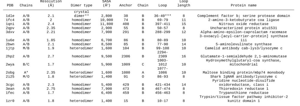
Table 2.2: Input structures and accessory data...59
Table 2.3: RMSD of lowest-scoring models...60
Table 2.4: Comparison of loop closure methods...61
Table 2.S1: AnchoredDesign scorefunction...62
Table 2.S2: Effects of anchor displacement...63
Table 4.1: Loop length and anchor placement constructs...114
Table 4.2: Contents of directed library...115
Table 4.3: Affinities of Keap1-binding monobodies by ITC and FP...116
List of Figures
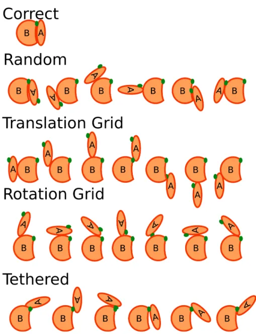
Figure 1.1: Search spaces for different docking methods...16
Figure 1.2: A flow diagram representing biology-modeling collaboration...17
Figure 2.1: Anchor insertion...46
Figure 2.2: AnchoredDesign treatment of rigid-body and loop degrees of freedom...47
Figure 2.3: Protocol flowchart...48
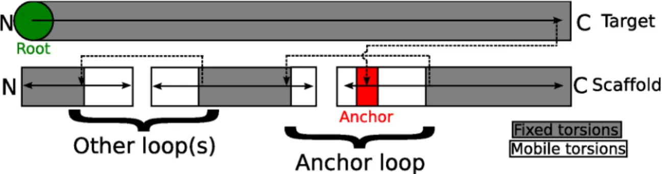
Figure 2.4: Fold tree diagram...49
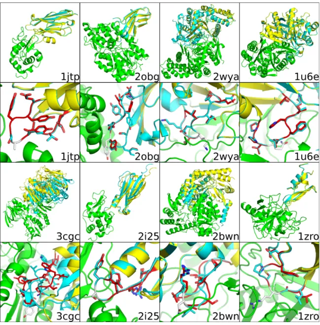
Figure 2.5: Best scoring prediction for 8 complexes...50
Figure 2.6: IRMSD versus score plots...51
Figure 2.7: Poorly predicted 1qni and 2hp2 loops...52
Figure 2.S1: Annotated AnchoredDesign results...53
Figure 2.S2: Best scoring prediction for 8 complexes...54
Figure 2.S3: LRMSD versus score plots...55
Figure 2.S4: Loop RMSD versus score plots...56
Figure 2.S5: 2obg and 1fc4 sampling...57
Figure 3.1: Src-family kinase autoinhibition...80
Figure 3.2: A fibronectin monobody bound to its target...81
Figure 3.3: Mero53 dye structure and chemical moieties...82
Figure 3.4: 1F11-SH3 complex model...83
Figure 3.5: 1F11-SH3 models for the 3 dye positions...84
Figure 3.6: Modeling of the 1F11 dye–SH3 interface...85
Figure 3.8: Modeling 1F11-SH3 functionalized at position 55...87
Figure 4.1: Keap1 has a positively charged binding pocket for DEETGE...109
Figure 4.2: Round 1 modeling options...110
Figure 4.3: Round 2 modeling options...111
Figure 4.4: Design models selected by phage display...112
Figure 4.5: Alanized positions in 5_2 and 8_1...113
Figure 5.1: The basic patch on Cul1...132
Figure 5.2: The Cdc34 tail's extended length and acidic residues...133
Figure 5.3: FloppyTail control flow...134
Figure 5.4: The top 20 Cdc34-Cul1-Rbx1 models by binding energy...135
Figure 5.5: A close-up view of the Cdc34 tail in the best-scoring model...136
Figure 5.6: Cdc34 C227-Cul1 K679 distance distribution by model score...137
Figure 5.7: FloppyTail in new systems...138
Figure 6.1: Disagreement about E2-ubiquitin interface models...150
Figure 6.2: Modeled torsions near the thioester bond...151
Figure 6.3: UBQ_E2_thioester protocol flow...152
Figure 6.4: A comparison of constrained and unconstrained models...153
Figure 6.5: Model interface suggests I44 interactions...154
Chapter 1 Introduction
Computational modeling of protein structure is a powerful tool for probing the mysteries of life at the smallest scale. Modeling allows us to develop, test, and discard hypotheses much more quickly than bench science. It also enables the testing of hypotheses that are either impossible or extremely challenging to address through conventional means. The ability to test many hypotheses simultaneously allows a researcher to focus expensive bench resources only on the hypotheses best supported by relatively inexpensive modeling data, making the research more efficient and economical. The extra power afforded by computational modeling requires an upfront investment needed to create the modeling tools and verify them against problems with known answers. These costs can be ameliorated by adjustments to the process by which modeling tools are generated. This thesis demonstrates how advances in the Rosetta protein modeling framework created an environment in which new modeling techniques can be rapidly developed, reducing this first investment cost for new techniques in computational modeling.
Rosetta
Rosetta is a large suite of programs supported by dozens of developers at a
and homology modeling [1, 2]. Rosetta’s successes are numerous, including the first design of a novel protein fold [3] and good showings in protein structure prediction [4] and protein-protein docking prediction [5] competitions.
Early versions of Rosetta were written in FORTRAN77, which was machine-translated into C++ and released as Rosetta++ [6]. The haphazard development of the Rosetta++ codebase greatly complicated generation and dissemination of new protocols written as part of the Rosetta++ suite. In particular, adding new protocols to Rosetta often required adding a few lines of code in the middle of many other existing bits of code, instead of developing new modules as single units. The Rosetta community therefore decided to rewrite the whole body of code, with the major part of the rewrite commencing in 2007. We released this rewritten Rosetta as the Rosetta3 applications suite.
focus on optimizing search and scoring functions at a high level without having to re-implement ideas at every level of minutiae in the whole program.
This thesis will describe the development, purpose, and results of three different executables that have been released as part of the Rosetta3 suite. In each case, the programming flexibility granted by Rosetta3's refactoring was essential to their success. For the AnchoredDesign suite, Rosetta3’s modularity allowed the development of a very complicated protocol for the complex problem of flexible protein-protein interface design, which was built with simple calls to Rosetta’s packing, minimization, and loop modeling routines [7]. For the FloppyTail and UBQ_E2_thioester protocols, Rosetta’s flexibility allowed rapid development of modeling protocols designed to answer a specific biologic question in collaboration with biologists [8, 9].
Rosetta’s tools
Protein modeling algorithms are built on two underlying techniques: a scoring function which determines the thermodynamic plausibility of a structure, and a search function which proposes structures for scoring. This thesis is focused on the
development of algorithms with novel search techniques, so it relies on Rosetta's previously published and proven scoring functions [3, 10].
accepted, which drives the trajectory to ever-improving scores and structures. If the score gets worse, the changes are accepted with a probability inversely related to the size of the score change (the Metropolis criterion) [11]. This occasional increase in score allows escape from local energy minima during the search for the global energy minimum. Metropolis-Monte Carlo does not guarantee finding global energy minima, but has proven to be a fast method for finding plausible protein structures [3].
The new protocols developed in this thesis use Rosetta's score function and use Monte Carlo as a base for their search functions. Monte Carlo alone does not specify how random modifications are selected, just how the modifications accumulate. The novelty of the protein modeling algorithms in this thesis lies in what random
modifications are proposed during Monte Carlo modeling, and how those modifications are implemented.
Each individual modification to a protein structure samples some degree of freedom in the model. Rosetta uses internal coordinates to place atoms in an AtomTree, also known as an Internal Coordinates Model (ICM) [6, 12]. This
The complexity of an atomic level AtomTree is often softened by use of a residue-level FoldTree [13]. The FoldTree operates on the same principles by organizing an underlying AtomTree, but allows the programmer to consider whole residue units instead of individual atoms. This FoldTree is very flexible in that it allows the development of many sorts of modeling approaches in Rosetta [13].
A key effect of the internal coordinate representation of proteins is the cascading effect of degree of freedom movement caused by the dependence of atoms late in the chain on those early in the chain. The three-dimensional spatial coordinates for any atom are recalculated from the positions of the atoms it depends on, and the internal coordinate degrees of freedom connecting the atoms. This means that a rotation of one backbone torsion will propagate from parent to child atoms, ultimately causing all downstream dependent atoms to move as well. For some modeling problems, this is a downside of the ICM approach, but for the approaches detailed in this thesis it is critically useful.
Another part of the Rosetta3 rewrite that is important for understanding this thesis is the centrality of the Mover idea. In Rosetta, a Mover is a C++ class which takes a protein conformation, alters it in some fashion, and returns a new protein conformation [6]. Movers therefore plug into a Monte Carlo search protocol by proposing
protocols, and the innermost represent Rosetta's published algorithms for packing, minimization, and structure manipulation.
Tethered docking
Each of the new Rosetta protocols presented here treats a problem in protein-protein interface prediction and docking, with the twist that in each case some wrinkle in the modeling precludes the use of standard rigid-body docking protocols. For every protocol, there is some rigid constraint tethering together the proteins being modeled— either a covalent connection between proteins (UBQ_E2_thioester) or a partially known interface to be maintained (AnchoredDesign and FloppyTail). It should be noted that the applications were not developed with the intention of treating similar problems; rather, each was developed in response to a particular modeling or biological problem of interest. The Rosetta application developed to address each of these problems is unique in that it only searches through solutions that meet the tethering constraint—unproductive conformations that would be rejected for failing the constraint are never searched.
models that never satisfied the preexisting constraints. These sorts of search functions deal with constraints by filtering or ranking on the constraint post hoc. Figure 1.1 demonstrates how these sorts of docking search protocols propose models for scoring.
For the tethered docking problems addressed in this thesis, the tethering constraint demands that some portion of the interface remain intact. Instead of freely varying the rigid-body degree of freedom between proteins, this tether connection can be remodeled to produce candidate docked structures. Flexing the point of contact between the two rigid bodies produces motion that mimics rigid-body docking. To produce this effect, the folding pathway (AtomTree) through which Rosetta converts internal coordinates to three-dimensional coordinates passes through this tether region between the upstream and downstream proteins. This means that modifications to the tether affect all atoms
downstream in the folding pathway, allowing the moving side of the interface to swing through space as the tether is sampled. All of the Rosetta modules presented in this thesis take advantage of this tethered atom tree structure to substitute tether remodeling for rigid-body docking, allowing sampling to focus tightly on conformations that respect the tether constraint. Figure 1.1 demonstrates how the Rosetta tethered docking applications in this thesis propose models for scoring in a fashion consistent with the tethering
constraint.
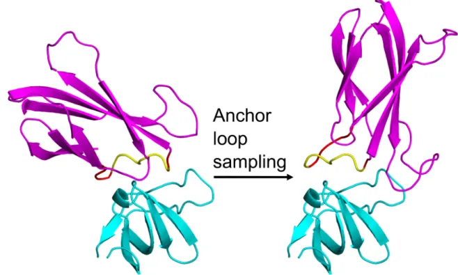
AnchoredDesign
The first Rosetta3 application developed during the course of this thesis,
new interface between the target and a desired scaffold. This graft, called the anchor, is inserted into a scaffold loop and held rigidly affixed to the target while the scaffold is sampled around it, as demonstrated by Figure 2.1. The purpose of this anchoring is twofold: first, it may allow for some small baseline affinity between the design scaffold and the target, and second, it ensures that the scaffold redesign is aimed at an interface-compatible region of the target surface. Protein surfaces that form transient protein-protein interfaces tend to have more aromatic and fewer charged residues [20], suggesting that targeting preexisting binding interfaces will make it easier to design binding partners.
The algorithm uses both loop modeling and design iteratively to produce flexible backbone interface design. The grafted anchor, in a loop of the design scaffold
contacting the target, serves as the docking tether. Docking degrees of freedom are sampled by modifying the loop containing the anchor, which results in a swinging motion about the interface and ultimately altered rigid-body orientation, as demonstrated by Figure 2.2. Other surface loops of the scaffold can also be sampled using Rosetta's implementation of the Cyclic Coordinate Descent [21] or kinematic loop closure [22] algorithms, ensuring good loop-mediated shape complementarity between the target and design scaffold. Rosetta's proven design techniques [3] are used to sample sequence space of the moving loops to select sequence that will best fold into the desired structure. Computational benchmarking of this algorithm demonstrated its utility [7].
New interfaces created with AnchoredDesign
β-propeller domain [24]. As reported in Chapter 4, these designed monobodies bind with affinities resembling the wild-type partners of Keap1, and partial designs enhanced with phage display techniques bind much tighter than known partners for Keap1.
Our design scaffold, human fibronectin, domain type 3, repeat 10 (10FNIII), is well known as an adaptable scaffold for generating new protein-protein interfaces [23, 25-27]. Figure 3.2 demonstrates such an interface. The AnchoredDesign protocol was developed with this scaffold in mind: the algorithm designs flexible loops at the surface of the scaffold, and 10FNIII has two surface loops (labeled FG and BC, after the beta strands they occur between) that are very amenable to mutation [23]. Insertion of the anchor in either loop allows AnchoredDesign to use that loop as a flexing point for tethered docking, while remodeling and redesigning both loops to generate a new protein-protein interface. Several crystal structures of 10FNIII are available, including both wild type fibronectin [28, 29] and derived monobodies in complex with partners [27].
Keap1 is an interesting target due to the structure of its naturally-occurring protein-protein interface. It natively binds a short hairpin structure from its partner Nrf2, as revealed in a 1.5 Å resolution crystal structure [24] seen in Figure 4.1. This hairpin has geometrically close end points, which makes it ideal for insertion into a fibronectin loop as an anchor.
target, but experiments designed to elucidate the structure of the monobody/Keap1 complexes have produced either no or ambiguous results.
The success of AnchoredDesign at generating sequences which bind their intended targets showcases how Rosetta3's restructuring makes modeling simpler. The protocol addresses one of the most complex current topics in protein modeling: flexible, one-sided protein-protein interface design. An algorithm for the problem must handle searching through rigid-body, backbone, and sequence space. All of this complexity is manageable due to the ease of use of Rosetta's many modular tools for protein modeling.
AnchoredDesign predicts qualities of monobody-SH3 interfaces
AnchoredDesign has also been proven capable of predicting some qualities of an engineered fluorophore-labeled biosensor [30], reported in Chapter 3. We were interested in generating reagents that used fluorescence to signal the location and activity of SH3 (Src Homology 3) domains. We used an existing fibronectin-based monobody affinity reagent, 1F11, which had been evolved to bind the cSrc SH3 domain [26]. Fluorophores chemically conjugated to different positions on the monobody were found to vary in their response to monobody-cSrc binding. Specifically, at some scaffold positions, the
fluorphore's intensity changed on cSrc binding, but at other positions, it did not.
fluorophore. This fluorophore could then be dropped into Rosetta modeling with no modifications to the central packing, minimization, or loop closure algorithms, and only minor modifications to AnchoredDesign itself. Ultimately, AnchoredDesign was able to discriminate positions that showed a fluorescence intensity change on binding from those that did not by showing a change in solvent-accessible surface area of the polar groups of the fluorophore between the bound and unbound states [30].
This biosensor modeling project exemplifies the power of computational
modeling as a companion to biology, and demonstrates how Rosetta3's structure reduces the upfront investment needed to get modeling data. Here, an application written to perform protein-protein interface design was rapidly adapted for fixed-sequence modeling of a known interface, including the chemically conjugated fluorophore. The modularity of the non-canonical amino acid protocols in Rosetta allowed easy drop-in of the novel fluorophore into an existing protocol. This sort of biology-modeling feedback is a major benefit of the structural improvements in Rosetta 3. Figure 1.2 presents a flowchart model of how these sorts of biology-modeling collaborations function.
FloppyTail modeling of Cdc34-Cul1-Rbx1
FloppyTail [8] was originally developed in collaboration with a biology-focused lab led by Raymond J. Deshaies in order to answer a specific question about a protein complex of interest. The binding of two proteins, ubiquitin E3 ligase complex SCF (Skp, Cullin, F-box) and Cdc34, was known to be affected by the presence of a long, highly negatively charged C-terminal tail on Cdc34. Sequence homology to solved structures implied that Cdc34 bound SCF via the RING domain in the Rbx1 subunit of SCF, but there were no structures of the complex, nor any Cdc34 structures containing the tail. Experiments demonstrated that the charged tail was necessary for the normal biologic function of these proteins [32]. The SCF complex contains a highly positively charged cleft or patch in its Cul1 subunit (Figure 5.1), and mutations in this region cause defects in ubiquitin transfer [8]. These data lead to the hypothesis that the acidic tail and basic cleft may interacting as a second binding site between SCF and Cdc34.
No Rosetta application that existed at the time was capable of handling this sort of question. However, Rosetta3's modular structure allowed the rapid development of the FloppyTail application to fit the purpose, detailed in Figure 5.3. Search algorithm tools originally written for ab initio structure prediction and loop modeling were combined to allow sampling of the volume available to the flexible tail, even though it does not have significant secondary structure as ab initio requires, nor is it a closed loop as loop modeling assumes. FloppyTail keeps the flexible region being modeled tethered to the appropriate attachment points on preexisting structures of the other domains in the system, and modifies backbone and sidechain torsions in the flexible region to determine where and how they might associate. This tethering limits the search space for the interface between the Cdc34 tail and SCF to regions within geometric reach of the tail without breaking its tether connection to Cdc34.
This modeling protocol allowed prediction of certain features of the putative tail-cleft interface which were confirmed by experiment [8]. Specifically, the models were used to predict that Cul1 residue K679 and Cdc34 residue C227 were nearby in the bound state, which was demonstrated by chemical crosslinking. This completes the biology-modeling collaboration in Figure 1.2: the Deshaies lab posed a structural question, a Rosetta protocol was developed to address the question, and the resulting models were used to make verifiable predictions about the interface which deepened understanding of the biology of the system.
UBQ_E2_thioester modeling of the ubiquitin-Cdc34 interface
This time, the nature of the interface between the E2 Cdc34 and ubiquitin was of interest. As with the SCF/E2 tail interface in the FloppyTail project, no structure of the interface existed, but experiments generated data constraining what the interface might look like. Modeling of this interface is discussed in Chapter 6.
The Cdc34-ubiquitin interface is not a normal, labile protein-protein interface. It is instead dominated by the thioester bond that forms between ubiquitin's C-terminus and the catalytic cysteine residue of Cdc34 [9], shown in Figure 6.2. This thioester bond is normal for a ubiquitin-charged E2 that is ferrying activated ubiquitin to an E3 [38], but thioester bonds are rare in proteins in general. While this bond is sufficiently
thermodynamically unstable to make structural studies challenging [9, 39], it is a covalent bond, so candidate interface structures must take it into account.
The existence of the thioester bond makes this modeling problem another example of a tethered docking experiment. The most interesting degree of freedom in the system is the rigid-body orientation between ubiquitin and Cdc34. While the possible solution space is enormously limited by the existence of this covalent bond, it is still essentially a docking problem regarding a non-obligate interface.
Besides the thioester bond, mutational data at the interface [9], along with a model structure of a different E2-ubiquitin interface [39], were available for guiding the
modeling of the Cdc34-ubiquitin interface. To model the interface between ubiquitin and Cdc34, including specific treatment of the embedded thioester bond, the
sample the backbone for the ubiquitin C-terminal tail conjugated to Cdc34 and determine what envelope on the surface of Cdc34 it could occupy, as well as identify possible binding modes. This treatment of the tethered docking problem satisfies the covalent thioester constraint by including it in the modeling from the beginning and searching for solutions pivoting around the thioester, instead of performing general docking and filtering for thioester-compatible solutions.
These models were used to predict a rescue mutation, Cdc34 S129L, for a known mutation that disrupted the Cdc34-ubiquitin interface, ubiquitin I44A. The success of this rescue mutation reiterates the power of rapid, collaborative program development in Rosetta3. As with FloppyTail, a biological question was addressed by the development of a specific Rosetta application. Again, the modeling results were verified by
experiment in the biological system of interest.
Summary
Figure 1.1: Search spaces for different docking methods
This figure demonstrates how different docking search methods propose models for scoring. The correct model for the A and B complex is shown at the top. Note the shape complementarity and the coalignment of the green dot, which represents an
Figure 1.2: A flow diagram representing biology-modeling collaboration
References
1. Kaufmann KW, Lemmon GH, Deluca SL, Sheehan JH, Meiler J. (2010)
Practically useful: What the rosetta protein modeling suite can do for you. Biochemistry 49(14): 2987-2998. 10.1021/bi902153g.
2. Das R, Baker D. (2008) Macromolecular modeling with rosetta. Annu Rev Biochem 77: 363-382. 10.1146/annurev.biochem.77.062906.171838.
3. Kuhlman B, Dantas G, Ireton GC, Varani G, Stoddard BL, et al. (2003) Design of a novel globular protein fold with atomic-level accuracy. Science 302(5649): 1364-1368. 4. Raman S, Vernon R, Thompson J, Tyka M, Sadreyev R, et al. (2009) Structure prediction for CASP8 with all-atom refinement using rosetta. Proteins 77 Suppl 9: 89-99. 10.1002/prot.22540.
5. Fleishman SJ, Corn JE, Strauch EM, Whitehead TA, Andre I, et al. (2010) Rosetta in CAPRI rounds 13-19. Proteins 78(15): 3212-3218. 10.1002/prot.22784.
6. Leaver-Fay A, Tyka M, Lewis SM, Lange OF, Thompson J, et al. (2011) ROSETTA3: An object-oriented software suite for the simulation and design of
macromolecules. Methods Enzymol 487: 545-574. 10.1016/B978-0-12-381270-4.00019-6.
7. Lewis SM, Kuhlman BA. (2011) Anchored design of protein-protein interfaces. PLoS One 6(6): e20872. 10.1371/journal.pone.0020872.
8. Kleiger G, Saha A, Lewis S, Kuhlman B, Deshaies RJ. (2009) Rapid E2-E3 assembly and disassembly enable processive ubiquitylation of cullin-RING ubiquitin ligase substrates. Cell 139(5): 957-968. 10.1016/j.cell.2009.10.030.
9. Saha A, Lewis S, Kleiger G, Kuhlman B, Deshaies RJ. (2011) Essential role for ubiquitin-ubiquitin-conjugating enzyme interaction in ubiquitin discharge from Cdc34 to substrate. Mol Cell 42(1): 75-83. 10.1016/j.molcel.2011.03.016.
10. Rohl CA, Strauss CEM, Misura KMS, Baker D. (2004) Protein structure prediction using rosetta. Methods Enzymol 383: 66-+.
11. Metropolis N, Rosenbluth AW, Rosenbluth MN, Teller AH, Teller E. (1953) Equation of state calculations by fast computing machines. J Chem Phys 21(6): 1087-1092.
13. Wang C, Bradley P, Baker D. (2007) Protein-protein docking with backbone flexibility. J Mol Biol 373(2): 503-519.
14. Gray JJ, Moughon S, Wang C, Schueler-Furman O, Kuhlman B, et al. (2003) Protein-protein docking with simultaneous optimization of rigid-body displacement and side-chain conformations. J Mol Biol 331(1): 281-299.
15. Chaudhury S, Berrondo M, Weitzner BD, Muthu P, Bergman H, et al. (2011) Benchmarking and analysis of protein docking performance in rosetta v3.2. PLoS One 6(8): e22477. 10.1371/journal.pone.0022477.
16. Dominguez C, Boelens R, Bonvin AM. (2003) HADDOCK: A protein-protein docking approach based on biochemical or biophysical information. J Am Chem Soc 125(7): 1731-1737. 10.1021/ja026939x.
17. Chen R, Weng Z. (2002) Docking unbound proteins using shape complementarity, desolvation, and electrostatics. Proteins: Structure, Function, and Bioinformatics 47(3): 281-294. 10.1002/prot.10092.
18. Chen R, Li L, Weng Z. (2003) ZDOCK: An initial-stage protein-docking algorithm. Proteins 52(1): 80-87. 10.1002/prot.10389.
19. Comeau SR, Gatchell DW, Vajda S, Camacho CJ. (2004) ClusPro: An automated docking and discrimination method for the prediction of protein complexes.
Bioinformatics 20(1): 45-50.
20. Lo Conte L, Chothia C, Janin J. (1999) The atomic structure of protein-protein recognition sites. J Mol Biol 285(5): 2177-2198.
21. Canutescu AA, Dunbrack RL. (2003) Cyclic coordinate descent: A robotics algorithm for protein loop closure. Protein Sci 12(5): 963-972.
22. Mandell DJ, Coutsias EA, Kortemme T. (2009) Sub-angstrom accuracy in protein loop reconstruction by robotics-inspired conformational sampling. Nature Methods 6(8): 551-552. 10.1038/nmeth0809-551.
23. Koide A, Bailey CW, Huang XL, Koide S. (1998) The fibronectin type III domain as a scaffold for novel binding proteins. J Mol Biol 284(4): 1141-1151.
24. Lo SC, Li X, Henzl MT, Beamer LJ, Hannink M. (2006) Structure of the
25. Koide A, Abbatiello S, Rothgery L, Koide S. (2002) Probing protein
conformational changes in living cells by using designer binding proteins: Application to the estrogen receptor. Proc Natl Acad Sci U S A 99(3): 1253-1258.
26. Karatan E, Merguerian M, Han Z, Scholle MD, Koide S, et al. (2004) Molecular recognition properties of FN3 monobodies that bind the src SH3 domain. Chem Biol 11(6): 835-844. 10.1016/j.chembiol.2004.04.009.
27. Koide A, Gilbreth RN, Esaki K, Tereshko V, Koide S. (2007) High-affinity single-domain binding proteins with a binary-code interface. Proc Natl Acad Sci U S A 104(16): 6632-6637.
28. Dickinson CD, Veerapandian B, Dai XP, Hamlin RC, Xuong NH, et al. (1994) Crystal-structure of the 10th type-iii cell-adhesion module of human fibronectin. J Mol Biol 236(4): 1079-1092.
29. Leahy DJ, Aukhil I, Erickson HP. (1996) 2.0 angstrom crystal structure of a four-domain segment of human fibronectin encompassing the RGD loop and synergy region. Cell 84(1): 155-164.
30. Gulyani A, Vitriol E, Allen R, Wu J, Gremyachinskiy D, et al. (2011) A biosensor generated via high-throughput screening quantifies cell edge src dynamics. Nat Chem Biol 7(7): 437-444. 10.1038/nchembio.585; 10.1038/nchembio.585.
31. Renfrew PD, Choi EJ, Bonneau R, Kuhlman B,. (2012) Incorporation of
noncanonical amino acids into rosetta and use in computational protein-peptide interface design. PLoS ONE 7(3): e32637. Available:
http://dx.doi.org/10.1371%2Fjournal.pone.0032637 via the Internet.
32. Mathias N, Steussy CN, Goebl MG. (1998) An essential domain within Cdc34p is required for binding to a complex containing Cdc4p and Cdc53p in saccharomyces cerevisiae. J Biol Chem 273(7): 4040-4045.
33. Ceccarelli DF, Tang X, Pelletier B, Orlicky S, Xie W, et al. (2011) An allosteric inhibitor of the human Cdc34 ubiquitin-conjugating enzyme. Cell 145(7): 1075-1087. 10.1016/j.cell.2011.05.039.
34. Zheng N, Schulman BA, Song L, Miller JJ, Jeffrey PD, et al. (2002) Structure of the Cul1-Rbx1-Skp1-F boxSkp2 SCF ubiquitin ligase complex. Nature 416(6882): 703-709. 10.1038/416703a.
36. Ptak C, Prendergast JA, Hodgins R, Kay CM, Chau V, et al. (1994) Functional and physical characterization of the cell cycle ubiquitin-conjugating enzyme CDC34 (UBC3). identification of a functional determinant within the tail that facilitates CDC34 self-association. J Biol Chem 269(42): 26539-26545.
37. Cole C, Barber JD, Barton GJ. (2008) The jpred 3 secondary structure prediction server. Nucleic Acids Research 36(suppl 2): W197-W201. 10.1093/nar/gkn238.
38. Nandi D, Tahiliani P, Kumar A, Chandu D. (2006) The ubiquitin-proteasome system. J Biosci 31(1): 137-155.
Chapter 2
Anchored Design of Protein-Protein Interfaces
Introduction
Because so many human diseases are caused by dysregulation of proteins or protein-protein interactions, the need to experimentally or therapeutically adjust these systems is great. A powerful tool for probing protein networks is other proteins
engineered to bind particular naturally-occurring target proteins and modify or illuminate their behavior. To that end, many authors have introduced computational methods for creating these tool proteins, including both de novo binding partners and redesigns of existing interfaces.[1] One modeling suite used for this purpose, and many others, is Rosetta.[2]
Placing past successes in context, it remains quite challenging to create binding partners with desired functionality, and even minor successes are not routine.[3, 4] This is because interface design combines all the challenges of protein design, itself an incompletely solved problem, with the additional complication of docking orientation between the two proteins.
optimizations necessary to efficiently sample conformations and sequences preclude sampling both simultaneously. Recent flexible-backbone design methods modifying protein interfaces or loops include methods using local backbone minimization [6] and fragment insertion plus loop closure and design.[7, 8]
A second decision must be made when designing new interfaces: which proteins should interact? The two major methods for protein interface design include de novo
design, which creates an interface between previously non-interacting proteins, and interface redesign, which modifies the properties of existing interactors or homologs thereof. De novo designs offer the opportunity to engineer new functions into the interaction, at the great cost of having to create the interface from scratch.[6, 9, 10] Redesigns offer the opposite tradeoff: there is an interaction in place to start from, but the designs are restricted to modifying existing functions by increasing affinity [11-15] or altering specificities [16-18].
Here we propose a new method offering a blend of these strengths which we call AnchoredDesign. The method has been implemented as a protocol in the Rosetta3 software suite.[19] The method creates an interface between an arbitrary (and arbitrarily functional) scaffold and a target, but it also creates the interface along a known
interacting surface of the target, using information from a preexisting binding partner. The method accounts for backbone flexibility at the interface by iterating between loop remodeling and design.
characteristics. For example, the fibronectin domain type 3 repeat 10 (10FNIII or FN3) scaffold used by many researchers is an appropriate design scaffold.[20-25]
The first step of this new method is to create a nascent interface between the target and the scaffold, as described in Figure 2.1. A small sequence-contiguous portion of the target’s known partner is extracted, and its sequence identity and coordinates are inserted into a surface loop on the scaffold. This becomes the anchor. Standard Rosetta loop closure techniques can be used to close the scaffold’s modified loop.[26] This results in an intermediate structure containing the target, the scaffold, and a small
interface between them where the scaffold mimics the original binding partner. It is ripe for flexible redesign to create a real interface between the partners. Note that the use of this anchor guarantees that the new designed binder will bind to a surface area of the target overlapping the original partner’s area. This helps control the activity of the new binder by ensuring that experimenters know where it is binding. It also controls for the residue composition of the target surface as suggested by Lo Conte et al.[27]
After creating a nascent interface via grafting, the next step is flexible redesign. Normally one considers the docking problem when thinking about designing protein-protein interfaces. Here, the anchor precludes the use of whole-protein-protein rigid-body motion as in docking, because this would cause the loss of the anchor. Instead, loop remodeling of the loop containing the anchor is used to sample the rigid body space between the proteins, as in Figure 2.2. Holding the anchor in its original binding conformation, rigidly affixed to the target, and remodeling its loop will result in rigid-body
transformations between the target and scaffold. This allows us to use loop modeling to generate backbone flexibility at the interface and simultaneously sample possible binding modes of the scaffold. Other surface loops on the scaffold can be concurrently sampled to produce further surface complementarity.
For computational methods like these, benchmarking tests both help develop the protocol and demonstrate its utility. For the AnchoredDesign protocol, we have
assembled a set of 16 protein structures from the PDB. These structures were chosen on the basis of having an interfacial loop with an appropriate residue to serve as an anchor. The protocol can then be tested against these structures by deleting the conformation of the anchor-containing loop and using the protocol to predict the proper binding
orientation of the two proteins. This serves as a test of the loop modeling and interface predictions of the protocol. Here we present the protocol itself, as used for design or in these benchmarks, and the results of these fixed-sequence structure prediction
Methods
AnchoredDesign protocol
The AnchoredDesign protocol is written as an application in the Rosetta3
software suite, and first released with the 3.3 release. It was designed from the ground up within the Rosetta3 framework and thus takes advantage of all the modularity and ease-of-use offered by that foundation.[19] The protocol uses a multistage Metropolis Monte Carlo search protocol, with large perturbational movements in a reduced centroid
representation and smaller refining changes in a higher-resolution fully atomic phase. This sort of multistage centroid/fullatom protocol is common for Rosetta protocols.[26, 31, 32] Conceptually, the centroid phase is meant to sample conformational space widely and jump over relatively high energy barriers between conformations, whereas the
fullatom phase is meant to minimize a centroid candidate structure into its local energy minimum. To accomplish this, the protocol iteratively samples loop conformations and sidechain conformations, with interspersed opportunities for design. Figure 2.3 offers a diagram of program flow summarizing the major steps of the protocol.
account for the anchor; see details below. No sidechain optimization is necessary during centroid-mode perturbation, so after loop closure the algorithm proceeds directly into gradient minimization.[31] Backbone torsions at flexible loop positions are minimized to ensure good loop conformations and to perfect loop closure in the CCD case.
The second phase of the protocol is the refinement phase, which uses a fully atomic representation of the proteins. The use of a fullatom scorefunction, along with smaller-scale changes tested by Monte Carlo, allows this phase to refine the candidate structure produced in the perturbation phase. Here, CCD and KIC loop remodeling are also both available, although the CCD steps are softened to suggest smaller protein changes (described below). After each loop closure step, a quick fixed-sequence rotamer relaxation is performed [36], followed by a gradient minimization. The design portion of AnchoredDesign is incorporated during the fullatom phase by performing a sequence design and/or rotamer repacking on the interface region at user-defined intervals between loop remodeling cycles. Note that to reduce time spent repacking, all rotamer
rearrangements used in AnchoredDesign feature automatic detection of the relevant residues: loop residues, their neighbors, and interface residues are automatically included, whereas residues outside those regions (the protein cores and distal surfaces) are not modified during repacking.
Loop modeling for AnchoredDesign
selects new values for non-pivot torsions.[34] The modifications used here allow for the anchor positions to be excluded from the list of allowable pivots and modifiable non-pivot torsions; they do not otherwise affect the underlying algorithm at all.
CCD loop closure has also been slightly modified to account for the anchor. Normally, CCD closes a broken loop by iteratively altering phi and psi angles to attempt to bring the broken loop ends together.[33] Here, the anchor's torsions are held fixed during CCD; it has no effect on the algorithm other than introducing inflexible regions which act as a particularly long bond.
Rosetta loop sampling with CCD is normally paired with a perturbation step which breaks the loop and introduces diversity.[26] Here, multiple methods are offered for perturbation before CCD closure. In the perturbation phase, the simplest method offered is randomization of the phi/psi angles (within Ramachandran constraints) of several residues in the loop. Other options include several varieties of fragment-based [31] perturbation: pregenerated fragment sets, automatically generated sequence-specific fragment sets, or automatically generated sequence-nonspecific fragment sets are
allowed. The former options are more useful for structure prediction; the latter for design (where the final sequence is not known during the perturbation phase, so fragments of varying sequence are appropriate). In the refinement phase, large loop rearrangements are not desired, so only randomization of phi/psi angles, within a few degrees and Ramachandran constraints, is offered as a method of generating variation before CCD. Fragment insertion is not performed during the fullatom refinement.
modifying the anchor or core of either protein. Figure 2.4 is a Rosetta fold tree diagram representing an AnchoredDesign fold tree, modeled after those in Wang et al.[26] Rosetta regularly updates atomic coordinates from internal coordinates (bond lengths, angles, and torsions) held by the atom tree and fold tree data structures.[19] The group of atoms moved by the rotation of any one bond is controlled by the connectivity of the atom tree, which is in turn set by the more general fold tree. In AnchoredDesign, the fold tree is built in such a way that the anchor residues are dependent only on the target
protein, the anchor's loop depends on the anchor, and the scaffold (which is rigid around the loop) is dependent on the loop. This setup ensures that conformational changes to the anchor loop result in relative motion of the two proteins' cores: rigid-body sampling. Other surface loops are treated with a standard loop fold tree as in Wang et al.[26] Methods for target selection
Because appropriate interfaces for testing the AnchoredDesign approach are only a small fraction of the available interfaces in the PDB, an automated method was created to find interfaces with loops resembling an anchored loop. This method has been
released alongside AnchoredDesign as AnchorFinder within the 3.3 release. The AnchorFinder algorithm was written to help find appropriate benchmarking structures, but it can also suggest useful anchors against targets of biological interest.
a listing of the DSSP assignment and cross-interface neighbors for each residue in each structure studied, plus summaries for contiguous regions that meet user-specified thresholds for length, secondary structure, and number of cross-interface neighbors. Regions with many cross-interface neighbors represent candidate anchors. When using AnchoredDesign to create new interfaces, AnchorFinder can help identify plausible anchors, but for small numbers candidate target/partner structures, manual examination is sufficient.
To choose our benchmarking set, the highest-ranking results from AnchorFinder were examined individually. AnchorFinder was run against the entire PDB (snapshot May 2009). The top several hundred structures returned by AnchorFinder were filtered to ensure that the hits were biological dimers and had identifiable anchors. The
remaining hits contained redundant copies of many biological interactions due to multiple structures of some interactions, and multiple copies of one interaction within an
asymmetric unit. Single representatives of each biological interaction were chosen. In general benchmarking systems were chosen to have a variety of biological sources, structures, and functions. One benchmarking structure, 2obg [24], was chosen for its identity as a fibronectin monobody structure without it appearing in the top fraction of AnchorFinder results: it represents the sort of structure AnchoredDesign is intended to create.
Choosing anchors, loops, and designable positions
either buried large amounts of surface area across the interface or choosing a residue with a cross-interface hydrogen bond. For the purposes of this benchmarking, only single-residue anchors were allowed, although the algorithm is compatible with longer contiguous anchors.
For the design case, anchors will be grafted into a different protein. It is therefore important to choose an anchor with some internal structure and/or a very well-defined interaction with the protein partner; examples might be 4 residues of a hairpin turn binding into a cleft or a phosphotyrosine binding an SH2 domain, respectively. Another possibility is the use of hot-spot residues [38, 39], including those determined by fast computational tools [40, 41]. Ultimately, anchor choice is a dimension of conformational space that must be searched by testing different anchors. Anchors can be evaluated computationally by examining the scores assigned by Rosetta to models using different anchors.
For the benchmarking presented here, the length for the remodeled loop
containing the anchor was chosen by simply accumulating residues out from the anchor in both directions until non-loop secondary structure was encountered. Only this single loop was varied, although the code is compatible with multiple (non-anchored) surface loops on both sides of the interface.
loops should be must be determined manually by feeding different inputs to AnchoredDesign and comparing the quality of the resulting models.
Similarly, the choice of designable positions is dependent on knowledge of the scaffold. Scaffolds are presumably chosen on the basis of experimental experience with their tolerance to mutation (for example, fibronectin monobodies [22] or diverse other scaffolds [25]). The protocol assumes, but does not require, that the designable positions are all on flexible loops on one side of the interface (one-sided design). It will
nevertheless accept two-sided design problems or non-loop design positions. Designable positions that are near neither flexible loops nor the interface may fail to be designed as desired, because the protocol automatically freezes those portions of the protein.
Creating starting structures
For the benchmarking in this paper, inputs for AnchoredDesign were generated from the crystal structure interaction with little modification. Nonprotein atoms (waters, cryoprotectants, and in some cases ligands) were deleted. These were passed through a simple structure minimizer to relax out any clashes with the Rosetta scorefunction. This protocol, InterfaceStructMaker (Peter Benjamin Stranges, unpublished protocol)
performs a full-protein minimization and packing. It was determined that this
preparatory step had no effect on the RMSD of the best scoring models (data not shown); its purpose was to remove data artifacts due to clashes in the crystal structures. These minimized structures were then fed directly to AnchoredDesign. AnchoredDesign
In the design case, preparation of AnchoredDesign starting structures is much more complicated, because the anchor must be grafted from one structure into another. AnchoredDesign has a companion protocol also released with Rosetta3.3,
AnchoredPDBCreator, designed to take care of this process. Two structures embodying three protein regions are necessary: a structure of the target protein with the protein containing the anchor bound, and a structure of the scaffold. Coordinates for the anchor, target, and scaffold are extracted into separate PDB files and offered as inputs to
AnchoredPDBCreator, along with a file specifying what scaffold positions form the anchor loop and which positions the anchor should occupy. AnchoredPDBCreator inserts the anchor into the scaffold loop, closes the scaffold loop using CCD, and aligns the anchor (still rigid within the scaffold) with its binding site on the target. This resulting structure has the anchor and target correctly oriented (although the scaffold might interact poorly or eclipse the target), and is suitable as input to AnchoredDesign. The process is described in the first three subpanels of Figure 2.1, panel B.
Performing modeling
Workflow for AnchoredDesign is much like other Rosetta protocols: create and tweak input files, feed them to a cluster supercomputer to run tens of thousands of trajectories, then sift through the results. AnchoredDesign requires starting structures (outlined above), anchor and loop specifications (also outlined above), optionally a fragments file, and a resfile when performing design. These file formats and
minimization settings, and control the length and temperature of the two Monte Carlo sampling phases.
For the benchmarking case, sufficient results to generate a score vs. RMSD metric plot are all that is required; this tends to be several thousand structures.
For the design case, the search space is much larger and the correct answer is not known, so generating many tens of thousands of structures for a particular design
problem is appropriate. The protocol cannot perform insertions or deletions, or slide the anchor's position within the loops, so testing scaffold variants in this vein is highly recommended. It is also a good idea to use the results of one round of modeling to inform the next: if one round of modeling shows that a particular loop length never results in a tight interface, throw that series of structures out.
The starting structure produced by AnchoredPDBCreator is very rough and does not consider scaffold-target interactions. It is always necessary to run AnchoredDesign on these structures with sufficient perturbation-phase cycles to get a reasonable alignment of the two partners. Later modeling beginning from better structures can run through only the refinement phase (option AnchoredDesign::refine_only) to find the lowest energy sequences possible.
The optimum settings for the length of the perturbation and refinement phases of AnchoredDesign are system-specific. A good starting point would be 500-1000
perturbation cycles, followed by twice that many refinement cycles. The option
that is designing needlessly frequently) and should not be more than 1/4 of the total refine cycles (or design is too infrequent).
Analyzing results
AnchoredDesign results are analyzed similarly to other Rosetta protocols'. The resulting structures and scorefile will contain the summed and individual scores, per-residue, for each term in the Rosetta scorefunction. Choosing the most likely models means choosing the lowest-scoring structures. AnchoredDesign also features a series of extra analysis tools to help highlight the better structures. These tools are implemented as Movers [19] which allows their analysis to be easily added to other protocols. Table 2.1 annotates the scorefile, and Figure 2.S1 annotates the extra analysis output appended to result PDB files.
InterfaceAnalyzerMover examines the quality of the interface in the final model. Included considerations are the burial of solvent-accessible surface area (SASA), the energy of binding, and the number and location of unsatisfied hydrogen bonds in the interface. These are important because AnchoredDesign optimizes stability of the complex (total energy), not binding energy.
The benchmarking presented here also triggers an extra suite of RMSD analyses which examine the similarity of the result structure to the correct complex. These include the RMSD fields in Table 2.1, and are further discussed in the Results.
Results
Selected models
In order to test the AnchoredDesign protocol, we used the AnchorFinder protocol to search for protein dimers with naturally-occurring anchor sequences where a residue of one partner is deeply buried into the other partner and part of an interfacial loop. Table 2.2 lists the structures’ identities along with the anchors and loops chosen for
benchmarking. All anchors are single residues. Loop length varies from 8 to 16 residues. Represented structures include homodimers of various functions (1fc4, 1qni, 2qpv, 3dxv, 1u6e, 2bwn, 2hp2, 2wya, 3cgc, 3ean, 1fec), two antibody/antigen complexes (1jtp, 2i25), one enzyme/inhibitor complex (1zr0), one engineered binder/target complex (2obg), and one nonbiological crystal dimer (1dle) chosen as a test of weak interactions. The crystal structures' resolution ranges from 1.7-2.75 Å, and the SASA buried in the interface ranges from 1400 to 11,800 Å2.
Overall quality of predictions
The AnchoredDesign protocol was challenged with a benchmark where it was given a dimer structure with the rigid-body orientation, interface side chains, and an interfacial loop’s conformation deleted. With knowledge of the position and
conformation within the interface of one residue (the anchor) of the deleted loop, AnchoredDesign was asked to predict the correct loop structure and rigid-body
of freedom and rigid-body orientation are treated simultaneously by loop closure (Figures 2.2 and 2.4). Beyond this prediction experiment, two further experiments were
performed to diagnose the source of failed predictions and provide performance comparisons. In one, the starting structure’s loop and side chain information is not deleted: the simulation starts at the correct answer; the test is whether and how far the result drifts from the correct starting structure. These are often called “relaxed natives”. In the second, the same information is not deleted, plus the AnchoredDesign protocol is instructed to skip the broad-sampling centroid perturbation step, and perform only the high-resolution refinement step. This is a more conservative calculation of the relaxed native population. If differences between these two forms of relaxed natives occur, it indicates that data are being lost during the centroid phase due to the low resolution of that protein representation.
three RMSD calculations are labeled loop_CA_sup_RMSD, I_sup_bb_RMSD, and ch2_CA_RMSD in AnchoredDesign output (Table 2.1, Figure 2.S1).
Table 2.3 lists the RMSD metrics for the lowest-score structure predicted by AnchoredDesign for each input (compared to the minimized crystal structure used as input). In most cases, AnchoredDesign produces extremely accurate models for which each metric is below 1 Å RMSD; exceptions are further discussed below. Figures 2.5 and 2.S2 show each of the 16 complexes, including the minimized crystal structure and lowest-scoring result from AnchoredDesign. For most cases, the prediction is
indistinguishable from the correct structure. Note that lowest-scoring is defined purely by Rosetta’s standard Score12 scorefunction, plus a chainbreak term used in CCD loop modeling; these weights are listed in Supporting Table 2.S1.
Figures 2.6, 2.S3 and 2.S4 show score versus RMSD plots for each structure for each of the three metrics. These plots demonstrate that AnchoredDesign produces “funnels” for most of these experiments: all low-energy points are also low-RMSD, and RMSD rises with energy. This indicates the scorefunction grades these structures
accurately and AnchoredDesign samples possible structures effectively. To visualize the space which AnchoredDesign samples, Supporting Figure 2.S5 shows the result of 100 trajectories for two PDBs (2obg and 1fc4). The protocol clearly samples many possible interfaces and rigid body orientations, but is nevertheless able to determine which is correct.
For most experiments, these predictions required 1 day on 128 2.33 GHz
time to accommodate larger proteins. Similar quantities of sampling were used for the relaxed native experiments; only 512 models per structure were produced for the conservative, fullatom-only relaxed natives.
Sampling errors
The most significant failure in this benchmark is the inability of AnchoredDesign to predict a correct interface for structure 3cgc. This structure is of a bacterial Coenzyme A disulfide reductase.[43] Figures 2.6, 2.S3 and 2.S4, panel 3cgc, show no low-RMSD points and no real score discrimination for the prediction experiment (black points). When the loop is not deleted prior to prediction, lower score, low-RMSD conformations are created (red and blue points). This demonstrates that it is not a flaw in the fullatom scorefunction but rather in sampling: the protocol never examines a loop resembling the correct loop, but it does give low scores to correct loops for relaxed natives. The relaxation experiment (red points), which runs AnchoredDesign as normal on an intact input loop, can be seen to hop out of the score well for correct structures and produces a smear of isoenergetic high-RMSD points. The fact that relaxed natives can lose their correct conformation implies that the problem may be a combination of errors. It could be that the low-resolution centroid scorefunction is unable to recognize the correct structure, and the fullatom phase’s sampling is insufficient or ineffective in recovering low-RMSD structures for 3cgc.
Loop conformation errors
between proteins without folding the anchor loop correctly. Figure 2.7 shows the ten lowest-energy predictions for these two structures. In each case, all structures have the correct interface, but the loop itself is not predicted correctly, and does not converge onto a single prediction. Apparently, the energy well containing the correctly-bound interface is deep enough that the scorefunction can find it through minimization of loop degrees of freedom without accurately sampling the loop itself. Figure 2.S4 indicates that
AnchoredDesign is probably failing to sample the correct loop in both cases, because the conservative relaxed natives (which maintain the correct loop conformation) are lowest RMSD and lowest scoring. This is probably related to the fact that these loops are longer than most loops in this benchmark (see Table 2.2, Discussion). AnchoredDesign’s assignment of varied incorrect loops as isoenergetic is probably due to the lack of nearby steric restraints. The 1qni loop is mostly solvent-exposed, meaning that many solutions are possible. The 2hp2 loop borders a ligand absent during the modeling, freeing volume which then allows for many solutions.
Rigid body placement errors
Table 2.3 shows that the three metrics are slightly inconsistent for structure 2i25, a shark antibody bound to lysozyme.[44] Specifically, the loop RMSD and IRMSD
prediction shows clearly that AnchoredDesign is correct despite the slightly high LRMSD.
Comparison of loop closure methods
To test whether CCD or KIC loop closure was more appropriate for AnchoredDesign, all experiments were repeated using only CCD or KIC loop
remodeling. Three general trends were found. First, AnchoredDesign with only CCD sampling is usually slower than AnchoredDesign with only KIC sampling; the default protocol using both falls in the middle (data not shown). Second, for a few structures (2obg and 2i25), more trajectories were required with KIC sampling to get results equivalent to CCD or combined sampling. Finally, all three methods produce results of equivalent qualities, as shown in Table 2.4. We also found that structure 2bwn, which can be seen in Figures 2.6, 2.S3 and 2.S4 to rarely sample the correct conformation, samples the correct conformation even less efficiently with only one style of loop remodeling. Taken together, these results imply that the default protocol, using both methods, is most appropriate for the design case where the correct structure is not known. KIC-only closure offers a speed benefit but may not work as well on all structures.
Effects of anchor displacement
predict the interface in most cases in this modified experiment. This demonstrates that AnchoredDesign is not hypersensitive to the exact starting conformation at the interface; small errors and flexibility in anchor placement do not pose a problem.
Summary of results
Overall, these results are very encouraging for AnchoredDesign. Most structures tested are predicted with a very high level of accuracy, as seen in Figure 2.6 and Table 2.3. Note that none of the IRMSD versus score plots in Figure 2.6 demonstrate false funnels (there are no populations of low-energy, high-RMSD points). This indicates a lack of scoring failures, where incorrect structures are scored better than correct
structures. Figure 2.6 also indicates that sampling failures are rare: only one case (3cgc) has no sub 2.5 Å RMSD points, and most cases have many sub-1 Å interface RMSD predictions. The few failures of the protocol can be attributed with some confidence to issues in the input (missing ligands, loop placement and length) rather than problems with the protocol itself. Additionally, the protocol is robust against small errors in anchor placement.
Discussion
The novel AnchoredDesign protocol described in this paper is capable of predicting the proper conformation of loop-mediated interfaces, as demonstrated by its benchmarking performance against 15 of 16 structures. In these predictions,
proven to perform very well in fixed-backbone docking from bound backbones.[32, 42, 45] Rosetta has also succeeded at docking with loop remodeling.[26] That protocol was similar in its degrees of freedom to the one presented here, but different in its treatment of those freedoms. Recently, Rosetta-based docking algorithms were shown to correctly predict a trypsin/inhibitor complex like 1zr0 [46]; CAPRI Target 40, which Rosetta predicted at the highest level of accuracy.[47] We recently used AnchoredDesign to model an unknown interface between a fibronectin monobody and SH3 domain target, using a canonical polyproline binding interaction as an anchor.[48] We found that
AnchoredDesign's models of fluorophore-tagged protein produced results consistent with experimental fluorescence.
was proven to work well on loops of length less than 13 residues [34] and Rosetta's other loop prediction techniques also work better on loops shorter than 13.[49]
Benchmarking successes and failures aside, the purpose of AnchoredDesign is not to provide another docking tool to work on known interfaces; it is to provide an interface design tool for the creation of new interfaces. This work demonstrates the ability of AnchoredDesign to address the flexible-backbone interface prediction aspect of the interface design problem. A necessary ingredient not tested here is the design aspect of AnchoredDesign, present in the protocol but not showcased by this benchmark. Known-structure benchmarking of this variety is not capable of testing both backbone flexibility and design quality at the same time: there is no way to know that the natural protein is the best possible structure and sequence at the interface, and so there is no reason to believe flexible-backbone design will converge to nature's solution. Fortunately, Rosetta has also proven to be very effective at the design problem.[6, 8, 36, 50] The anchor displacement experiment suggests that in the design case, small displacements and rotations at the anchor position could be searched to increase the probability that designable interfaces are sampled.
A complete test for the AnchoredDesign protocol will be a full pass from separated target and scaffold starting structures, through computational prediction of a binding sequence, to experimental verification that the model is correct.
Acknowledgements
Figure 2.1: Anchor insertion
Figure 2.2: AnchoredDesign treatment of rigid-body and loop degrees of freedom
Figure 2.3: Protocol flowchart
This flowchart summarizes the AnchoredDesign protocol and process. In the top part, preliminary steps are marked in green. These steps are primarily manual but can be assisted with AnchorFinder and AnchoredPDBCreator. Initial steps vary depending on whether the benchmarking case for this paper, or the more general design case, is being addressed. The steps of the AnchoredDesign protocol are shown in blue and pink. The perturbation steps, performed in centroid mode, are in blue. The refinement steps, performed with a fully atomic representation, are in pink. In both portions of the
Figure 2.4: Fold tree diagram
This figure, modeled after the fold tree diagrams in Figure 1 of Wang et al. [26],
demonstrates the kinematic connectivity that makes AnchoredDesign work. The arrows trace the direction of folding as Rosetta recalculates 3D coordinates from internal
Figure 2.5: Best scoring prediction for 8 complexes
Figure 2.6: IRMSD versus score plots
Figure 2.7: Poorly predicted 1qni and 2hp2 loops
Figure 2.S1: Annotated AnchoredDesign results
Figure 2.S2: Best scoring prediction for 8 complexes
Figure 2.S3: LRMSD versus score plots
Figure 2.S4: Loop RMSD versus score plots
Figure 2.S5: 2obg and 1fc4 sampling