Comparing Within-Person Effects from Multivariate Longitudinal
Models
Sierra A. Bainter1,2 and Andrea L. Howard3
Sierra A. Bainter: [email protected]; Andrea L. Howard: [email protected]
1Department of Psychology, University of Miami, P.O. Box 248185-0751, Coral Gables, FL
33124-0751, (305) 284-8672 (phone), (305) 284-3402 (fax)
2Department of Psychology & Neuroscience, University of North Carolina at Chapel Hill
3Department of Psychology, Carleton University, Loeb B550, 1125 Colonel By Drive, Ottawa, ON,
Canada, K1S 5B6, 613-520-2600 x 3055 (phone)
Abstract
Several multivariate models are motivated to answer similar developmental questions regarding person (intraindividual) effects between two or more constructs over time, yet the within-person effects tested by each model are distinct. In this paper, we clarify the types of within-within-person inferences that can be made from each model. Whereas previous research has focused on detecting whether within-person effects exist over development, the present work can be used to understand the nature of these relationships. We compare each modeling approach using an example
investigating the concurrent development of mother-child closeness and mother-child conflict. Our findings demonstrate that fundamentally different conclusions about developmental processes may be reached depending on which model is used, and we demonstrate a framework for making sense of seemingly contradictory findings.
Keywords
longitudinal data analysis; structural equation modeling; intraindividual change
Given recent advances in methods for longitudinal data analysis, researchers have many alternatives to choose from to test developmental research questions (e.g. Bollen & Curran, 2006; Fitzmaurice, Laird, & Ware, 2011; Little, 2013). In this paper we review basic motivations for investigating research questions using longitudinal data, focusing on questions about how two or more variables are related within an individual over time. Our focus is therefore on models that include within-person1 effects, meaning they test intraindividual relations between specific measurement occasions. However, within-person effects manifest in different ways across alternative longitudinal models. Depending on the statistical model used, these relations correspond to different kinds of relations posited by
Correspondence concerning this article should be addressed to Sierra Bainter, Department of Psychology, University of Miami, Coral Gables, Florida, 33146-0751. [email protected].
1We use the term “within-person” generally to refer to intraindividual variability. Depending on the context, these effects may also be
HHS Public Access
Author manuscript
Dev Psychol
. Author manuscript; available in PMC 2017 December 01.Published in final edited form as:
Dev Psychol. 2016 December ; 52(12): 1955–1968. doi:10.1037/dev0000215.
A
uthor Man
uscr
ipt
A
uthor Man
uscr
ipt
A
uthor Man
uscr
ipt
A
uthor Man
uscr
developmental theory. In this paper, we discuss how longitudinal models that feature within-person effects address different goals of studying intraindividual variability and present a series of examples to compare and contrast the types of inferences that can be made from each model.
We also aim to help researchers reconcile seemingly contradictory results from different models that include within-person effects. Why might one model indicate that two variables influence each other over time within an individual, while another indicates no within-person relationship or even an opposite influence? Part of the solution lies in distinguishing between different types of within-person inferences. Presently, there are no practical guidelines for selecting between these models whose goals and inferences have not been differentiated. In this paper we frame longitudinal research from a developmental science perspective, but we stress that this perspective is valuable for many domains beyond normative development, such as psychopathology (Hussong et al., 2011), education (Eccles & Wigfield, 2002), epidemiology (Costello et al., 1996), cognitive science (Karmiloff-Smith, 1992), and sociology (Elder & Conger, 2000).
Theoretical Motivations
Theories of human development are grounded by the overarching principle that
characteristics of the individual interact with elements of their distal (historical; e.g., early experiences) and proximal (concurrent; e.g., recent events) contexts to produce
developmental change (Baltes & Nesselroade, 1979; Gottlieb, 1991; Gottlieb & Halpern, 2002; Lerner, 2006; Lerner & Kauffman, 1985). Under this guiding framework, all facets of human development unfold as a function of reciprocal influences—coactions—between characteristics, contexts, and experiences of the individual (Gottlieb, 1991). Importantly, individual development is viewed as probabilistic, meaning that distal and proximal experiences and contexts influence the likelihood of adaptive or maladaptive functioning, depending on the active and reciprocal interactions between individuals and their environments (Cicchetti & Rogosch, 2002; Gottlieb, 1991).
In an effort to link theory to testable, falsifiable research questions and models, these perspectives on human development impose several priorities for longitudinal research. Summarized as three broad aims, longitudinal research on human development must: (1) Describe intraindividual change in behavior, (2) Evaluate determinants of interindividual differences in intraindividual change, and (3) Model intraindividual variability and explore factors influencing departures from stable patterns of intraindividual change (see Baltes & Nesselroade, 1979; Nesselroade, 1991). Each of these aims has specific implications for how we analyze repeated measures data.
Intraindividual change
A common theme resonating across most theoretical approaches to human development is the concept of a growth trajectory, a continuous and person-specific pattern of change (Curran & Willoughby, 2003) that can manifest in a variety of linear and non-linear forms and that may vary dramatically across behaviors and domains of development.
Intraindividual change manifested as a trajectory for a given behavior is a relatively stable
A
uthor Man
uscr
ipt
A
uthor Man
uscr
ipt
A
uthor Man
uscr
ipt
A
uthor Man
uscr
and enduring conception of development; it is what typically comes to mind when we think of processes of development (Nesselroade, 1991). In empirical research, intraindividual change can only be observed by taking repeated assessments of the same behaviors from the same individual over time (Baltes & Nesselroade, 1979). Methods for estimating
unobserved, latent trajectories believed to underlie observed repeated measures are well developed (e.g. latent curve/latent trajectory models; Bollen & Curran, 2006) and are in widespread use.
Interindividual differences in intraindividual change
A second central aim of longitudinal research is to probe similarities and differences between persons in patterns of intraindividual change. Predictable, normative influences (such as physical maturation or the advent of new technologies) and variable, nonnormative influences (e.g., significant life events such as divorce or illness) contribute to similarities and differences in patterns of development (Baltes & Nesselroade, 1979). At the same time, people with similar early experiences often follow divergent paths (i.e., multifinality), and people with diverse early experiences can follow paths that converge on a common outcome (i.e., equifinality; Cicchetti & Rogosch, 1996; Schulenberg, Sameroff, & Cicchetti, 2004). Models for interindividual differences in intraindividual change commonly incorporate baseline-assessed, stable predictors of differences in mean levels and rates of change (e.g., biological sex, parent history of mental illness, cohort membership).
A distinction is also often made between early, distal influences that endure across the lifespan (Baltes & Nesselroade, 1979; Schulenberg & Zarrett, 2006; Dodge & Pettit, 2003; Schulenberg, Maggs, & Hurrelmann, 1997) and proximal influences that operate during a given developmental period to produce diversity in individual functioning and adaptation (Baltes & Nesselroade, 1979; Lerner, 2006; Lerner & Castellino, 2002). Whether a condition associated with change is considered distal or proximal, however, will vary across
developmental stages and behaviors under investigation. Importantly, it has long been recognized that many assumed predictors of developmental change are not stable throughout development, and it may be necessary to model simultaneous change in multiple constructs (Baltes & Nesselroade, 1979). Further, methods for studying interindividual differences should also consider how intraindividual changes in assumed predictors are linked to intraindividual changes in assumed outcomes. These relations can be conceived at two levels: (1) as relations between person-level trajectories, or (2) as effects linking within-person intraindividual variability across constructs. This distinction brings us to the third broad aim of developmental research.
Intraindividual variability
The first two aims of longitudinal research focus broadly on describing and examining influences associated with stable, systematic patterns of change in behaviors. However, Nesselroade (1991) observed that for any given behavior, a specific obtained measurement represents in part a stable, trait-like component that contributes to a systematic pattern of intraindividual change, as well as a dynamic, state-like component that accounts for deviation from a trajectory of change that is predictable from other conditions and distinct from measurement error. A third aim of longitudinal research, then, is to model deviations—
A
uthor Man
uscr
ipt
A
uthor Man
uscr
ipt
A
uthor Man
uscr
ipt
A
uthor Man
uscr
intraindividual variability—to explore conditions associated with departures from a stable pattern of intraindividual change at given occasions of measurement.
The distinction between stable, intraindividual change (and between-person similarities/ differences in patterns of change) and dynamic, intraindividual variability (or within-person fluctuation) is central in behavioral science research (Molenaar, 2004). It has been
extensively argued that failing to distinguish between both types of relations—between- and within-person— can easily lead researchers to misrepresent their findings and draw
inaccurate conclusions (Curran, Howard, Bainter, Lane, & McGinley, 2014; Hoffman & Stawski, 2009; Molenaar, 2004; Sliwinski, Hoffman, & Hofer, 2010). Analyses of interindividual differences in intraindividual change tell us, for example, that adolescents with high negative affect are more likely to abuse alcohol (Clark & Bukstein, 1998). However, analyses of intraindividual variability are needed to determine, for example, whether heightened negative affect on a given occasion increases or even decreases the probability of alcohol abuse at a later time. As another example, a multivariate between-person hypothesis about mother-child closeness and conflict might be that, on average, children who systematically become less close with their mothers over time will also tend to experience patterns of increasing conflict. In contrast, a within-person hypothesis might be that at times when a mother-child relationship is closer than usual, there also tends to be less conflict than usual in the relationship. When assessing within-person hypotheses using estimates of intraindividual variability, it is also critically important to match the timing between assessments to the hypothesized process. Whereas annual assessments in parent-child relationships are meaningful for understanding the dynamics of this long-term process, weekly, daily, or even momentary assessments are needed to understand processes that are expected to unfold in a shorter timeframe.
In this paper we focus on models related to the third aim of understanding intraindividual variability. Latent growth curve modeling techniques are well-suited for hypotheses about intraindividual change and interindividual differences in intraindividual change or growth over time. However, growth curve models do not generally incorporate within-person associations that would permit tests under the third aim to study intraindividual variability (Ferrer & McArdle, 2003). Such tests must specifically relate values of one variable on a particular measurement occasion to values of another variable, either at the same occasion (e.g., is drinking at time t associated with depression at time t ?), a previous occasion (is drinking at time t associated with depression at time t−1?), or a subsequent occasion (is drinking at time t associated with depression at time t+1?). We focus here on three
multivariate longitudinal latent variable models that are explicitly motivated to examine such within-person relations.2 These are the autoregressive latent trajectory (ALT) model, the latent curve model with structured residuals (LCM-SR), and the latent change score (LCS) model. While each of these models has been directly compared to a traditional growth curve model, no prior studies have directly compared the models, and the within-person relations they measure, with each other.
2A traditional latent curve model or multilevel model (also called a mixed model or hierarchical linear model) with a time-varying covariate is probably the most commonly used example of a model including within-person effects. However, this model is unnecessarily restrictive, as we explain later, and a more general analogue is useful (Curran et al., 2014).
A
uthor Man
uscr
ipt
A
uthor Man
uscr
ipt
A
uthor Man
uscr
ipt
A
uthor Man
uscr
Each model can be used to test whether within-person relationships exist, but each model tests different manifestations of within-person effects. Missing from the literature is an understanding of the distinctions between the types of inferences implied by each model, which is essential for understanding the nature, rather than simply the existence, of within-person effects. As we will show, even when fit to the same data, these models may appear to indicate opposite directions of within-person effects. Therefore it is crucial to differentiate these inferences. We begin by summarizing the specific research questions addressed by each model in Table 1, which we will refer to throughout this paper. Our aim is not to provide a tutorial of each model, for which we direct readers to the original sources (e.g., Curran & Bollen, 2001, Curran et al., 2014, McArdle, 2001). Instead, we engage in a critical comparison of the developmental inferences afforded by each.
We illustrate and compare each model by drawing on a parent-child relationship example from the National Institute of Child Health and Human Development (NICHD) Study of Early Child Care and Youth Development (NICHD Early Child Care Research Network, 2006). Parent-child relationships and their potential for bidirectional influence are among the earliest motivators of a developmental theory emphasizing tests of time-linked, person-context relations (Sameroff & MacKenzie, 2003). For example, benign child noncompliance might lead to conflict between the parent and child that in turn, under maladaptive
circumstances, leads to child disruptive behavior, further conflict, and overly harsh punishment, reinforcing a cycle of escalating parent-child conflict. A recent review summarizing a quarter century of research on bidirectional effects in parent-child relationships highlights the need for advanced methodologies, including the use of multivariate structural equation models, to synthesize this area of research (Paschall & Mastergeorge, 2015).
We illustrate relations between mother-child closeness and mother-child conflict in school-age children (N=851) that were assessed five times, from first to sixth grade (data were not collected in the second grade)3. Mother-child closeness and mother-child conflict measures were assessed by mother’s report of their child’s attachment using a total of 15 items adapted from the Student-Teacher Relationship Scale (Pianta, 1993). Mothers provided ratings on a 5-point scale ranging from 1 (Definitely does not apply) to 5 (Definitely applies). Of the 15 items, eight applied to closeness (e.g., “if upset, my child seeks comfort from me”) and seven applied to conflict (e.g., “my child and I are always struggling with each other”) and sum-score measures were created for each category. In this sample, closeness scores ranged from 12 to 40, and conflict scores ranged from 7 to 35.
All three models we examine build from a common basis: the traditional latent growth curve model (LCM). Each model adds within-person effects to the LCM in different ways, so we begin by presenting this common basis. Following this, we will present each model and the inferences each is designed to capture.
3Of a total sample size of 1,127 children, 851 complete cases were included for these analyses. Analyses are based on summary data reported in Preacher, Wichman, MacCallum, and Briggs (2008).
A
uthor Man
uscr
ipt
A
uthor Man
uscr
ipt
A
uthor Man
uscr
ipt
A
uthor Man
uscr
A Common Basis: Latent Growth Curve Model
The three multivariate longitudinal models that include within-person effects that we focus on in this paper can each be reduced to a traditional latent curve/latent trajectory model4 (LCM). In the LCM, observed repeated measures are conceptualized as indicators of an unobserved, or latent, underlying growth process5. Each person in a sample contributes a set of repeated measures that form an individual trajectory, most commonly defined by an intercept and slope capturing the rate and pattern of change over time.
Full equations and assumptions for univariate and bivariate latent curve models have been carefully laid out elsewhere (e.g., Bollen & Curran, 2006), and we do not repeat them here. The portion of a bivariate latent curve model predicting growth in a single variable, y is expressed as
(1)
For this model, each repeated measure serves as an indicator of a latent growth process in y, defined by the combination of an intercept and a slope, where μyα and μyβ are the expected
or average levels of the growth factors (e.g., expected level of maternal closeness in first grade; expected linear rate of change in closeness over time). Disturbance terms indicate that the intercept and slope are random variables; each person has their own individual deviations (ζyαi and ζyβi) from the average intercept and slope, forming their own trajectory for y.
Figure 1 shows a path diagram for a bivariate latent curve model, which we fit to our example data for mother-child closeness and mother-child conflict.
We used a systematic model-building approach to arrive at our final bivariate LCM. First, we estimated univariate growth trajectory models for closeness and conflict separately to examine fit and variability in the growth factors. Next, we joined the models into a bivariate model, allowing growth factors to covary with each other and residuals at the same
occasions of measurement to covary across constructs.
We monitored a variety of statistics to assess model fit, including RMSEA (root mean squared error of approximation; smaller values indicate less error), model chi-square test statistic (larger values indicate greater discrepancy), CFI (comparative fit index; values closer to 1.0 indicate more adequate fit), TLI (Tucker-Lewis index; values closer to 1.0 indicate more adequate fit), BICk (a Bayes factor approximation, larger negative values
indicate better fit and can be compared across models; see Raftery, 1995), and likelihood ratio tests of nested models to test restrictions (e.g. homogeneous residual variances). Estimates and model fit statistics indicated that equal (homogeneous) residual variances were satisfactory for these data. We followed a similar model-building approach for all models in this paper.
4For classic developments of univariate latent curve models, we refer interested readers to McArdle and Epstein (1987) and Meredith and Tisak (1990). Multivariate extensions were described by McArdle (1988; 1989).
5We refer to growth generally as an increasing or decreasing trajectory over time.
A
uthor Man
uscr
ipt
A
uthor Man
uscr
ipt
A
uthor Man
uscr
ipt
A
uthor Man
uscr
Fit statistics and selected estimates for the bivariate LCM are presented in Tables 2 and 3. The mean growth factors show that levels of mother-child closeness in first grade are initially high — relative to the range of closeness (μ̂yα = 38.0, SE = .08) — and gradually
decrease (μ̂yβ = −0.36, SE = .02) ; whereas mother-child conflict is low (relative to the scale)
in grade 1 (μ̂zα = 15.2, SE = .20) and gradually increases (μ̂zβ = 0.30, SE = .04). These
findings are consistent with normative trends in closeness and conflict from childhood to adolescence as children begin to assert autonomy, coinciding with reduced time spent with family relative to time spent with peers (Laursen & Collins, 2009). There was significant variability in starting point and rate of change for mother-child closeness (ψ̂11 = 2.98, SE = .
29; ψ̂22 = 0.14, SE= .02) and conflict (ψ̂33 = 25.7, SE = 1.6; ψ̂44 = 0.40, SE= .06) among
children.
The covariance structure among the set of latent factors describes relationships between the person-level trajectories. In our example, the significant negative correlation (ψ̂31 = −3.8,
SE= .51) between intercepts signifies that children with higher initial closeness tend to also have less initial conflict with their mothers and vice-versa. Likewise, the negative correlation between slopes (ψ̂42 = −0.07, SE= .02) signifies that children showing steeper declines in
closeness tend to show more sharply increasing trajectories of conflict, on average.
The growth process, however, is not time-linked—each person possesses their own trajectory, and it functions in the model as a stable, underlying characteristic of the person, much like biological sex (Ferrer & McArdle, 2003). The Venn diagram superimposed on the example LCM equation in the first panel in Figure 2 represents how the LCM divides variability in the repeated measures into non-overlapping between-person and error components. Time-specific variability is pooled into the error term. If within-person processes are specifically of theoretical interest, the standard LCM is not appropriate. As shown in Table 1, the LCM focuses almost entirely on inferences that are time-independent6. The one exception is the residual covariance, here a negative relation (σ̂ezy = −1.31, SE = . 12), meaning that the unexplained part of mother-child closeness at time t is negatively related to the unexplained part of mother-child conflict at time t. This residual covariance is a contemporaneous relation between the residuals of each variable at a given time point. The three models we focus on in this paper expand on traditional latent curve models by
explicitly incorporating time-linked, within-person effects between adjacent measures while allowing for between-person growth trends in both variables.
Autoregressive Latent Trajectory Model
First we consider the autoregressive latent trajectory (ALT) model (Bollen & Curran, 2004; 2006, Curran & Bollen, 2001) which adds autoregressive (e.g., ρyy) and cross-lagged (e.g.,
ρyz) effects between adjacent time points to the bivariate latent curve model (see Figure 3) as
6A typical modeling strategy is to define a univariate LCM (or equivalently a multilevel model, mixed model, or hierarchical linear model) for one target construct and model the second construct as a time-varying covariate, testing whether time-varying levels of the covariate predict when a person is likely to deviate from their underlying trajectory on the target construct. However, this approach requires the often unrealistic assumption that there is no growth in the time-varying covariate and can lead to biased results if an unmodeled time trend exists (see Curran & Bauer, 2011; Curran et al., 2013).
A
uthor Man
uscr
ipt
A
uthor Man
uscr
ipt
A
uthor Man
uscr
ipt
A
uthor Man
uscr
(2)
As summarized in Table 1, within-person effects in the ALT model have very specific interpretations. Autoregressive effects, for example, allow the level of mother-child
closeness at time t to predict the subsequent level of closeness at time t+1, above and beyond the underlying trajectory of closeness. Similarly cross-lagged effects, for example, allow the level of closeness at time t to predict the subsequent level of conflict at time t + 1, partialling out variation that’s captured by the underlying trajectories of closeness and conflict7. Autoregressive and cross-lagged effects are both within-person effects that relate adjacent values within and across constructs above and beyond the linear trajectory process. Latent curve processes and autoregressive/cross-lagged processes are intertwined in this model, and together they contribute to the implied overall trajectory, which represents a nonlinear8 combination of between- and within-person effects.
Note in the path diagram of the bivariate model in Figure 3 that there is a complication for the first time point in the ALT model, usually treated as “predetermined” instead of predicted by the growth factors. The first time points function as predictors, meaning their means and variances are freely estimated, measurement error is not accounted for, and they freely covary with each other and all other predictors (in this case the four growth factors). This is necessary because the repeated measures are modeled as a function of both the latent trajectories and the autoregressive process, yet the values of mother-child closeness and conflict preceding the first measurement occasion are not observed. These unavailable time points would be influenced by the latent trajectory process and by their respective preceding values, and their omitted influences could lead to bias in the model. The first time points instead take the place of unavailable values that precede the first measurement occasion (see Bollen & Curran, 2004 for more technical details).
To compare the ALT and LCM models, Figure 2 illustrates how each model partitions stable and within-person variability and how it relates to the standard LCM. The within-person portions of the ALT model borrow information from both the between-person and error portions of the original LCM. The LCM intercept and slope are wholly estimates of
individual levels and rate of change, whereas the ALT model estimates conditional intercepts and slopes (controlling for within-person autoregressive and cross-lagged effects) and consequently cannot be directly compared.
Fit statistics and estimates for the bivariate ALT are summarized in Tables 2 and 3. As in the bivariate latent curve model, the intercept and slope randomly vary across individuals. However, the fixed and random components of the trajectory (the μ and ψ parameters) are now interpreted as net the autoregressive/cross-lagged within-person effects (the ρ
7The autoregressive cross-lagged model is a modeling tradition on its own, but we do not focus on it here because it is subsumed in the ALT model and does not model growth in each time series. The autoregressive and latent curve models are both indirectly nested within the more general ALT model (see Bollen & Curran, 2004), so it is possible to test whether both processes are needed or if either submodel is sufficient.
8For example, it has been shown that under some circumstances a univariate ALT model (without a quadratic term) can approximate a quadratic LCM (Jongerling & Hamaker, 2011).
A
uthor Man
uscr
ipt
A
uthor Man
uscr
ipt
A
uthor Man
uscr
ipt
A
uthor Man
uscr
coefficients), because the repeated measures are modeled as a joint function of both
processes. That is, the mean and covariance structures of the latent factors obtained from the ALT model will differ from the mean and covariance structures obtained from the bivariate LCM. Indeed, Table 3 shows that both the means and (co)variances of the growth factors differ between the bivariate LCM and ALT models (though the differences are small because the autoregressive effects in this example are small). The bivariate ALT model performs a simultaneous test for within-person and between-person relations between mother-child closeness and conflict, but these relations are conditional. Though many of the trajectory-level estimates are still significant, the within-person effects are not significant either within (ρ̂yy = .01, SE = .01; ρ̂zz = 0.02, SE = .03) or across constructs (ρ̂yz = −.001, SE = .01; ρ̂zy =
−0.02, SE= .01) .
To understand the nature of the within-person relationships predicted by the ALT model, refer to a set of example trajectories in Figures 4 and 5. These figures show implied individual trajectories of closeness and conflict from each bivariate longitudinal model. Although we fit all models using summary data, for illustrative purposes we include trajectories from each model for two example cases. In panel A of each figure, LCM trajectories are plotted to describe the repeated measures. In panel B, trajectories are plotted from the ALT model. The implied ALT trajectories capture nonlinearity in this example through the separately estimated first timepoint as well as subtle within-person deviations from the linear trajectory from the autoregressive and cross-lagged parameters, although these effects were not statistically significant.
Though appropriate for some research questions, there are drawbacks to the ALT model. It can be difficult to meaningfully interpret the within-person relations of the ALT model, which are partial coefficients that represent stable influences across adjacent time points above and beyond (holding constant) the latent trajectory. If theory would predict that the levels of the observed variables are directly, structurally related over and above the latent trajectory process, the ALT model is appropriate. For example, this would mean a hypothesis that conflict at one wave should predict subsequent deviations from linearity in the trajectory for closeness. We are not aware of theoretical motivations that align with this interpretation, but such a theoretical motivation is at least conceivable. The predetermined first time points also require estimating a substantial number of additional parameters. In the present example, 13 additional parameters are needed to treat Grade 1 as predetermined (11 additional covariances are estimated among the first grade assessments, intercepts, and slopes as well as first grade means for conflict and closeness). Inferences from the ALT model are also dependent on the time scale (Delsing & Oud, 2008), but this limitation can be overcome using a continuous-time autoregressive latent trajectory modeling strategy
(Delsing & Oud, 2008; Oud, 2010). The next model we consider contrasts with the ALT model by disaggregating the between-person trajectory from the time-specific components of change.
Latent Curve Model with Structured Residuals
The latent curve model with structured residuals (LCM-SR; Curran et al., 2014) extends the bivariate latent curve model by adding within-person relations between constructs while
A
uthor Man
uscr
ipt
A
uthor Man
uscr
ipt
A
uthor Man
uscr
ipt
A
uthor Man
uscr
preserving estimates of between-person growth (intercepts, slopes) that are not conditioned on any autoregressive or cross-lagged effects operating on the manifest repeated measures variables. The LCM-SR and the bivariate LCM differ at the level of the residuals and covariance structure while maintaining the mean structure. Recall that the residuals in the latent curve model represent deviations of individuals at specific points in time from their predicted underlying trajectories of change. The LCM-SR explicitly models these residuals as measures of within-person variability, transferring the autoregressive and cross-lagged processes from the manifest variables (as modeled in the ALT) to the residuals. A path diagram for this model is shown in Figure 6, and the portion of the model for y is expressed as
(3)
where parameters ρòyy and ρezzdefine the within-person predictions of each residual from the prior residual. Similarly, ρeyz and ρezy capture predictions of the residuals of one construct on the subsequent residuals on the other. These within-person effects predict scores relative to individuals’ trajectories. Individual trajectories represent stable, person-level growth whereas the within-person estimates represent time specific deviations from the underlying trajectory. Figure 1 shows how the equations for the LCM-SR partition the residual error from the standard LCM to predict within-person variability. Example research questions corresponding to the LCM-SR are in Table 1.
We fit the LCM-SR model to our example exploring the relation between maternal closeness and conflict in elementary school age children. The fit statistics and estimates are
summarized in Tables 2 and 3. By modeling within-person regressions solely between the residuals, the LCM-SR does not change the mean structure of the underlying between-person trajectories9, giving estimates of between-person intercepts and slopes for conflict and closeness that are identical to the estimates obtained with the LCM (see Table 3). The LCM-SR describes both between-person effects (e.g., mother-child relationships with higher levels of conflict in first grade tend to have faster declines in closeness, (ψ̂32 = −0.43, SE= . 13) and within-person effects (e.g., mothers who report higher-than-usual conflict with their child tend to report higher closeness at the following occasion than otherwise expected, ρ̂eyz = 0.04, SE= .02). Autoregressive effects are significant in the LCM-SR for both closeness and conflict (ρ̂eyy = .14, SE = .03; ρ̂ezz = 0.22, SE= .04).
Trajectories to illustrate the within-person effects from the LCM-SR model are plotted in panel C of Figures 4 and 5. In both example panels, the individual trajectories do not differ from the LCM.10 However the within-person parameters in the LCM-SR predict time-specific deviations from these trajectories. In this way, the LCM-SR provides direct estimates of both between-person patterns of change and within-person relations11. Further
9Because the LCM-SR is a direct extension of the LCM, these models are also nested and can be compared directly. This relationship can be seen by setting the residual autoregression and crosslagged coefficients equal to zero.
10Modeling a non-linear trajectory in the LCM-SR is done as in a traditional LCM, e.g. by adding polynomial terms or a piecewise trajectory.
A
uthor Man
uscr
ipt
A
uthor Man
uscr
ipt
A
uthor Man
uscr
ipt
A
uthor Man
uscr
extensions may optionally allow the strength of the cross-domain residual regressions (e.g.,
ρeyz) to vary over time, either freely or systematically (Curran et al., 2014).
Latent Change Score Model
The latent change score model (LCS, previously termed the dual-change score model; McArdle, 2001, 2009; see also Ferrer & McArdle, 2003, 2010) also summarizes growth and dynamic, within-person relations between variables over time. The motivation is therefore similar to the LCM-SR and ALT models, but a distinguishing aspect of the LCS model is that the model is parameterized specifically to predict changes between adjacent time points (e.g., Δy) whereas the LCM, ALT, and LCM-SR models are all parameterized to predict
growth in the value of a variable (e.g. Y). To understand this distinction, consider a simple two time-point regression:
All of the models we have discussed so far are set up to predict growth in levels of Y. In the first equation, Y at the second time point is the outcome, and ΔY represents the change in Y
between the first and second time points. The LCS instead inverts this relation to predict changes in Y. In the second equation, ΔY is the outcome, and is equal to the difference
between Y at the first and second time points. Such a “change model” is a structurally equivalent re-parameterization of a “growth model”. The latent change score model treats differences between observed scores at adjacent time points as imperfect measures of the underlying change process, paralleling the LCM treatment of observed scores as imperfect indicators of the underlying growth process. Whereas the LCM estimates intercept and slope parameters to model latent growth, the LCS estimates intercept and slope parameters to model latent change.
To create this model for latent changes—which also indirectly creates growth trajectories— the LCS model uses a distinctive strategy shown in the path diagram in Figure 7 and expressed for y as
(4)
First, the observed repeated measures yti are each unit-weighted single indicators of
corresponding latent scores, Lyit. Second, latent scores at each time point are formed as the sum of the latent score at the previous time point and the latent change ΔLydibetween adjacent time points (corresponding to the first equation). Latent change, therefore, is the difference between times t and t−1 (corresponding to the second equation). The LCS then
11Curran, Lee, Howard, Lane, & MacCallum (2012) also demonstrate how to obtain disaggregated between- and within-person effects of a time-varying covariate as in multilevel modeling (equivalently mixed model or hierarchical linear model), however this approach is more limited than the LCM-SR because it does not model growth in both constructs.
A
uthor Man
uscr
ipt
A
uthor Man
uscr
ipt
A
uthor Man
uscr
ipt
A
uthor Man
uscr
models change as a combination of two processes: (1) constant change and (2)
autoregressive change proportional to levels at the previous occasion. The first process, constant change, is simply a linear model for change, and is equivalent to an LCM. The example equation in Figure 1 includes an initial level (μyα) and accumulation of constant
changes (i.e., slope λtμyβ)12 plus error (òyit), which is a linear growth model, assuming the
measurement occasions are equally spaced13. The accumulation of autoregressive and
cross-lagged changes , linking change to levels of each variable at the previous time point, is the mechanism by which the LCS model introduces within-person effects to a traditional LCM. Example research questions that align with the LCS are summarized in Table 1. Because the effects of latent changes are summed, the LCS model uniquely carries forward the autoregressive and cross-lagged effects of past changes.14 Whereas the ALT and LCM-SR models include within-person effects between adjacent measurement occasions, the LCS model predicts yti from a sum that includes all prior
within-person changes. As in the ALT model, the LCS growth processes conditionally contribute to the implied trajectories, and the LCS implied trajectories may take a variety of nonlinear shapes.
Model fit statistics are summarized in Table 2 and estimates in Table 3. Compared to the LCM, the intercept estimates are nearly identical. However the slope estimates, which are the expected changes between time points, appear to be on an entirely different scale. This is because the expected changes between measurements are adjusted by the within-person effects. The significant auto-regressive parameters link levels of closeness at time t with smaller subsequent changes in closeness (ρ̂yy = −0.80, SE = .18), and similarly levels of
conflict at time t predict smaller changes in conflict from time t to time t+1 (ρ̂zz = −0.71,
SE= .19). The significant cross-lagged parameters (usually referred to as coupling parameters in the LCS literature) link levels of closeness to smaller subsequent changes in conflict (ρ̂zy = −1.06, SE= .21) as well as levels of conflict at a given wave predicting
smaller subsequent changes in closeness (ρ̂yz = −0.66, SE= .16).
Example model-implied individual trajectories from the bivariate LCS are shown in panel D of Figure 4 (mother-child closeness) and Figure 5 (mother-child conflict). For this example, the trajectories do not follow a smooth pattern as the constant changes combine with accumulating, time-linked changes to create different net changes between each pair of scores in a zig-zag pattern.
Summary of Findings from Each Model
What are we to conclude about within-person relations between mother-child closeness and conflict during this important developmental period? It can be difficult to select among these
12In the LCS model the slope represents the instantaneous rate of change at the intercept. Grimm (2012) gives details on how changing the intercept changes the interpretation of the covariances.
13In our example, because data was not collected in grade 2, the actual interval between grades 1 and 3 is modeled as two times the usual interval between grades. Mplus scripts for this and all other models in this paper are available for download from the first author’s website.
14We note that although the LCS model uniquely includes cumulative effects of past changes, it does not explicitly test for cumulative influences. It may be interesting for future research to explore whether the LCS model can be used to test for cumulative influences.
A
uthor Man
uscr
ipt
A
uthor Man
uscr
ipt
A
uthor Man
uscr
ipt
A
uthor Man
uscr
models for a single “correct” model for a number of reasons. First, because these models are not nested and they contain different numbers of parameters, it is difficult to directly compare their fit. Further, the extent to which these models differ in their inherent flexibility to describe different data patterns (their fitting propensity; see Preacher, 2006) has not been studied.
All models fit relatively well, and a researcher working within a single framework may be satisfied with the fit of any of these models in isolation. And theory a priori may not specify the exact nature of the within-person (or, within-dyad) relations or the literature may be unclear. Understanding the differences between the within-person inferences afforded in each model can reconcile seemingly contradictory patterns of results. Taken together, these three models give us a more complete picture of how mother-child closeness and conflict are related within a mother-child dyad.
Across all models there is a significant negative correlation between relative closeness and relative conflict at each wave (i.e., significant (σezy). This contemporaneous relationship is interpreted similarly in all models. When the mother-child relationship is closer than usual, there tends to be less conflict than usual (where “usual” refers to a mother-child dyad’s individual trajectories of closeness and conflict—their personal baselines).
We find evidence of an autoregressive effect among the residuals from the LCM-SR for mother-child closeness (ρ̂eyy = .14, SE= .03) . This means that higher-than-expected closeness at one wave predicts higher-than-expected closeness at the next wave (a within-dyad relation between where you are relative to your trajectory of closeness at adjacent time points). Similarly, there is evidence of a residual autoregressive effect for conflict (ρ̂ezz = − = 0.22, SE= .04) ; higher-than-expected conflict at one wave predicts higher-than-expected conflict at the next wave. Whereas the LCM-SR models time-specific deviations around a person-level linear trajectory, the ALT predicts deviations (curvature) from a linear trajectory (an aggregate-level relation between level at time t and subsequent autoregressive deviation from a linear trajectory at time t + 1). There was no evidence in the ALT model for an autoregressive effect for conflict or closeness, meaning level of conflict (or closeness) did not predict subsequent nonlinearity in the trajectory for either construct. From the LCM-SR there is evidence of a residual cross-lagged effect between conflict and closeness (ρ̂eyz= 0.04, SE= .02 ; higher-than-expected conflict at one wave predicts higher-than-expected closeness at the next wave). Neither cross-lagged relationship between closeness and conflict was significant in the ALT model.
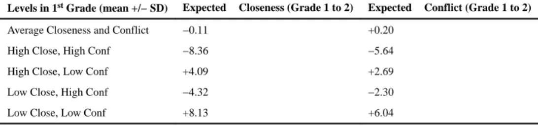
In apparent contrast, all four within-person effects from the LCS are significant and negative. Each of these effects means that higher levels predict smaller subsequent changes. However although the within-person effects are negative, the expected changes (slopes) are positive and large. Together, the changes between each pair of time points are sometimes net positive, sometimes net negative. Higher prior levels of conflict and closeness predict less change in conflict and in closeness — or even decline. A different change is expected between each set of time points, and the predicted trends form a zigzag pattern, with previous levels predicting different changes between each set of points (see Figures 4 and 5, Panel D). To understand the patterns of predicted changes, it is helpful to calculate predicted
A
uthor Man
uscr
ipt
A
uthor Man
uscr
ipt
A
uthor Man
uscr
ipt
A
uthor Man
uscr
changes based on average, high, and low levels of closeness and conflict, as in Table 4. For example, high mother-child closeness in grade 1 in the context of low conflict is associated with a predicted increase in closeness (+4.09, as opposed to a normative decrease) as well as an increase in conflict (+2.69). These differing expected changes between measurement occasions can be thought of similarly to the LCM-SR effects. The LCM-SR describes time-specific deviations from a constant slope, whereas the LCS predicts different slopes between each pair of points. Another distinction is that the effects of past changes accumulate in the LCS model. This is not true for the other models, where within-person predictions are strictly between adjacent time points.
These differences between models highlight the different conclusions about within-dyad effects that would be drawn, depending on which model was selected. The analyst who selects the ALT model, for example, would conclude that there are no bidirectional associations between closeness and conflict. The analyst who selects the LCM-SR would report a within-dyad effect of conflict on later closeness, but not the reverse. The analyst who selects the LCS model would report bidirectional effects of conflict on change in closeness, and of closeness on change in conflict.
Including Covariates
All of the discussion so far has been for unconditional models. In the LCM, person-level distal (e.g., child’s biological sex) and proximal characteristics (e.g., mother’s parenting style) can easily be incorporated as predictors of the intercepts and slopes to test hypotheses about individual differences in developmental change. For example, we could test whether trajectories of conflict differ for boys compared to girls.
As in the bivariate LCM, time-invariant covariates such as biological sex may be
incorporated into any of these models as predictors of the growth factors, permitting tests of between-person differences in the trajectories. In the LCM-SR, covariate effects are interpreted just as in the LCM. In the case of the ALT model, covariate effects describe differences in the means of the latent factors due to predictors such as biological sex, but the latent factors are still conditioned on the autoregressive and cross-lagged effects. Estimates of girls’ and boys’ mean trajectories from an ALT model, for example, represent sex differences in growth in closeness after controlling for autoregressive and cross-lagged effects. Incorporating covariates to predict the LCS growth factors shifts the expected intercept and the expected change between each set of measurements, holding cross-lagged and autoregressive effects at zero.
It is also possible to directly predict the within-person relations in each model, describing differences in the strength of the cross-lagged and autoregressive effects. For example, it is possible to test whether the within-person predictions relative to the usual trajectory in the LCM-SR differ over groups, such as women compared to men, or participants assigned to treatment versus control conditions (see Curran et al., 2014, for more discussion and a demonstration of these extensions). In sum, the approach for including predictors is similar across models, and it remains important to interpret the covariate effects according to the inferences afforded in each model.
A
uthor Man
uscr
ipt
A
uthor Man
uscr
ipt
A
uthor Man
uscr
ipt
A
uthor Man
uscr
Recommendations and Conclusions
There is no single correct strategy for modeling multivariate relationships within a person over time, yet the choice of model plays a critical role in the types of within-person inferences that can be drawn. The three modeling frameworks highlighted here emerged because scholars have differently interpreted the nature of within-person influences posited by developmental theories, and then attempted to build models capable of testing those influences. The inferences to be made from each model are overlapping but distinct, and we have sought to clarify these distinctions in order to help researchers understand the nature of different within-person inferences that can be drawn. Importantly, as shown for the present example on mother-child closeness and conflict, the conclusions drawn about within-person effects may easily differ depending on the model selected. We encourage researchers to use the summary in Table 1 to plan an analysis strategy given a particular set of research questions, harmonize seemingly contradictory results from different models, or even to apply multiple modeling strategies to the same data to gain a more comprehensive
understanding of the time-linked relations between two or more variables within a person (or dyad) over development.
Moving forward as a field into an era where data is unprecedentedly dense, we can transition from asking whether within-person relations exist to describing the nature of these relations.
Acknowledgments
This research was supported in part by award number F31DA035523 from the National Institute on Drug Abuse.
References
Baltes, PB.; Nesselroade, JR. History and rationale of longitudinal research. In: Nesselroade, JR.; Baltes, PB., editors. Longitudinal Research in the Study of Behavior and Development. New York: Academic; 1979. p. 1-39.
Bollen KA, Curran PJ. Autoregressive latent trajectory (ALT) models: A synthesis of two traditions. Sociological Methods & Research. 2004; 32(3):336–383. DOI: 10.1177/0049124103260222 Bollen, KA.; Curran, PJ. Latent Curve Models: A Structural Equation Perspective. Hoboken, NJ: John
Wiley & Sons, Inc; 2006. Multivariate latent curve models; p. 188-228.
Bronfrenbrenner, U.; Morris, PA. The Biological Model of Human Development. In: Damon, W.; Lerner, RM., editors. Handbook of Child Psychology, Volume One: Theoretical Models of Human Development. 6. New York, NY: John Wiley & Sons, Inc; 2006. p. 793-828.
Cicchetti D, Rogosch FA. Equifinality and multifinality in developmental psychology. Development and Psychopathology. 1996; 8(4):597–600. DOI: 10.1017/S0954579400007318
Clark DB, Bukstein OG. Psychopathology in adolescent alcohol abuse and dependence. Alcohol Health and Research World. 1998; 22(2):117–121. [PubMed: 15706785]
Costello EJ, Angold A, Burns BJ, Stangl D, Tweed DL, Erkanli A. The Great Smoky Mountains Study of youth: Goals, designs, methods, and the prevalence of DSM-III-R disorders. Archives of General Psychiatry. 1996; 53(12):1129–1136. DOI: 10.1001/archpsyc.1996.01830120077013 [PubMed: 8956679]
Curran PJ, Bauer DJ. The disaggregation of within-person and between-person effects in longitudinal models of change. Annual Review of Psychology. 2011; 62:583–619. 093008.100356. DOI: 10.1146/annurev.psych
Curran, PJ.; Bollen, KA. The best of both worlds: Combining autoregressive and latent curve models. In: Collins, LM.; Sayer, AG., editors. New Methods for the Analysis of Change. Washington, DC: American Psychological Association; 2001. p. 105-136.
A
uthor Man
uscr
ipt
A
uthor Man
uscr
ipt
A
uthor Man
uscr
ipt
A
uthor Man
uscr
Curran, PJ.; Lee, TH.; MacCallum, RA.; Lane, S. Disaggregating within-person and between-person effects in multilevel and structural equation growth models. In: Harring, J.; Hancock, G., editors. Advances in Longitudinal Methods in the Social and Behavioral Sciences. Charlotte, NC: Information Age; 2012.
Curran PJ, Howard AL, Bainter S, Lane SL, McGinley JS. The separation of between-person and within-person components of individual change over time: A latent curve model with structured residuals. Journal of Consulting and Clinical Psychology. 2014; 82(5):879–894. DOI: 10.1037/ a0035297 [PubMed: 24364798]
Delsing JMH, Oud JHL. Analyzing reciprocal relationships by means of the continuous-time autoregressive latent trajectory model. Statistica Neerlandica. 2008; 62:58–82.
Dodge KA, Greenberg MT, Malone PS. Conduct Problems Prevention Research Group. Testing an idealized dynamic cascade model of the development of serious violence in adolescence. Child Development. 2008; 79:1907–1927. DOI: 10.1111/j.1467-8624.2008.01233.x [PubMed: 19037957]
Dodge KA, Pettit GS. A biopsychosocial model of the development of chronic conduct problems in adolescence. Development and Psychopathology. 2003; 39(2):349–371. DOI:
10.1037//0012-1649.39.2.349
Eccles JS, Wigfield A. Motivational beliefs, values, and goals. Annual Review of Psychology. 2002; 53:109–132. DOI: 10.1146/annurev.psych.53.100901.135153
Elder, GH.; Conger, RD. Children of the Land: Adversity and Success in Rural America. Chicago: University of Chicago Press; 2002.
Ferrer E, McArdle J. Alternative structural models for multivariate longitudinal data analysis. Structural Equation Modeling. 2003; 10(4):493–524. DOI: 10.1207/S15328007SEM1004_1 Ferrer E, McArdle JJ. Longitudinal modeling of developmental changes in psychological research.
Current Directions in Psychological Science. 2010; 19(3):149–154. DOI: 10.1177/0963721410370300
Fitzmaurice, GM.; Laird, NM.; Ware, JH. Applied Longitudinal Data Analysis. 2. Hoboken, NJ: Wiley; 2011.
Gottlieb G. Experiential canalization of behavioral development: theory. Developmental Psychology. 1991; 27(1):4–13. DOI: 10.1037//0012-1649.27.1.4
Gottlieb G, Halpern CT. A relational view of causality in normal and abnormal development. Developmental Psychopathology. 2002; 27(1):4–13. DOI: 10.1017/S0954579402003024
Hoffman L, Stawski RS. Persons as contexts: Evaluating between-person and within-person effects in longitudinal analysis. Research in Human Development. 2009; 6(2–3):97–120. DOI:
10.1080/15427600902911189
Hussong AM, Huang W, Serrano D, Curran PJ, Chassin L. Testing whether and when parent
alcoholism uniquely affects various forms of adolescent substance use. Journal of Abnormal Child Psychology. 2012; 40:1265–1276. DOI: 10.1007/s10802-012-9662-3 [PubMed: 22886384] Hussong AM, Jones DJ, Stein GL, Baucom DH, Boeding S. An internalizing pathway to alcohol use
and disorder. Psychology of Addictive Behaviors. 2011; 25(3):390–404. DOI: 10.1037/a0024519 [PubMed: 21823762]
Jongerling J, Hamaker EL. On the trajectories of the predetermined ALT model: What are we really modeling? Structural Equation Modeling. 2011; 18(3):370–382. DOI:
10.1080/10705511.2011.582004
Karmiloff-Smith, A. Beyond Modularity: A Developmental Perspective on Cognitive Science. Cambridge, MA: MIT Press; 1992.
Laursen, B.; Collins, WA. Parent-child relationships during adolescence. In: Lerner, RM.; Steinberg, L., editors. Handbook of Adolescent Psychology: Volume 2: Contextual Influences on Adolescent Development. 3. Hoboken, NJ: Wiley; 2009. p. 3-42.
Lerner RM, Castellino DR. Contemporary developmental theory and adolescence: Developmental systems and applied developmental science. Journal of Adolescent Health. 2002; 31:122–135. DOI: 10.1016/S1054-139X(02)00495-0 [PubMed: 12470909]
Lerner RM, Kauffman MB. The concept of development in conceptualism. Developmental Review. 1985; 5(4):309–333.
Little, TD. Longitudinal Structural Equation Modeling. New York, NY: Guilford Press; 2013. Magnusson, D. Individual Development: A Holistic, Integrated Model. In: Moen, P.; Elder, GH.;
Luscher, K., editors. Examining Lives in Context. Washington, DC: American Psychological Association; 1995. p. 19-60.
Masten AS, Cicchetti D. Developmental cascades. Development and Psychopathology. 2010; 22(3): 491–495. DOI: 10.1017/S0954579410000222 [PubMed: 20576173]
McArdle, JJ. Dynamic but structural equation modeling of repeated measures data. In: Nesselroade, JR.; Cattell, RB., editors. The handbook of multivariate experimental psychology. Vol. 2. New York, NY: Plenum Press; 1988. p. 561-614.
McArdle, JJ. Structural modeling experiments using multiple growth functions. In: Kanfer, R.; Ackerman, P.; Cudeck, R., editors. Abilities, Motivation, and Methodology: The Minnesota Symposium on Learning and Individual Differences. Hillsdale, NJ: Lawrence Erlbaum Associates; 1989. p. 71-117.
McArdle, JJ. A latent difference score approach to longitudinal dynamic structural analysis. In: Cudeck, R.; du Toit, S.; Sorbom, D., editors. Structural Equation Modeling: Present and future. Lincolnwood, IL: Scientific Software International; 2001. p. 342-380.
McArdle JJ. Latent variable modeling of differences and changes with longitudinal data. Annual Review of Psychology. 2009; 60(1):577–605. DOI: 10.1146/annurev.psych.60.110707.163612 McArdle JJ, Epstein D. Latent growth curves within developmental structural equation models. Child
Development. 1987; 58(1):110–133. DOI: 10.2307/1130295 [PubMed: 3816341]
Meredith W, Tisak J. Latent Curve Analysis. Psychometrika. 1990; 55(1):107–122. DOI: 10.1007/ BF02294746
Molenaar PC. A Manifesto on Psychology as Idiographic Science: Bringing the Person Back Into Scientific Psychology, This Time Forever. Measurement: Interdisciplinary Research and Perspectives. 2004; 2(4):201–218. DOI: 10.1207/s15366359mea0204_1
NICHD Early Child Care Research Network. Child-care effect sizes for the NICHD study of early child care and youth development. American Psychologist. 2006; 61:99–116. DOI:
10.1037/0003-066x.61.2.99 [PubMed: 16478355]
Nesselroade, JR. The warp and woof of the developmental fabric. In: Downs, R.; Liben, L.; Palermo, D., editors. Visions of development, the environment, and aesthetics: The legacy of Joachim F. Wohlwill. Hillsdale, NJ: Erlbaum; 1991. p. 213-240.
Oud JHL. Second-order stochastic differential equation model as an alternative for the ALT and CALT models. Advances in Statistical Analysis. 2010; 94:203–215.
Paschall KW, Mastergeorge AM. A review of 25 years of research in bidirectionality in parent-child relationships: An examination of methodological approaches. International Journal of Behavioral Development. 2015; Advance online publication. doi: 10.1177/0165025415607379
Pianta, RC. The Student-Teacher Relationship Scale. Charlottesville, VA: University of Virginia; 1993. Preacher KJ. Quantifying parsimony in structural equation modeling. Multivariate Behavioral
Research. 2006; 41(3):227–259. DOI: 10.1207/s15327906mbr4103_1 [PubMed: 26750336] Preacher, KJ.; Wichman, AL.; MacCallum, RC.; Briggs, NE. Latent growth curve modeling. Thousand
Oaks, CA: Sage Publications, Inc; 2008.
Raftery AE. Bayesian model selection in social research. Sociological Methodology. 1995; 25:111– 163. DOI: 10.2307/271063
Sameroff A. A unified theory of development: a dialectical integration of nature and nurture. Child Development. 2010; 81(1):6–22. DOI: 10.1111/j.1467-8624.2009.01378.x [PubMed: 20331651] Sameroff A, MacKenzie. Research strategies for capturing transactional models of development: The
limits of the possible. Development and Psychopathology. 2003; 15(1):613–640. DOI: 10.1017/ S0954579403000312 [PubMed: 14582934]
Schulenberg, J.; Maggs, JL.; Hurrelmann, K. Negotiating developmental transitions during
adolescence and young adulthood: Health risks and opportunities. In: Schulenberg, J.; Maggs, JL.; Hurrelmann, K., editors. Health risks and developmental transitions during adolescence. New York: Cambridge University Press; 1997b. p. 1-19.
Schulenberg JE, Sameroff AJ, Cicchetti D. The transition to adulthood as a critical juncture in the course of psychopathology and mental health. Development and Psychopathology. 2004; 16(4): 799–806. DOI: 10.1017/S0954579404040015 [PubMed: 15704815]
Schulenberg, JE.; Zarrett, NR. Mental health during emerging adulthood: Continuity and discontinuity in courses, causes, and functions. In: Arnett, JJ.; Tanner, JL., editors. Emerging adults in America: Coming of age in the 21st centurv. Washington, DC: APA Books; 2006. p. 135-172.
Sliwinski M, Hoffman L, Hofer SM. Evaluating convergence of within-person change and between-person age differences in age-heterogeneous longitudinal studies. Research in Human
Development. 2010; 7(1):45–60. DOI: 10.1080/15427600903578169 [PubMed: 20671986]
A
uthor Man
uscr
ipt
A
uthor Man
uscr
ipt
A
uthor Man
uscr
ipt
A
uthor Man
uscr
Figure 1.
Bivariate Latent Curve Model
A
uthor Man
uscr
ipt
A
uthor Man
uscr
ipt
A
uthor Man
uscr
ipt
A
uthor Man
uscr
Figure 2.
Partial Equations to Illustrate Between-person and Within-person Portions of each Model in Relationship to a Standard Latent Curve Model. Note: not scaled to reflect exact amounts of variability in each model.
A
uthor Man
uscr
ipt
A
uthor Man
uscr
ipt
A
uthor Man
uscr
ipt
A
uthor Man
uscr
Figure 3.
Bivariate Autoregressive Latent Trajectory (ALT) Model
A
uthor Man
uscr
ipt
A
uthor Man
uscr
ipt
A
uthor Man
uscr
ipt
A
uthor Man
uscr
Figure 4.
Example implied trajectories of mother-child closeness from each model. The solid and dotted line represent trajectories for two randomly selected individuals, plotted along with their raw data.
A
uthor Man
uscr
ipt
A
uthor Man
uscr
ipt
A
uthor Man
uscr
ipt
A
uthor Man
uscr
Figure 5.
Example implied individual trajectories for mother-child conflict from each model. The solid and dotted line represent trajectories for two randomly selected individuals, plotted along with their raw data.
A
uthor Man
uscr
ipt
A
uthor Man
uscr
ipt
A
uthor Man
uscr
ipt
A
uthor Man
uscr
Figure 6.
Bivariate Latent Curve Model with Structured Residuals (LCM-SR)
A
uthor Man
uscr
ipt
A
uthor Man
uscr
ipt
A
uthor Man
uscr
ipt
A
uthor Man
uscr
Figure 7.
Bivariate Latent Change Score Model
A
uthor Man
uscr
ipt
A
uthor Man
uscr
ipt
A
uthor Man
uscr
ipt
A
uthor Man
uscr
A
uthor Man
uscr
ipt
A
uthor Man
uscr
ipt
A
uthor Man
uscr
ipt
A
uthor Man
uscr
ipt
Table 1
Example research questions: How are z and y related within an individual over time?
LCM ALT LCM-SR LCS
Between-person
Is the starting point or rate of change in z related to the starting point or rate of change in y? ✓ ✓
Within-person
Is the starting point or rate of change in z related to the starting point or rate of change in y, after
controlling for time-specific deviations from a linear trajectory? ✓
When z is higher than usual*, does y tend to be higher (or lower) than usual? ✓ ✓ ✓ ✓ Do deviations from a linear trajectory of z predict deviations from a linear trajectory of y? ✓
Do higher-than-usual* levels of z at one wave predict higher-(or lower) than-usual* levels of y at the next
wave? ✓
In the relationship between z and y over time, is one variable leading? ✓ ✓
Does the level of z at one wave predict (more/less) subsequent change in y? ✓ Note.
*
A
uthor Man
uscr
ipt
A
uthor Man
uscr
ipt
A
uthor Man
uscr
ipt
A
uthor Man
uscr
ipt
Table 2
Overall Fit of Bivariate Models of Mother Closeness and Mother Conflict (N = 849)
Fit Statistic LCM ALT LCM-SR LCS
RMSEA (90% C.I.) .060 (.051, .069) .049 (.038, .060) .046 (.036,.056) .066 (.057, .075) Chi-Square 192.95(48) 94.13 (31) 118.08 (42) 208.00 (44)
CFI/TLI .973/.974 .988/.983 .986/.985 .969/.968 BICk −130.76 −114.94 −165.18 −88.74
A
uthor Man
uscr
ipt
A
uthor Man
uscr
ipt
A
uthor Man
uscr
ipt
A
uthor Man
uscr
ipt
Table 3
Selected Estimates from Models of Mother-Child Closeness and Mother-Child Conflict (N = 849)
Parameter LCM ALT LCM-SR LCS
Mother-child closeness
Mean intercept μyα 38.0 (.08) 38.2(.14) 38.0 (.08) 37.9 (.08)
Mean slope μyβ −0.36 (.02) −0.47 (.05) −0.36 (.02) 46.3 (9.6)
Intercept variance ψ11 2.98 (.29) 5.00 (.79) 2.99 (.34) 2.62 (.29)
Slope variance ψ22 0.14 (.02) 0.25 (.06) 0.12 (.02) 23.7 (9.6)
Int/slope covariance ψ21 0.25 (.06) −0.23 (.18) −0.23 (.07) −0.60 (.63)
Residual variance
3.70 (.10) 3.55 (.13) 3.98 (.14) 3.64 (.11)
Mother-child conflict
Mean intercept μzα 15.2 (.20) 15.4 (.28) 15.2 (.20) 15.2 (.20)
Mean slope μ̂zβ 0.30 (.04) 0.38 (.08) 0.30 (.04) 36.0 (8.2)
Intercept variance ψ33 25.7 (1.6) 38.5 (3.2) 24.2 (1.7) 24.1 (1.5)
Slope variance ψ44 0.40 (.06) 0.99 (.17) 0.26 (.07) 11.5 (5.8)
Int/slope covariance ψ43 −0.57 (.23) −3.47 (.60) −0.29 (.28) 13.5 (4.6)
Residual variance
9.90 (.28) 8.79 (.39) 11.0 (.39) 10.6 (.31)
Growth curve covariances
Int/int covariance ψ31 −3.87 (.51) −2.69 (1.2) −3.96 (.52) −4.18 (.49)
CLOSE int/CONF slope ψ41 0.13 (.09) −0.10(.29) −0.16 (.09) 0.01 (.54)
CONF int/CLOSE slope ψ32 −0.41 (.13) −3.10 (.70) −0.43 (.13) 20.8 (4.7)
Slope/slope covariance ψ42 −0.07 (.02) −0.04 (.09) −0.07 (.03) 16.2 (2.9)
Within-person effects
Contemporaneous σezy −1.31 (.12) −1.37 (.16) −1.32 (.16) −1.20 (.12)
CLOSE autoreg ρyy, ρòyy — 0.01 (.01) 0.14 (.03) −0.80 (.18)
CONF autoreg ρzz, ρezz — 0.02 (.03) 0.22 (.04) −0.71 (.19)
Cross-lag CONF→CLOSE ρ̂yz, ρ̂eyz — −0.001 (.01) 0.04 (.02) −1.06 (.21)
Cross-lag CLOSE ρ̂zy, ρ̂ezy — −0.02 (.01) 0.02 (.05) −0.66 (.16)