SIMULATION AND LEARNING FOR URBAN MOBILITY: CITY-SCALE TRAFFIC RECONSTRUCTION AND AUTONOMOUS DRIVING
Weizi Li
A dissertation submitted to the faculty of the University of North Carolina at Chapel Hill in partial fulfillment of the requirements for the degree of Doctor of Philosophy in the Department of Computer Science.
Chapel Hill 2019
© 2019 Weizi Li
ABSTRACT
Weizi Li: Simulation and Learning for Urban Mobility: City-scale Traffic Reconstruction and Autonomous Driving
(Under the direction of Ming C. Lin)
Traffic congestion has become one of the most critical issues worldwide. The costs due to traffic gridlock and jams are approximately $160 billion in the United States, more than £13 billion in the United Kingdom, and over one trillion dollars across the globe annually. As more metropolitan areas will experience increasingly severe traffic conditions, the ability to analyze, understand, and improve traffic dynamics becomes critical. This dissertation is an effort towards achieving such an ability. I propose various techniques combining simulation and machine learning to tackle the problem of traffic from two perspectives: city-scale traffic reconstruction and autonomous driving.
Traffic, by its definition, appears in an aggregate form. In order to study it, we have to take a holistic approach. I address the problem of efficient and accurate estimation and reconstruction of city-scale traffic. The reconstructed traffic can be used to analyze congestion causes, identify network bottlenecks, and experiment with novel transport policies. City-scale traffic estimation and reconstruction have proven to be challenging for two particular reasons: first, traffic conditions that depend on individual drivers are intrinsically stochastic; second, the availability and quality of traffic data are limited. Traditional traffic monitoring systems that exist on highways and major roads can not produce sufficient data to recover traffic at scale. GPS data, in contrast, provide much broader coverage of a city thus are more promising sources for traffic estimation and reconstruction. However, GPS data are limited by their spatial-temporal sparsity in practice. I develop a framework to statically estimate and dynamically reconstruct traffic over a city-scale road network by addressing the limitations of GPS data.
ACKNOWLEDGMENTS
First of all, I would like to thank my advisor, Ming C. Lin, who has and continues to support me during my time at UNC and has taught me numerous lessons regarding academic life and beyond. I also want to express my sincerest appreciation to the rest of my committee members: Dinesh Manocha, Julien Pettr´e, Ron Alterovitz, and David Wilkie.
My research will not advance without wonderful collaborators I have had in years. Among them, I want to express my deep gratitude to David Wolinski, who has been serving as my mentor and behind all my important projects, and Jan Allbeck, who had led me to the wonderful research world. I am also thankful to all my supervisors at various institutes: Ellen Yi-Luen Do, Xiang Cao, and Carol O’Sullivan for their guidance and wisdom.
It has been a great pleasure to work in the GAMMA research lab and interact with its amazing members. I would like to especially thank Shan Yang, Auston Sterling, Tetsuya Takahashi, Andrew Phillip Best, Aniket Bera, Sujeong Kim, Chonhyon Park, Junbang Liang, and Zhenyu Tang for their help and companionship.
My life at Chapel Hill has been an enjoyable adventure because of the friends I made across the campus. This list includes but not limited to: Yingchi Liu, Xin Zhao, Fan Jiang, Xuxiang Mao, Jun Jiang, Dong Nie, Licheng Yu, Qishun Tang, Feng Shi, Yan Song, Meilei Jiang, Yaoyu Chen, Jiangyue Sun, Chuyi Du, Yunyan He, Zhaopeng Xing, Zhechang Yuan, Yang Zhan, and Tao Zhang. Thank you for sharing this adventure with me at UNC!
TABLE OF CONTENTS
LIST OF TABLES . . . xi
LIST OF FIGURES . . . xii
1 INTRODUCTION . . . 1
1.1 City-Scale Traffic Reconstruction . . . 2
1.2 Autonomous Driving . . . 4
1.3 Main Results . . . 7
1.3.1 City-Scale Traffic Reconstruction . . . 7
1.3.1.1 Deterministic Estimation of Traffic Conditions . . . 7
1.3.1.2 Temporal Missing Data Completion . . . 9
1.3.1.3 Iterative Estimation and Spatial Missing Data Completion . . . 13
1.3.2 Autonomous Driving . . . 18
1.3.2.1 Theoretical Results . . . 21
1.3.2.2 Experimental Results . . . 22
1.4 Thesis Statement . . . 25
1.5 Organization . . . 25
2 CITYWIDE ESTIMATION OF TRAFFIC DYNAMICS VIA SPARSE GPS TRACES . . . 26
2.1 Introduction. . . 26
2.2 Related Work . . . 29
2.3 Traffic Velocity Field Reconstruction . . . 30
2.3.1 Notation and Definitions . . . 30
2.3.3 Travel Time Allocation . . . 35
2.3.4 Evaluation on A Synthetic Network Using Traffic Simulation . . . 38
2.4 Missing Value Completion . . . 40
2.5 Estimating Traffic Dynamics Via GPS Data . . . 46
2.6 Summary and Future Work . . . 48
3 CITY-SCALE TRAFFIC ANIMATION USING STATISTICAL LEARNING AND METAMODEL-BASED OPTIMIZATION . . . 50
3.1 Introduction. . . 50
3.2 Related Work . . . 52
3.3 Overview . . . 54
3.3.1 System . . . 54
3.3.2 Notation . . . 56
3.4 City-Scale Traffic Reconstruction . . . 57
3.4.1 Initial Estimation . . . 58
3.4.2 Iterative Estimation . . . 59
3.4.2.1 Map Matching . . . 59
3.4.2.2 Travel Time Estimation . . . 59
3.4.3 Bilevel Optimization . . . 60
3.5 Dynamic Data Completion. . . 62
3.5.1 Metamodel-Based Simulation Optimization . . . 63
3.5.2 Algorithmic Steps . . . 65
3.6 Results . . . 66
3.6.1 Evaluation of Initial Traffic Reconstruction . . . 66
3.6.1.1 Road Network and GPS Dataset . . . 67
3.6.1.2 Traffic Conditions via System Optimal Model . . . 67
3.6.1.3 Traffic Conditions via Timestamp Model . . . 68
3.6.1.6 Analysis of Bilevel Optimization . . . 73
3.6.2 Evaluation of Dynamic Data Completion . . . 73
3.6.3 Traffic Visualization and Animation . . . 75
3.7 Summary and Future Work . . . 79
4 ADAPS: AUTONOMOUS DRIVING VIA PRINCIPLED SIMULATIONS . . . 81
4.1 Introduction. . . 81
4.2 Related Work . . . 82
4.3 Preliminaries . . . 83
4.4 ADAPS . . . 90
4.4.1 Theoretical Analysis . . . 90
4.4.2 Framework Pipeline . . . 93
4.5 Policy Learning . . . 93
4.5.1 End-to-end Imitation Learning . . . 94
4.5.2 Training Data Collection . . . 95
4.6 Learning from Accidents . . . 95
4.6.1 Solving Accidents . . . 95
4.6.2 Additional Data Coverage . . . 96
4.7 Experiments . . . 99
4.7.1 Experiment Setup . . . 99
4.7.1.1 Scenarios . . . 99
4.7.1.2 Vehicle Specifications . . . 100
4.7.1.3 Obstacles . . . 100
4.7.1.4 Training Data . . . 100
4.7.2 Evaluation Results . . . 101
4.7.2.1 On-road Scenarios . . . 101
4.7.2.2 Off-road Scenario . . . 103
4.8 Summary and Future Work . . . 103
5 CONCLUSION . . . 106
5.1 Summary of Results . . . 106
5.2 Future Work . . . 108
5.2.1 Macroscopic Level . . . 108
5.2.2 Microscopic Level . . . 109
5.2.3 Connection Between The Two Levels . . . 110
LIST OF TABLES
1.1 The absolute errors in the recovered travel time computed using my technique vs. Lou et al. (Lou et al., 2009) by using GPS traces from various percentages of the traffic population. My technique results in much smaller errors as of Lou et
al. (Lou et al., 2009). . . 9 1.2 Test Results of On-Road Scenarios: my policies Ostraight &Of ull can lead to
robust collision avoidance and lane-following behaviors. . . 23
2.1 The absolute errors in the recovered travel times computed using my technique vs. Lou et al. (Lou et al., 2009), using GPS traces from various percentages of the traffic population. My technique results in much smaller errors as of Lou et
al. (Lou et al., 2009). . . 39
4.1 Training Data Summary: my method can achieve over 200 times more training examples than DAGGER (Ross et al., 2011) at one iteration leading to large
improvements of a policy. . . 102 4.2 Test Results of On-Road Scenarios: my policies Ostraight &Of ull can lead to
LIST OF FIGURES
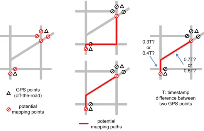
1.1 Illustrations of procedures required to process GPS data for traffic estimation and reconstruction. LEFT (map-matching): off-the-road GPS points need to be mapped onto a road network. MIDDLE (map-matching): after determining the matching points, the traversed path of a vehicle needs to be inferred. RIGHT (travel-time estimation): after determining the traversed path, the timestamp difference needs
to be distributed to individual road segments. . . 3 1.2 Illustration of the sparsity issue embedded in GPS data. One-day GPS data of
downtown San Francisco from the Cabspotting project (Piorkowski et al., 2009)
are plotted, marked regions showing the lack of data. . . 4 1.3 Recovery of average travel time on different percentages of the traffic population
using my approach (TOP) vs. Lou et al. (Lou et al., 2009) (BOTTOM). My technique consistently outperforms Lou et al. (Lou et al., 2009) in estimating the
average travel time over 30 different congestion levels. . . 8 1.4 Relative improvements measured in MSE of my technique over Lou et al. (Lou
et al., 2009) on travel time. My technique outperforms Lou et al. (Lou et al., 2009) as the congestion level increases or as more GPS traces become available for the
recovery task. . . 10 1.5 The average speed measurements from loop-detector data are interpreted as atraffic
signal, which exhibits a clear periodic pattern (TOP); the spectral analysis reveals that the most prominent frequency is one cycle per day (i.e., 24 hours) (MIDDLE); the traffic signal is approximated by a frequency-domain linear regression model
in which 95% energy is retained by keeping the 10 largest frequencies (BOTTOM). . . 11 1.6 The top panel shows the decaying rates of frequency magnitudes of all traffic
signals; the bottom panel shows the locations and normalized magnitudes of the frequency components of all traffic signals. The rapid growth of decaying rates and randomly distributed frequency structures indicate that Compressed Sensing is
applicable for recovering a traffic signal. . . 12 1.7 A recovered traffic signal using my technique highly resembles its original form. . . 13 1.8 My technique shows robustness when the number of samples used in recovering a
traffic signal decreases. . . 14 1.9 Estimated traffic pattern of downtown San Francisco (TOP) and its spectral analysis
(BOTTOM). The result from my technique demonstrates a clear daily trend, which
1.10 Correlation between every pair of days in a week. The left panel lists normalized similarity scores calculated using the cosine distance, and the right panel provides the qualitative results. For both, the upper triangular matrix is derived using the estimated traffic conditions from GPS data, and the lower triangular matrix is computed using loop-detector data from the same area. When data and patterns are compared across the diagonal line, my estimated results exhibit high similarity to
the loop-detector data. . . 15 1.11 My algorithm on map-matching and travel-time estimation achieves consistent
improvements over the previous techniques (Rahmani et al., 2015; Hunter, 2014)
in various measures. . . 16 1.12 The error level of my technique vs. simulation-only approach: For a given road
network and a specific origin-destination demand, I first compute the differences between the two methods with respect to the ground truth. Then, I subtract these two differences to obtain one error difference measure (indicated by a gray cross). The mean, minimum, and maximum values of the average error level (indicated by the solid line) are respectively 7.8%, 0%, and 13%. In many cases, my technique even outperforms the simulation-only approach with much smaller differences to
the ground truth, shown by the negative values. . . 17 1.13 The performance speedup of my technique over the simulation-only approach:
my technique ison average about27.2x faster, with maximum and minimum performance gains of35.6xand16.1x. The maximum observed performance gain
of a single speedup measure isover90x(at origin-destination demand = 9000). . . 17 1.14 2D traffic animation of regions in San Francisco: Northeast (top left), Central-East
(top center), Central (top Right), Northwest (bottom). I have exaggerated the headlights and adopted an evening time period (i.e., Friday 7PM) to make vehicles
more visible. . . 18 1.15 3D traffic animation: a perspective overview (left), a topdown view (center), and a
driver’s view (right). . . 18 1.16 Visualization of traffic patterns in San Francisco and Beijing. Four time periods of
a week, namely Sunday 9AM, Tuesday 9AM, Thursday Noon, and Friday 7PM, are selected to illustrate weekend vs. weekday and morning vs. evening traffic. The traffic is measured by Volume Of Capacity (VOC). All computations are conducted
in epoch time. . . 19 1.17 The estimated traffic conditions measured in average volume over capacity (VOC)
of San Francisco and Beijing for various types of roads. All computations are con-ducted in epoch time. My technique successfully recovers the periodic phenomena in all cases. In San Francisco, saddle shapes appear onmotorway and truckand overall roads for several days indicating mid-day traffic relief. Such phenomena are not observed in Beijing, which suggests the similar usage of different types of
1.18 LEFT and CENTER: the comparisons between my policyOf ull(TOP) and Bojarski et al. (Bojarski et al., 2016),Bf ull (BOTTOM).Bf ull causes collision whileOf ull steers the AV away from the obstacle. RIGHT: the accident analysis results on the open ground. I show the accident caused by an adversary vehicle (TOP); then I
show, after additional training, the AV can avoid the adversary vehicle (BOTTOM). . . 23 1.19 The visualization results of collected images using t-SNE (Maaten and Hinton,
2008). My method generates more heterogeneous training data compared to
DAGGER (Ross et al., 2011) in one learning iteration. . . 24
2.1 Pipeline of my framework. Map Matching and Travel Time Allocation are applied on individual time intervals, while Missing Value Completion is performed over
all time intervals. . . 28 2.2 An example illustrating a failure using the shortest distance criterion for
map-matching traceStoT1,T2, orT3. LEFT: By matching travel time of traceSand road conditions, the correct pathT1is identified. RIGHT: By only considering the
shortest distance path,Sis mismatched toT3. . . 31 2.3 An illustration of the relaxation process of two tracesS1andS2. The actual traffic
conditions and trace matching results are shown in the TOP-LEFT panel. The input listed in the TOP-RIGHT panel contains the initial network and trace information (i.e., sources, targets, and travel time). After relaxation of traceS1, pathsT1and T3have their travel times increased toS1.t. WhileS1can be matched to either T1orT3, the situation is resolved after relaxation ofS2due to further increase in
the travel time of the road segmente. . . 34 2.4 Recovery of average travel time on different percentages of the traffic population
using my approach (TOP) vs. Lou et al. (Lou et al., 2009) (which uses the shortest-distance criterion) (BOTTOM). My technique consistently outperforms Lou et al. (Lou et al., 2009) in estimating the average travel time over 30 different
congestion levels. . . 39 2.5 Relative improvements measured in MSE of my technique over Lou et al. (Lou
et al., 2009). My technique outperforms Lou et al. (Lou et al., 2009) as the
congestion level increases or more GPS traces become available in estimation. . . 40 2.6 The average speed measurements from a loop detector are interpreted as atraffic
signal, which exhibits a clear periodic pattern (TOP); the spectral analysis reveals that the most prominent frequency is one cycle per day (MIDDLE); the traffic signal is approximated by a frequency-domain linear regression model, in which
95% energy is retained by keeping the 10 largest frequencies (BOTTOM). . . 42 2.7 The top panel shows the decaying rates of frequency magnitudes of all traffic
signals; the bottom panel shows the locations and normalized magnitudes of the frequency components of all traffic signals. The rapid growth of decaying rates and randomly distributed frequency structures indicate that Compressed Sensing is
2.8 Solution elements (in total 168) by solving an underdetermined system via convex optimization. Both the actual and theL1-norm based recovery demonstrate sparsity
(i.e., most solution elements are approximately zero). . . 44 2.9 Recovery of a traffic signal via Compressed Sensing. The actual signal and its 90
random measurements are plotted (TOP). TheL1-norm based recovery (BOTTOM)
shows high similarity to the actual signal.. . . 45 2.10 Errors between recovered and actual traffic signals. As more samples are used in
signal’s recovery, smaller errors are observed. This analysis also demonstrates the robustness of my approach as the error only increases linearly when the number of
samples used in recovery decreases. . . 46 2.11 Estimated traffic pattern of downtown San Francisco using the Cabspotting dataset
(Pi-orkowski et al., 2009) (TOP) and its corresponding spectral analysis (BOTTOM). The recovery from my technique shows a clear daily trend, which is consistent
with the features observed in loop-detector data from the same area. . . 47 2.12 Correlation between every pair of days in a week. The left panel lists the normalized
similarity scores calculated using the cosine distance, and the right panel provides the qualitative results. In both, the upper triangular matrix is derived using the estimated traffic conditions, and the lower triangular matrix is computed using loop-detector data from the same area. When data and patterns are compared across the diagonal line, my estimated results exhibit high similarity to the loop-detector
data. . . 48
3.1 The systematic view of my framework. Trip records are optional as they can be
inferred from GPS traces on a digital map. . . 55 3.2 LEFT: Sample GPS points from the Cabspotting dataset. MIDDLE: Road maps of
downtown San Francisco overlaid with traffic analysis zones (TAZs). RIGHT: A heuristic traffic condition established via the Timestamp model (the travel times
are converted to flows). . . 67 3.3 The relationship between the normalized convergence rate and the number of
iterations of the outer loop of my iterative process is shown. The convergence rate decreases quadratically as the number of iterations increases and tends to flat after
10 iterations. . . 69 3.4 From TOP to BOTTOM, the left diagrams show the results generated using network
travel times via the system optimal (SO) model, while the right diagrams show corresponding results of network travel times via the Timestamp model. TOP: The error rates (%) of various methods of aggregating travel time across the network. MIDDLE: The relative improvements (%) of travel times of all road segments measured in MSE. BOTTOM: The relative improvements (%) of map-matching accuracy measured using successfully identification rates of road segments. In summary, my technique achieves consistent improvements over the other two
3.5 TOP and MIDDLE: The normalized noisy levels (%) of target road-segment flows ¯
f computed according to the MSE of estimated network travel times to ground truth. In general, for both models, my technique produces lower noisy levels than the other two techniques. BOTTOM: The normalized MSE of target OD pairsuˆ (%) under different values of the weighting factorηand various noisy levels of¯f (%). Whenηis small, the error is more sensitive to perturbations on¯f. Overall, the error increases as the noisy level of¯fincreases. For all studies, the normalized noisy level of target OD pairsu¯ has been set to50%. My method has achieved
consistently lower error rates compared to the other two methods. . . 72 3.6 The error level of my technique vs. simulation-only approach: For a given road
network and a specific OD demand, I first compute the differences between the two methods with respect to the ground truth. Then, I subtract these two differences to obtain one error difference measure (indicated by a gray cross). The mean, minimum, and maximum values of the average error level (indicated by the solid line) are respectively 7.8%, 0%, and 13%. In many cases, my technique even outperforms the simulation-only approach with a smaller difference to the ground
truth, as indicated by a negative value in the diagram. . . 74 3.7 The performance speedup of my technique over the simulation-only approach:
my technique ison average about27.2x faster, with maximum and minimum performance gains of35.6xand16.1x. The maximum observed performance gain
of a single speedup measure isover 90x(at OD demand = 9000). . . 75 3.8 (a) TOP: several loop-detector signals are plotted showing phase shifts among
them; BOTTOM: the average signal of the signals shown in the top panel. (b) TOP: aligned loop-detector signals according to their phase responses; BOTTOM: the average signal of the aligned signals shown in the TOP panel. (c) TOP: the averaged frequency of the signals in (a) TOP, which shows several frequency component are getting degraded; MIDDLE: the frequency of the signal in (a) BOTTOM, which shows inconsistent magnitude ratios; BOTTOM: the frequency of signal in (b)
BOTTOM, which shows prominent frequencies and magnitude ratios. . . 76 3.9 Qualitative (visualization) and quantitative analysis of traffic in San Francisco.
Top: four time periods, namely Sunday 9AM, Tuesday 9AM, Thursday Noon, and Friday 7PM, are adopted to illustrate weekend vs. weekday and morning vs. evening traffic. The traffic is measured byvolume over capacity(VOC) (computed asP
e∈E(f(e)/c(e))wherec(e)is the capacity of the road segmentedefined in
Equation 3.11). Bottom: I compare my reconstructed results using GPS data (after the filtering process explained in this section) to the data from three loop detectors
in San Francisco. The results show small losses (around1m/s) in the speed measurement. . . 77 3.10 2D traffic animation of regions in San Francisco: Northeast (top left), Central-East
(top center), Central (top Right), Northwest (bottom). I have exaggerated the headlights and adopted an evening time period (i.e., Friday 7PM) to make vehicles
4.1 Collision-free trajectories generated by the expert algorithm for a vehicle traveling on the right lane of a straight road, with an obstacle in front: in total, 74 trajectories span from the first moment the vehicle perceives the obstacle (green, progressive
avoidance) to the last moment the collision can be avoided (red, sharp avoidance). . . 97 4.2 Illustration of important points and DANGER/SAFE labels from Section 4.6 for
a vehicle traveling on the right lane of a straight road, with an obstacle in front. Labels are shown for four points{lu1,lu2,lu3,lu4}illustrating the four possible
cases. . . 97 4.3 LEFT and CENTER: the comparisons between my policyOf ull(TOP) and Bojarski
et al. (Bojarski et al., 2016),Bf ull (BOTTOM).Of ullcan steer the AV away from the obstacle whileBf ull causes collision. RIGHT: the accident analysis results on the open ground. I show the accident caused by an adversary vehicle (TOP); then I
show after additional training the AV can avoid the adversary vehicle (BOTTOM). . . 101 4.4 The visualization results of collected images using t-SNE (Maaten and Hinton,
2008). My method can generate more heterogeneous training data compared to DAGGER (Ross et al., 2011) in one learning iteration as the sampled trajectories
CHAPTER 1: INTRODUCTION
Throughout history, human mobility not only characterizes our way of life but also plays an essential role in socio-economic development. In the past century, as a result of rapid motorization and urbanization, increasing human-mobility patterns are stemmed from automobiles and are appearing in urban environments. While this phenomenon reflects better accessibility to societal resources and an increase in quality of life, the resulting traffic congestion has become one of the most infamous problems across the globe. The annual costs due to traffic gridlock and jams are nearly $160 billion in the U.S., £13 billion in the U.K., and exceeding one trillion U.S. dollars worldwide.
As urbanization, motorization, and vehicle production rates keep climbing—especially in Asia and Africa—we will witness many more metropolitan areas forming, growing, and experiencing severe traffic conditions. The ability to understand and improve traffic dynamics is thus critical more today than ever.
Traffic can be studied at various scales. Traffic is an aggregate phenomenon, which can appear at a large spatial-temporal scale. Study of its dynamics requires a holistic view. Among various traffic engineering tasks, one crucial task is the efficient and accurate estimation and reconstruction of city-scale traffic. This task can enable many Intelligent Transportation System (ITS) applications such as identifying congestion causes, detecting network bottlenecks, planning traffic flows, and analyzing transport policies.
Additionally, traffic is formed by individual vehicles propagating through space and time. If we can improve the efficiency and coordination of them, jointly, we have the opportunity to alleviate severe traffic conditions in metropolitan areas. While the behaviors of human-driven vehicles can be only altered through regulations and policies, the behaviors of autonomous vehicles can be precisely directed and optimized via control algorithms. Thus, the switch from human-driven vehicles to autonomous vehicles has the potential to revolutionize our transportation systems by reducing the number of crashes and alleviating traffic jams which both, by a large degree, attribute to human factors.
and machine learning techniques for distilling travel patterns from a large volume of traffic data in order to estimate and reconstruct traffic at a metropolitan scale. Microscopically, I studyautonomous driving: I have developed simulation platforms and an online learning mechanism for effectively and efficiently learning and testing control policies for autonomous driving.
1.1 City-Scale Traffic Reconstruction
In order to analyze congestion causes, identify network bottlenecks, and experiment with novel transport policies, we need to be able to reconstruct and simulate city-scale traffic at the macroscopic level. I have developed methods to efficiently and accurately estimate and reconstruct large-scale traffic using mobile-sensor data while generating visual analytics in various forms.
Estimation and reconstruction of large-scale traffic is difficult due to fundamental challenges: 1) traffic dynamics is intrinsically stochastic as a result of individual drivers’ behaviors, and 2) the availability and quality of traffic data are usually limited. Conventionally, traffic data are collected via in-road sensors such as loop detectors and video cameras. While these sensors produce accurate measurements, they are mostly installed on highways and major roads, which only constitute a small portion of a city. Mobile-sensor data, such as GPS reports, are more promising sources for the estimation and reconstruction task due to their broader coverage. However, GPS points usually embed a low-sampling rate, meaning that the time lapse between two consecutive reports is large (e.g., greater than 60 seconds), and exhibit spatial-temporal sparsity, meaning that the data are scarce in certain areas and time periods.
In order to adopt GPS data for reconstructing full traffic dynamics, several procedures are required to address the abovementioned features: 1)map-matching, which maps off-the-road GPS points (due to inevitable measurement noise) onto a road network and infers the traversed path of a vehicle (illustrated in Figure 1.1 LEFT and MIDDLE); 2)travel-time estimation, which estimates the travel time of a road network through GPS timestamps (illustrated in Figure 1.1 RIGHT); 3)missing-data completion, which interpolates spatial-temporal missing measurements (illustrated in Figure 1.2).
Figure 1.1: Illustrations of procedures required to process GPS data for traffic estimation and reconstruction. LEFT matching): off-the-road GPS points need to be mapped onto a road network. MIDDLE (map-matching): after determining the matching points, the traversed path of a vehicle needs to be inferred. RIGHT (travel-time estimation): after determining the traversed path, the timestamp difference needs to be distributed to individual road segments.
the latter is preferred by GPS devices and experienced drivers. If we adopt a sequential pipeline to process GPS data,travel-time estimation(the subsequent step ofmap-matching) will produce inaccurate results, since the timestamp difference between GPS reports will be distributed to a wrong set of road segments.
Figure 1.2: Illustration of the sparsity issue embedded in GPS data. One-day GPS data of downtown San Francisco from the Cabspotting project (Piorkowski et al., 2009) are plotted, marked regions showing the lack of data.
Chapter 2 and Chapter 3 are dedicated to address the limitations of GPS data and explain how to accurately and efficiently estimate traffic conditions, interpret spatial-temporal missing traffic data, and dynamically reconstruct traffic flows at a city scale.
1.2 Autonomous Driving
While traffic dynamics can only be studied collectively, it is also formed by individual vehicles. Given over 90% crashes are due to human errors, the conversion from human-driven vehicles to autonomous vehicles (AVs)—with improved safety and efficiency features—has the potential to alleviate the severe traffic conditions (Wu et al., 2018).
Widespread research on autonomous driving has been conducted as a result of recent advancements in automation and machine learning algorithms. Before the deployment of AVs, we need to scrutinizingly test and improve their safety, control, and coordination. I have developed a framework, named ADAPS (AutonomousDriving Via PrincipledSimulations), which not only can be used to simulate, analyze, and produce driving data in various scenarios including accidents, but also represent a more efficient online learning mechanism for learning robust control policies for autonomous driving (Li et al., 2019).
be used to model the cost of an action at each time step and consequences of an action in the future (Ratliff, 2009; Silver, 2010). Describing and parameterizing an uncontrolled and unpredictable driving environment is a daunting and often impractical task, thus preventing the conventional techniques from succeeding.
Nevertheless, driving, as a complex task, can be easily demonstrated by humans. The intricate traffic flow manifests such success. This phenomenon has inspiredimitation learning—a data-driven machine learning technique that leverages expert demonstrations to synthesize a controller for achieving a desired behavior. A number of studies have shown that imitation learning is an effective approach capable of learning policies for a juggling robot (Atkeson, 1994), a quadruped robot maneuvering on rough terrains (Ratliff et al., 2007), and autonomous driving on highway (Pomerleau, 1989), among many others.
A straightforward way to achieve imitation learning is via standard supervised learning: learning a training dataset that is a collection of observations and their corresponding behaviors. In the context of driving, this training dataset could be images from a front-facing camera and the steering angle applied while each image was taken. The effectiveness of supervised learning is commonly shown by running a learned model on a test dataset and analyzing the results.
Supervised learning operates based on one assumption—the examples in both training and test datasets are independently and identically distributed (i.i.d.) (Friedman et al., 2001). While this assumption is reasonable for many problems, it fails to apply on driving, in which task the training and test examples are not i.i.d. (Ross et al., 2011).
To be specific, autonomous driving is a sequential prediction and controlled (SPC) task, meaning the system has to predict a sequence of control commands over time to achieve a goal. Given the sequential nature, in such a system, any predicted control commands will affect the following observations being taken by the system and, consequently affect the future predicted control commands (since the predictions are drawn based on the observations). Because the predictor and the observer are entangled, their resulting training and test examples violate the i.i.d. assumption.
confuse the control module, causing an unpredictable maneuver of the vehicle and lead the vehicle to more “unseen” observations. This mismatch between the observations used for training (i.e., training distribution) and the observations encountered during testing (i.e., test distribution) is termedcovariate shift(Sugiyama and Kawanabe, 2012).
In essence, a driving policy from supervised learning by treating all training examples as i.i.d. will not be robust to its own mistakes and likely lead a vehicle to dangerous situations including accidents. To alleviate this issue, first, we need driving data from both safe and, especially, dangerous situations. This is critical because most expert demonstrations (i.e., human driving data) are from safe driving. However, if a learning algorithm is not trained on recovery demonstrations in dangerous situations, when encountering, the algorithm’s behavior is undefined. Second, we need an efficient online learning mechanism. For solving an SPC task, interactions with experts in a number of iterations are essential, without which, no learning algorithm can ensure robust performance (Ross et al., 2011). Since learning an effective policy for an SPC task requires iterative testing and update, an efficient online learning technique that can reduce the number of learning iterations is desired. For autonomous driving, this becomes critical given that one iteration implies one incident (otherwise there is no need to update a policy by proceeding to the next iteration). Third, we need an effective architecture for the control policy. In the simplest case, a policy needs to classify road conditions and make corresponding maneuvers. The two basic road conditions are “safe”, e.g., no obstacle on the road—the vehicle can just follow the road, and “dangerous”, e.g., an obstacle appearing on the road—the vehicle needs to avoid it. Next, I will briefly explain and introduce my solutions to these challenges.
Obtaining recovery data of vehicles from dangerous situations in the physical world is impractical, due to the high expenditure of a vehicle and potential injuries to people both inside and outside a vehicle. In addition, even if such recovery data are collected, human experts are usually required to label them. This process could be inefficient and subject to judgmental errors (Ross et al., 2013). These difficulties suggest the potential use of the virtual world, in which we can simulate various dangerous scenarios including accidents and then analyze the simulated scenarios to generate recovery data. I have developed a simulation platform for this purpose.
number of “expert” trajectories be generated indefinitely, but the access to such an “expert” is instantaneous. These features will assist in reducing the number of learning iterations.
Lastly, I propose a hierarchical control policy using deep neural networks (LeCun et al., 2015) and long short-term memory networks (Hochreiter and Schmidhuber, 1997). My policy consists of three modules, the
detectionmodule, which monitors a road condition and categorizes it as “safe” or “dangerous”, thefollowing
module, which directs a vehicle to follow the road if the condition is considered “safe”, and theavoidance
module, which steers a vehicle away from an obstacle when the road condition is considered “dangerous”. Chapter 4 is dedicated to explain the abovementioned solutions in details.
Although this dissertation addresses the macroscopic level and the microscopic level of traffic separately, the two levels are tightly coupled. Many applications can stem from their rich connection. For example, from macroscopic to microscopic, the reconstructed city-scale traffic can assist route planning of autonomous driving and enrich virtual environments for training purposes (Chao et al., 2019); from microscopic to macroscopic, individual autonomous vehicles can be adopted to stabilize and regulate traffic flows (Wu et al., 2018). These applications will be further discussed in Chapter 5. In the following, I will introduce the main results regardingcity-scale traffic reconstructionandautonomous driving.
1.3 Main Results
1.3.1 City-Scale Traffic Reconstruction
1.3.1.1 Deterministic Estimation of Traffic Conditions
My first solution to the estimation of traffic conditions is an efficient deterministic approach (Li et al., 2017a), for which details can be found in Chapter 2. My solution is based on two observations: traffic patterns exhibit weekly periodicityandtraffic conditions are quasi-static. Using these observations, I treat one week as a traffic period and assume that traffic conditions are static within each hourly time interval of a weekly period. Then, in each time interval, I conductmap-matchingby replacing the shortest distance criterion with the shortest travel-time criterion, since the former criterion can lead to mapping errors in a congested network.
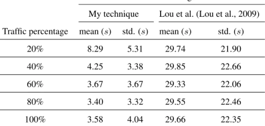
Figure 1.3: Recovery of average travel time on different percentages of the traffic population using my approach (TOP) vs. Lou et al. (Lou et al., 2009) (BOTTOM). My technique consistently outperforms Lou et al. (Lou et al., 2009) in estimating the average travel time over 30 different congestion levels.
et al. (Hellinga et al., 2008), which was developed based on empirical observations of the real-world traffic dynamics. Using this technique, the subsequentmap-matchingprocess can take the intermediate estimated traffic conditions into account, which helps improving the overall map-matching accuracy.
I have evaluated the effectiveness of my solution through comparison with a state-of-the-art technique from Lou et al. (Lou et al., 2009) on a synthetic road network. I have established 30 traffic conditions corresponding to 30 congestion levels as the ground truth. For each congestion level, I test my algorithm by sampling different portions of the simulated traffic population, namely at levels 20%, 40%, 60%, 80%, and 100%. In principle, the more GPS traces are used in traffic reconstruction, the more accurate are the reconstruction results.
Absolute errors to the ground truth
My technique Lou et al. (Lou et al., 2009)
Traffic percentage mean (s) std. (s) mean (s) std. (s)
20% 8.29 5.31 29.74 21.90
40% 4.25 3.38 29.85 22.66
60% 3.67 3.67 29.33 22.06
80% 3.40 3.32 29.55 22.46
100% 3.58 4.04 29.66 22.35
Table 1.1: The absolute errors in the recovered travel time computed using my technique vs. Lou et al. (Lou et al., 2009) by using GPS traces from various percentages of the traffic population. My technique results in much smaller errors as of Lou et al. (Lou et al., 2009).
The second analysis, shown in Figure 1.4, summarizes the relative improvements measured in mean squared error (MSE) of my method over Lou et al. (Lou et al., 2009). As the congestion level increases or more GPS traces are used in recovery, my technique outperforms the other technique. In comparison, the improvements are less salient when the congestion level is low, (i.e., the first 10 congestion levels out of 30), but more salient when the congestion level is high (i.e., the rest 20 congestion levels out of 30).
1.3.1.2 Temporal Missing Data Completion
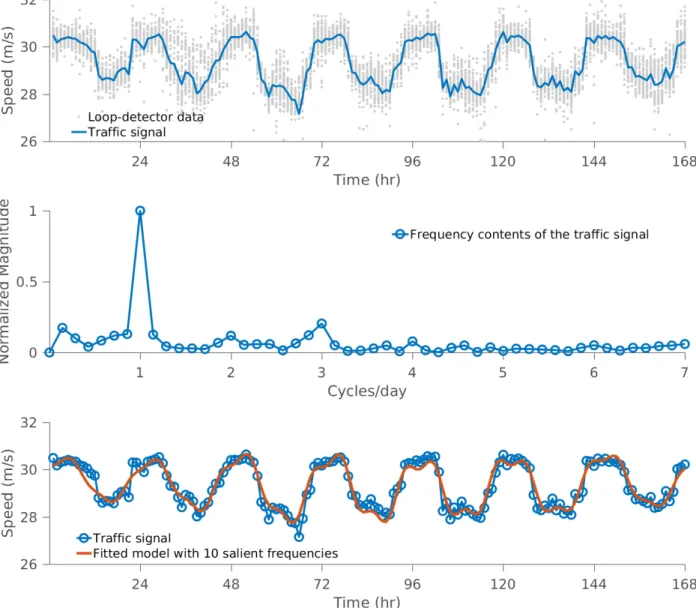
Traffic data can be scarce for certain time periods such as early-morning or late-night hours. In order to interpolate the data for these time periods, I exploit the fact that the traffic pattern is intrinsically periodic (as a result of periodic human behaviors). It thus has a sparse representation in the frequency domain. Based on this observation, I have developed a technique based on Compressed-Sensing (Donoho, 2006; Candes et al., 2006) to fill in missing travel time information and robustly recover the traffic pattern of a road segment over an entire traffic period (Li et al., 2017a). The details of this approach can be found in Chapter 2.
In order to test the effectiveness of my approach, I have adopted speed measurements from 38 loop detectors in the city of San Francisco. These data represent relatively complete and accurate measurements of traffic. The hourly average speed measurements of a single loop detector for a weekly period is termed the
Figure 1.4: Relative improvements measured in MSE of my technique over Lou et al. (Lou et al., 2009) on travel time. My technique outperforms Lou et al. (Lou et al., 2009) as the congestion level increases or as more GPS traces become available for the recovery task.
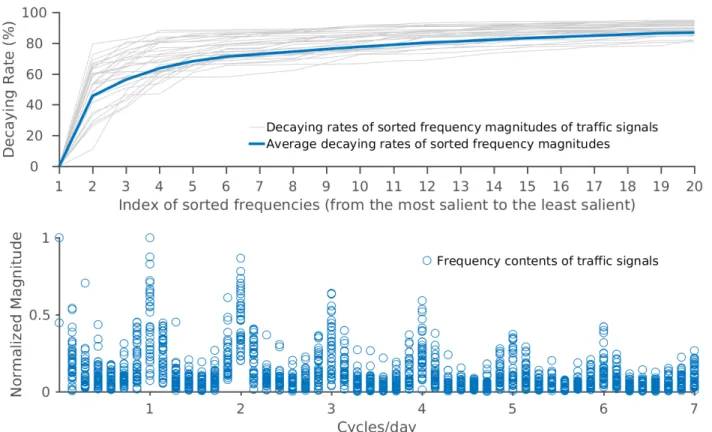
the 10 largest frequencies of the signal. These indicate that a traffic signal indeed has a sparse representation in the frequency domain, which is emphasized by the analysis of the decaying rates of frequency magnitude presented in the top panel of Figure 1.6.
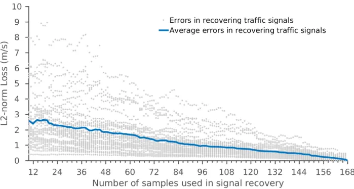
According to the Nyquist-Shannon Theorem, we need at least 168 measurements to fully recover a traffic signal, which are lacking as a result of the temporal sparsity of GPS data. However, Compressed Sensing promises that if a signal has a sparse representation and randomly distributed frequency components, we can have a accurate recovery of the signal. Those features do appear in a traffic signal as shown in Figure 1.6. This indicates that we can recover a traffic signal using Compressed Sensing. An example is shown in Figure 1.7. The robustness analysis of my approach can be found in Figure 1.8.
By confirming the applicability of Compressed Sensing algorithm to recovering traffic signals, we can proceed to apply it to real-world GPS datasets. To demonstrate that my approach can recover features of a traffic signal, I have adopted the metricfluidity∈[0,1](Hofleitner et al., 2012c), computed as the ratio of the estimated travel speed to the free-flow speed of a road segment. In Figure 1.9, I show the recovered traffic pattern using actual GPS data in San Francisco, which shows clear periodicity at one cycle per 24 hours.
Figure 1.7: A recovered traffic signal using my technique highly resembles its original form.
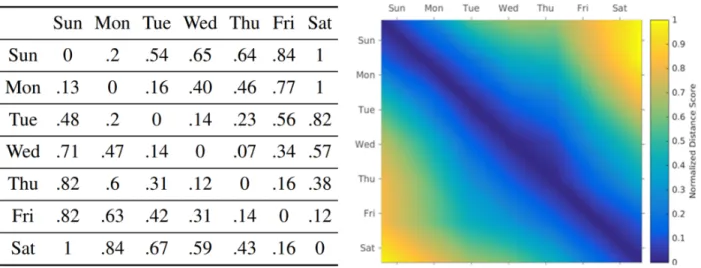
traffic conditions and the actual traffic conditions derived from the loop-detector data from San Francisco. The results are shown in Figure 1.10. The left panel shows the distance scores while the right panel shows the qualitative results: the upper triangle indicates the estimated quantities and the lower triangle indicates the actual quantities. The symmetrical pattern illustrates that my technique can produce accurate results compared to the ground-truth values.
1.3.1.3 Iterative Estimation and Spatial Missing Data Completion
While the deterministic approach introduced in the above section for estimating traffic conditions is efficient and effective, in order to further improve the accuracy for interpolating spatial missing data, I have developed an iterative algorithm that embedsmap-matchingandtravel-time estimationas its sub-routines (Li et al., 2018).
Figure 1.8: My technique shows robustness when the number of samples used in recovering a traffic signal decreases.
iteratively. Next, I proceed to establish baseline estimation of traffic conditions in areas without GPS data coverage using a nested optimization procedure (Yang et al., 1992) to ensure that certain traffic flow characteristics are met. The details can be found in Chapter 3.
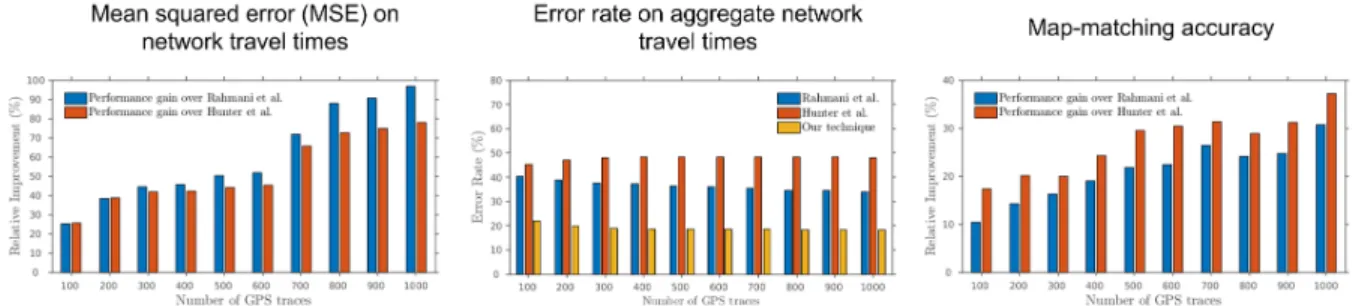
I have evaluated my approach using a real-world road network, which contains 5407 nodes and 1612 road segments. Additionally, 34 ground-truth travel times are established and over 10 million synthetic GPS traces are sampled based on the established heuristic travel times. I have compared my approach with two state-of-the-art methods, Hunter et al. (Hunter, 2014) and Rahmani et al. (Rahmani et al., 2015). The results show that my algorithm offers the lowest error rate and up to 97% relative improvement in estimation accuracy (see Figure 1.11).
Currently, most existing methods interpolate spatial missing measurements statically (Hellinga et al., 2008; Rahmani et al., 2015; Herring et al., 2010; Hunter, 2014; Tang et al., 2016b; Hunter, 2014; Li et al., 2017a). In order to account for the dynamic nature of traffic, I have leveraged traffic simulation for the interpolation task and developed an algorithm to guarantee the consistency of traffic flows on the boundaries of areas with and without GPS data (Li et al., 2017b).
Figure 1.9: Estimated traffic pattern of downtown San Francisco (TOP) and its spectral analysis (BOTTOM). The result from my technique demonstrates a clear daily trend, which is consistent with the periodic feature observed in loop-detector data from the same area.
Figure 1.11: My algorithm on map-matching and travel-time estimation achieves consistent improvements over the previous techniques (Rahmani et al., 2015; Hunter, 2014) in various measures.
traffic conditions in data-rich areas. This indicates we need to fine tune the simulation with the objective of enforcing minimal discrepancy between simulated traffic flows and previously estimated traffic flows. For this goal, I allow the simulation algorithm to alter “turning ratios” at intersections—parameters that determine how traffic will distribute itself to downstream road segments at an intersection. Using this design perspective, the objective then becomes deriving the optimal “turning ratios” such that the simulated traffic flows will respect the estimated traffic flows (from GPS data) at the boundaries that join data-deficient and data-rich regions.
The altered objective leads me to use simulation-based optimization for finding the optimal solution. However, as our goal is to reconstruct city-scale traffic, an optimization program at that scale could be computationally cost prohibitive. To remedy this issue, I have adopted a metamodel-based simulation optimization (Osorio et al., 2015). Compared to a stochastic microscopic traffic simulator, the metamodel is a deterministic function, thus is much more tractable and computationally efficient when running within an optimization routine. In order to make sure that the metamodel behaves similarly to the simulator, the metamodel is trained using simulations. This way we only need to run traffic simulation dozens of times (for training the metamodel) instead of hundreds or even thousands of times (for running simulation-based optimization).
Figure 1.12: The error level of my technique vs. simulation-only approach: For a given road network and a specific origin-destination demand, I first compute the differences between the two methods with respect to the ground truth. Then, I subtract these two differences to obtain one error difference measure (indicated by a gray cross). The mean, minimum, and maximum values of the average error level (indicated by the solid line) are respectively 7.8%, 0%, and 13%. In many cases, my technique even outperforms the simulation-only approach with much smaller differences to the ground truth, shown by the negative values.
Figure 1.13: The performance speedup of my technique over the simulation-only approach: my technique is
Figure 1.14: 2D traffic animation of regions in San Francisco: Northeast (top left), Central-East (top center), Central (top Right), Northwest (bottom). I have exaggerated the headlights and adopted an evening time period (i.e., Friday 7PM) to make vehicles more visible.
Figure 1.15: 3D traffic animation: a perspective overview (left), a topdown view (center), and a driver’s view (right).
After interpolating spatial missing data, I have fully reconstructed spatial-temporal traffic at the scale of a city. The reconstructed traffic can be visualized in many ways such as 2D flow map, 2D animation, and 3D animations. Some examples are shown in Figure 1.14, Figure 1.15, Figure 1.16, and Figure 1.17. These visual representations can be used to enable 1) analysis of traffic patterns at street level, region level, and the city level, and 2) virtual environment applications such as virtual tourism and the training of autonomous vehicles.
1.3.2 Autonomous Driving
Figure 1.16: Visualization of traffic patterns in San Francisco and Beijing. Four time periods of a week, namely Sunday 9AM, Tuesday 9AM, Thursday Noon, and Friday 7PM, are selected to illustrate weekend vs. weekday and morning vs. evening traffic. The traffic is measured by Volume Of Capacity (VOC). All computations are conducted in epoch time.
platform resides in a 3D virtual environment and is utilized to test a learned policy, simulate accidents, and generate labelled data. The second simulation platform operates in a 2D environment and serves as an “expert” to analyze and resolve an accident via planning alternative safe trajectories for a vehicle by considering its kinematic and dynamic constraints.
In addition, ADAPS represents a more efficient online learning mechanism compared to existing tech-niques such as DAGGER (Ross et al., 2011). The reason for the improvement is due to a switch from a “reset modeling” approach, in which we can only sample observations by putting an agent in its initial state distribution, to “generative modeling” approach, in which we can put an agent in an arbitrary state and sample observations by executing any action in that state. The reason that I can make this switch is because of two reasons: 1) the generation of training examples is from simulations that take vehicle kinematic and dynamic constraints into account, rather than merely executing a policy; 2) the assumption that we have access to all agent states in a simulation is because the simulation is conducted in retrospect of an accident, thus viable.
In order to understand the theoretical results, I will briefly introduce the notation and definitions used in the analysis. The problem we consider is aT-step control task. Given the observationφ=φ(s)of a states at each stept∈[[1, T]], the goal of a learner is to find a policyπ∈Πsuch that its produced actiona=π(φ) will lead to the minimal cost:
ˆ
π = arg min π∈Π
T X
t=1
C(st, at), (1.1)
whereC(s, a)is the expected immediate cost of performingains. For many tasks such as driving, we may not know the true value ofC. Instead, the observed surrogate lossl(φ, π, a∗)is commonly minimized. This loss is assumed to upper boundC, based on the approximation of the learner’s actiona=π(φ)to the expert’s actiona∗=π∗(φ). I denote the distribution of observations attasdtπ, which is the result of executingπfrom timestep1tot−1. Consequently,dπ = T1 PTt=1dtπ is the average distribution of observations by executing π forT steps. The goal of solving an SPC task is to obtainˆπ—a policy that can minimize the observed surrogate loss under its own induced observations with respect to an expert’s actions for those observations:
ˆ
π= arg min π∈Π
Eφ∼dπ,a∗∼π∗(φ)[l(φ, π, a
∗
)]. (1.2)
I further denote=Eφ∼dπ∗,a∗∼π∗(φ)[l(φ, π, a
∗)]as the expected loss under the training distribution induced
By simply treating expert demonstrations as i.i.d. samples, the discrepancy betweenJ(ˆπ)andJ(π∗) isO(T2)(Syed and Schapire, 2010; Ross et al., 2011). Given the error of a typical supervised learning is
O(T ), this demonstrates the additional cost due to covariate shift when solving an SPC task via standard supervised learning.
DAGGER (Ross et al., 2011) has been used to solve an SPC task by keeping theO(T )error. To illustrate its result, I introduce more definitions: the best policy at theith iteration (trained using all observations from the previousi−1iterations) is denoted asπi; for any policyπ ∈ Π, we have its expected loss under the observation distribution induced byπiasli(π) =Eφ∼dπi,a∗∼π∗(φ)[li(φ, π, a∗)], li ∈[0, lmax]; the minimal loss in hindsight afterN ≥iiterations is denoted asmin = minπ∈ΠN1 PNi=1li(π)(i.e., the training loss afterN iterations); the average regret isregret = N1
PN
i=1li(πi)−min. Then, the accumulated error after T-step using DAGGER (Ross et al., 2011) is bounded by the summation of three terms:
J(ˆπ)≤T min+T regret+O(f(T, lmax)
N ), (1.3)
where f(·) is the function of fixedT andlmax. The second term tends to 0 if a no-regret algorithm is used (Hazan et al., 2007). The third term tends to0ifN → ∞.
1.3.2.1 Theoretical Results
With the above-introduced background, I can introduce the following theoretical results.
Theorem 1.1. If the surrogate losslupper bounds the true costC, by collectingKtrajectories using ADAPS at each iteration, with probability at least1−µ,µ∈(0,1), ADAPS offers the following guarantee:
J(ˆπ)≤J(¯π)≤Tˆmin+Tˆregret+O
T lmax s
logµ1 KN
ADAPS uses principled simulations for generating them. With these changes, this theorem can lead to the following Corollary.
Corollary 1. Iflis convex inπfor anysand it upper boundsC, and Follow-the-Leader is used to select the learned policy, then for any >0, after collectingO
T2l2
maxlog1µ
2
training examples, with probability at least1−µ,µ∈(0,1), ADAPS offers the following guarantee:
J(ˆπ)≤J(¯π)≤Tˆmin+O()
Now, we only need the training error ˆmin to be minimal, which is achievable via standard supervised learning.
1.3.2.2 Experimental Results
I have tested my method empirically in three simulated scenarios, namely a straight road (representing a linear geometry), a curved road (representing a non-linear geometry), and an open ground. The straight and curved roads represent anon-roadscenarios with a static obstacle in the form of a traffic cone. The open ground represents anoff-roadscenario with a dynamic obstacle in the form a vehicle.
I have compared my policy to the technique from Bojarski et al. (Bojarski et al., 2016), as it is one of the representative approaches for end-to-end autonomous driving. Usually, this type of approach is limited to single-lane following (Chen et al., 2015; Xu et al., 2017; Zhang and Cho, 2017; Codevilla et al., 2017) or
off-roadcollision avoidance (LeCun et al., 2005) behaviors.
For the two on-road scenarios, I collect training datasets fromstraight road with or without an obstacle
andcurved road with or without an obstacle. This separation enables six policies for testing the effectiveness oflearning from accidents:
• My policy: trained with just the lane-following dataOf ollow;Of ollowadditionally trained after analyzing an accident on the straight roadOstraight; andOstraightadditionally trained after analyzing an accident on the curved roadOf ull.
• Similarly, for the policy from Bojarski et al. (Bojarski et al., 2016):Bf ollow,Bstraight, andBf ull.
showing both policies can finish all 50 laps safely. Then, I add an obstacle to the straight road and test both policies again. Since both policies have not trained on the accident data yet, they both run into the obstacle and cause an accident.
After analyzing the occurred accident and incorporating the accident data into training, I obtain two new policiesOstraightandBstraight. As expected,Ostraightavoids the obstacle, whileBstraightcontinues to cause collision.
I proceed to add an obstacle to the curved road, after a similar process, I obtainOf ull andBf ull. Again, as expected,Of ull manages to perform both lane-following and collision avoidance behaviors. Bf ull, in contrast, leads the vehicle to an accident. These two cases are illustrated in Figure 1.18 LEFT and CENTER.
Figure 1.18: LEFT and CENTER: the comparisons between my policyOf ull(TOP) and Bojarski et al. (Bo-jarski et al., 2016),Bf ull(BOTTOM).Bf ullcauses collision whileOf ullsteers the AV away from the obstacle. RIGHT: the accident analysis results on the open ground. I show the accident caused by an adversary vehicle (TOP); then I show, after additional training, the AV can avoid the adversary vehicle (BOTTOM).
In order to test the generalization of my policy, I uniformly sampled 50 positions to place the obstacle on a3meters line segment that is perpendicular to the direction of a road and in the same lane as the vehicle. The success rate (i.e., avoid an obstacle and resume normal driving) are documented in Table 1.2.
Test Policy and Success Rate (out of 50 runs)
Scenario Bf ollow Of ollow Bstraight Ostraight Bf ull Of ull
Straight road / Curved road 100% 100% 100% 100% 100% 100%
Straight road + Static obstacle 0% 0% 0% 100% 0% 100%
Curved road + Static obstacle 0% 0% 0% 0% 0% 100%
Table 1.2: Test Results of On-Road Scenarios: my policiesOstraight&Of ull can lead to robust collision avoidance and lane-following behaviors.
policy can steer the vehicle away from the adversary vehicle and resume its direction to the target. This is illustrated in Figure 1.18 RIGHT.
The key to rapid improvements of a policy is the generation of sufficient and heterogeneous training data. In Figure 1.19, I show the visualization results of images collected via my method and DAGGER (Ross et al., 2011) in one learning iteration. By progressively increasing the number of sampled trajectories, my method results in much more heterogeneous training data, which, when produced in a large quantity, can greatly facilitate the update of a policy.
1.4 Thesis Statement
My thesis statement is as follows:
Urban mobility can benefit from better designed intelligent transportation systems which can be further
improved with 1) accurate and efficient reconstruction of city-scale traffic at the macroscopic level and 2)
enhanced control and learning mechanisms for individual vehicles at the microscopic level.
To support this thesis, at the macroscopic level, I have developed methods to efficiently estimate traffic conditions, accurately interpolate spatial-temporal missing traffic data, dynamically reconstruct traffic flows, and produce visual analytics in various forms. At the microscopic level, I have developed a framework to simulate and analyze various driving scenarios while automatically producing labeled training data, which, when combined with an efficient online learning mechanism and an effective policy architecture, can lead to robust control policies for autonomous driving.
1.5 Organization
CHAPTER 2: CITYWIDE ESTIMATION OF TRAFFIC DYNAMICS VIA SPARSE GPS TRACES
2.1 Introduction
Traffic is ubiquitous in modern cities, impacting their social, economic, and environmental developments. However, ever-present gridlock and congestion keep challenging transportation researchers and urban planners. According to the 2015 Urban Mobility Scorecard (Schrank et al., 2015), traffic congestion causes an extra 6.9 billion travel hours and 3.1 billion gallons of fuel consumption annually in the United States, which costs are approximately $160 billion. As an increasing number of metropolitan areas experience severe traffic conditions and the overall cost is estimated more than one trillion U.S. dollars worldwide, the ability to analyze and understand traffic dynamics is becoming crucial.
In order to understand traffic congestion, first, we need to obtain its measurements. Traditionally, traffic measurements are collected via in-road sensors such as loop detectors and video cameras (Leduc, 2008). While these sensors produce relatively accurate records, the high expenditures for installation and maintenance prevent them from being deployed over an entire city, rather than major roads and highways. Consequently, the lack of sensing infrastructure for arterial streets—which comprise the majority of a city—has made the large-scale traffic measuring task difficult.
Mobile data such as GPS traces, in contrast, are more promising sources for understanding citywide traffic dynamics due to their much boarder coverage. However, such data are limited in two aspects: 1) inevitable errors in measurement and transmission often yield reported locations off the road, and 2) due to energy and privacy concerns, GPS data commonly have alow sampling rate, meaning that the time difference between consecutive points can be large (e.g., greater than 60 seconds), and alow penetration rate, meaning that only a small percentage of traffic population is willing to send location reports.
accurately estimated. Because of thelow sampling rate, the inferred path between two consecutive GPS points is likely to consist of multiple road segments, but only the aggregate travel time (i.e., the difference between the GPS timestamps) is known. The aggregate travel time needs to be distributed to individual road segments, which process is namedtravel time allocation. Third, in order to understand the full traffic dynamics of a city, traffic data are needed for an entire traffic period for each road segment of a city’s road network. However, GPS data often do not provide complete temporal coverage as they are commonly scarce in late night and early morning hours. The process for interpolating the missing temporal information is namedmissing value completion.
Many efforts have been made towards improving the effectiveness of the abovementioned three processing steps. To be specific, the low sampling rate introduces issues: two consecutive GPS points are likely far apart from each other and multiple paths can exist for connecting them (especially in a complex urban environment). Thus, inferring the true traversed path between them is challenging. Many state-of-the-artmap-matching
approaches use the shortest-distance criterion (Lou et al., 2009; Yuan et al., 2010; Miwa et al., 2012; Hunter et al., 2014; Chen et al., 2014; Quddus and Washington, 2015) to infer the traversed path. While this criterion is viable when a road network is under or close to a free-flow condition, it can introduce errors in a congested environment where other paths (not the shortest-distance path) can be traveled with less time and will be preferred by GPS devices and most drivers. If we have a wrongly inferred path, the timestamp difference (i.e., aggregate travel time) will be distributed to a wrong set of road segments. In other words, the introduced errors will be carried over to the subsequent steptravel time allocation, causing the overall estimation of traffic conditions deteriorated.
Figure 2.1: Pipeline of my framework. Map Matching and Travel Time Allocation are applied on individual time intervals, while Missing Value Completion is performed over all time intervals.
on Compressed Sensing (Donoho, 2006; Candes et al., 2006) to interpolate missing travel information over an entire traffic period. The overview of my framework pipeline is shown in Figure 2.1.
I have extensively evaluated and tested the effectiveness of my approach and compared it to the method developed by Lou et al. (Lou et al., 2009), using GIS data from a synthetic road network and the city of San Francisco (Piorkowski et al., 2009). The results demonstrate major improvements over the existing method (Lou et al., 2009) in various steps during the estimation process. In summary, the contributions of this work are the following:
• A novel perspective (switching from the shortest-distance criterion to the shortest travel-time criterion) in addressing sparse GPS traces during map-matching;
• An improved travel time allocation technique which incorporates estimated intermediate traffic conditions into computation;
• An efficient and robust method for interpolating missing traffic measurements in traffic patterns.
2.2 Related Work
Over the last few decades, the estimation of traffic conditions has gained increasing scholarly atten-tion (Celikoglu, 2007; Celikoglu et al., 2009; Gao, 2012; Abadi et al., 2015; Kachroo and Sastry, 2016; Agarwal et al., 2016). Early studies on traffic estimation have focused on traffic states on highways using accurate measurements from stationary sensors such as loop detectors and video cameras (Leduc, 2008). Recent advancements have shifted to combining multiple data sources and traffic simulation models for achieving better estimation results (Work et al., 2010; Sun and Work, 2014; Gning et al., 2011; Li et al., 2014; Celikoglu and Silgu, 2016; Hajiahmadi et al., 2016). However, the scenarios of interest in these studies were limited to road segments with lengths of a few kilometers.
The increasing availability of GPS data provides new means for conducting large-scale estimation of traffic conditions. However, as GPS data are inherently noisy, the estimated traffic conditions usually do not satisfy the flow conservation requirement assumed by many simulation models (Phan and Ferrie, 2011; Kong et al., 2013; Zhang et al., 2013). As a result, new studies that consist of several steps for the estimation task, are emerging.
The first step,map-matchingaddresses the problem of mapping off-the-road GPS points onto a road network and identifies the true traversed path between consecutive GPS points. However, GPS data could contain alow sampling rate, which causes points to be far away from each other and making the selection among multiple paths connecting the points difficult. In order to determine the “actual” traversed path of a vehicle, a common approach is to use the shortest-distance criterion to connect two GPS points on a road network (Lou et al., 2009; Yuan et al., 2010; Miwa et al., 2012; Hunter et al., 2014; Chen et al., 2014; Quddus and Washington, 2015). Nonetheless, the shortest-distance assumption can lead to errors in a congested environment, in which alternative paths can be traveled faster than the shortest-distance path and preferred by GPS devices and drivers. Essentially, the shortest-distance criterion only uses spatial information (i.e., longitude and latitude of GPS points, and the geometry of a road network), while ignoring the temporal information (i.e., timestamps) recorded in GPS reports. This happens primarily due to the travel times of a road network are largely unknown, causing the temporal information has nothing to be compared with (Tang et al., 2016a; Rahmani and Koutsopoulos, 2013).
times of road segments using intuitive and empirical observations of traffic patterns in real life. Rahmani et al. (Rahmani et al., 2015) take a non-parametric approach, performing an estimation using a kernel-based method. Probabilistic frameworks have also been developed to conduct an estimation of traffic conditions (Khosravi et al., 2011; Westgate et al., 2013; Herring et al., 2010; Hofleitner et al., 2012a; Kuhi et al., 2015). While significant improvements have been achieved, these methods all perform the estimation steps sequentially, causing the limitations ofmap-matchingwill be carried over to its subsequent steps and eventually deteriorate the overall estimation accuracy.
Researchers have also proposed solutions to missing value completion. For example, tensor-based approaches (Wang et al., 2014a; Asif et al., 2016), which explore correlations among nearby road segments, have been developed. From Zhu et al. (Zhu et al., 2013) and Mitrovic et al. (Mitrovic et al., 2015), algorithms based on Compressed Sensing have been proposed by taking an entire road network as the study subject. Interpolating missing values has also been addressed in an online setting (Anava et al., 2015). Nevertheless, the abovementioned methods were not designed to tackle the problem of estimatingfulltraffic dynamics of individual road segments over an entire city—a subject for which little progress has been made (Hofleitner et al., 2012c).
2.3 Traffic Velocity Field Reconstruction
I take a holistic view of map-matching and travel time allocation, and propose a noval method to reconstruct the velocity field of a road network. Starting with some definitions in this section, I then discuss methodologies and implementation details of my approach. My algorithm is evaluated and validated using a synthetic road network with microscopic traffic simulation.
2.3.1 Notation and Definitions
Aroad networkis defined as a directed graphG= (V, E)in which edgesEdenote road segments and nodesV represent intersections and terminal points. Each road segmente∈Econtains several attributes: the lengthe.len, the maximum/free-flow travel speede.vmax, the minimum/free-flow travel timee.tmin = e.ve.len
max,
and the maximum/jam densitye.kmax.
Apathfrom nodegto nodehon a networkg p his a collection of road segmentsp={e1, e2, . . . , en},
Figure 2.2: An example illustrating a failure using the shortest distance criterion for map-matching trace StoT1,T2, orT3. LEFT: By matching travel time of traceSand road conditions, the correct pathT1is identified. RIGHT: By only considering the shortest distance path,Sis mismatched toT3.
S ={s1, s2, . . . , sn}in which each point is a tuplesi =< si.x, si.y, si.t >containing longitude, latitude,
and a timestamp.
2.3.2 Velocity Field Estimation
Given the periodicity of traffic patterns over a week (Hofleitner et al., 2012c), I study traffic dynamics over the region of interest in a weekly period. I discretize one week into hourly time intervals and assume that traffic conditions remain the same within one hour on a road segment. For simplicity, I restrict my discussion of estimating the velocity field to one time interval (i.e., one hour). The process can be trivially extended to cover other time intervals of an entire traffic period.
Ideally, if the actual traversed path of a vehicle is known and the generated GPS points are exactly on the road, I can derive the average travel speed of a path p that connects GPS points si andsi+1 as
p.t =
P e∈pe.len
si+1.t−si.t. However, GPS points are often off-the-road due to inherent measurement and sensing
errors, and the underlying path of a vehicle is also unknown. To address these issues, a number of candidate nodes of the network are considered for mapping a GPS point, based on their distances to the point. Then, one of the paths connecting a pair of candidate nodes of two consecutive GPS points is selected to represent the actual path. As mentioned earlier, one common approach for choosing such a path is taking the shortest distance criterion (Lou et al., 2009; Yuan et al., 2010; Miwa et al., 2012; Hunter et al., 2014; Chen et al., 2014; Quddus and Washington, 2015), which can produce errors in a congested environment (an illustrative example is shown in Figure 2.2).