STATISTICAL TOOLS FOR GENERAL ASSOCIATION TESTING AND CONTROL OF FALSE DISCOVERIES IN GROUP TESTING
Pratyaydipta Rudra
A dissertation submitted to the faculty at the University of North Carolina at Chapel Hill in partial fulfillment of the requirements for the degree of Doctor of Philosophy in
the Department of Biostatistics in the Gillings School of Global Public Health.
Chapel Hill 2015
Approved by:
Fred A. Wright Andrew Nobel Wei Sun Yun Li
c
ABSTRACT
Pratyaydipta Rudra: Statistical Tools for General Association Testing and Control of False Discoveries in Group Testing
(Under the direction of Fred A. Wright and Andrew Nobel)
In modern applications of high-throughput technologies, it is important to identify pairwise associations between variables, and desirable to use methods that are powerful and sensitive to a variety of association relationships. In the first part of the disser-tation, we describe RankCover, a new non-parametric association test for association between two variables that measures the concentration of paired ranked points. Here ‘concentration’ is quantified using a disk-covering statistic that is similar to those em-ployed in spatial data analysis. Analysis of simulated datasets demonstrates that the method is robust and often powerful in comparison to competing general association tests. We also illustrate RankCover in the analysis of several real datasets. Using RankCover, we also propose a method of testing the association of two variables while controlling the effect of a third variable.
anno-tated to the gene corresponding to individual hypotheses. Heterogeneity of effect sizes in different groups is considered by the introduction of a random effects component. Our method, entitledRandom Effects model and testing procedure for Group-level FDR control(REG-FDR) assumes a model for alternative hypotheses for the eQTL data and controls the FDR by adaptive thresholding.
ACKNOWLEDGEMENTS
I wish to express my sincerest gratitude to my advisor Dr. Fred Wright for guiding and mentoring me. I have profoundly benefited from his guidance over the past five years. His enthusiasm for pursuing interesting statistical problems at the highest level of scientific integrity and rigor has been a constant source of inspiration for my research. I deeply thank him for allowing me the space to think myself and for fostering my capacity as an independent researcher. I feel very fortunate to have him as my advisor and the lessons that I learnt through this journey will always stay with me.
I would like to thank my co-advisor Dr. Andrew Nobel for his support and critical remarks on my work. His constant invigilation and assistance helped me a lot.
I would also like to thank all the other members in my thesis committee, namely, Drs Wei Sun, Yun Li and Karen Mohlke, for careful review and providing valuable suggestions in improving the contents of this thesis.
I am extremely thankful and indebted to Dr. Pranab Kumar Sen for providing support whenever I needed. I thank Dr. and Mrs. Sen also for sponsoring the Kalyani Sen International Student Scholarship in Biostatistics that helped me to overcome the financial burden of studying in a foreign country.
I sincerely thank my friend Sayan Dasgupta for his academic and non-academic guidance throughout the past five years.
I am fortunate enough to be surrounded by a wonderful set of friends, who de-serves special mention. Sujatro Chakladar, Lopamudra Kundu, Anjishnu Banerjee, Wangsuk Choi, Suprateek Kundu, Swarnava Mukherjee, Ranajoy Bhattacharjee, An-abil Gayen, Vivek Atal, Anjan Mandal, Rakesh Krishnan Poduval, Avijit Shee, Projjwal Das, Jishnu Datta - they all were beside me any time I needed.
I have been blessed to be friends with Gen Li, Sayantan Banerjee, Abhishek Pal Majumder, Subhamay Saha and Pourab Roy, the academic discussions with whom highly enriched me.
I would like to thank my parents for their faith in me and allowing me to be as ambitious as I wanted. It was under their watchful eye that I gained so much drive and an ability to tackle challenges in life. I would not be here without their sacrifices, patience, continuous support and unconditional love.
Last but not the least, I express my heartiest thanks to my wife Sreemala Das Majumder, who has provided immense support in tough times. Without her constant encouragement and love, this journey would not have been possible. Even after remain-ing thousands of miles away, she has always tried her best to provide me company and support.
TABLE OF CONTENTS
LIST OF TABLES . . . xi
LIST OF FIGURES. . . xii
CHAPTER 1 : INTRODUCTION . . . 1
1.1 Testing of General Association . . . 1
1.1.1 Classical non-parametric tests . . . 2
1.1.2 Methods in spatial statistics . . . 2
1.1.3 Other methods of detecting general association . . . 4
1.1.4 Recent advancements . . . 5
1.1.5 Summary . . . 7
1.2 Control of False Discovery Rate for Grouped Hypotheses . . . 7
1.2.1 Classical methods and family-wise error rate . . . 8
1.2.2 The false discovery rate approach . . . 9
1.2.3 Extension and different approaches to FDR . . . 10
1.2.4 The empirical Bayes approach and local false dis-covery rate . . . 12
1.2.5 Grouped Hypotheses . . . 13
1.2.6 Application in eQTL studies . . . 15
1.2.7 Summary . . . 15
1.3 Overview of the thesis . . . 16
CHAPTER 2 : A PROCEDURE TO DETECT GENERAL ASSOCIATION . . . 17
2.2 The test statistic . . . 18
2.3 Choice of parameters and distance metric . . . 22
2.4 Fast Computation of the test statistic . . . 26
2.5 Exact expectation of the RankCover statistic for Man-hattan distance . . . 27
2.6 Large sample properties of RankCover . . . 30
2.6.1 Coverage Process . . . 30
2.6.2 Asymptotic Negligibility of the edge effect . . . 31
2.6.3 Asymptotics of coverage for Boolean process . . . 32
2.6.4 Applicability of the results toRankCover . . . 33
2.7 Simulation Results . . . 35
2.7.1 Comparison of different methods for simulated datasets . . . 35
2.7.2 Comparison of dCor and Rank Correlation . . . 40
2.8 Application on Real Data . . . 40
2.8.1 Example 1: Eckerle4 data . . . 40
2.8.2 Example 2: Aircraft data . . . 41
2.8.3 Example 3: ENSO data . . . 42
2.8.4 Example 4: Yeast data . . . 43
2.9 Method to test the association of two variables after adjusting the effect of a third variable . . . 45
2.10 Discussion and future work . . . 49
CHAPTER 3 : CONTROL OF FALSE DISCOVERIES IN GROUPED HYPOTHESIS TESTING FOR EQTL DATA . . . 51
3.1 Structure of the eQTL data and the hypotheses . . . 51
3.2 The empirical Bayes set up . . . 52
3.4 An EM algorithm to estimate REG-FDR parameters . . . 55
3.5 The Z-REG-FDR model . . . 57
3.6 Results of Z-REG-FDR as an approximate maximum likelihood estimation . . . 64
3.7 Comparison with other methods . . . 68
3.8 Advantage of Z-REG-FDR over other methods . . . 71
3.9 Effect of more than one causal SNPs . . . 72
3.10 Analysis of real data . . . 73
3.11 Inverse Average Method . . . 74
3.12 Discussion and future work . . . 78
CHAPTER 4 : MULTI-TISSUE EXTENSION OF Z-REG-FDR . . . 81
4.1 Data, notations and basic assumptions . . . 81
4.2 Further assumptions and the MT-Z-REG-FDR model . . . 82
4.3 The likelihood . . . 84
4.4 Application on simulated datasets . . . 85
4.5 Application on real datasets . . . 86
4.6 Discussion and future work . . . 86
APPENDIX A: TECHNICAL DETAILS FOR CHAPTER 2 . . . 88
A.1 Details of the analysis of simulated data . . . 88
A.2 Details of Simulation results for different marginal dis-tributions of the variables . . . 89
A.3 Details of real data analyses . . . 91
A.3.1 Example 1: Eckerle4 data . . . 91
A.3.2 Example 2: Aircraft data . . . 91
A.3.3 Example 3: ENSO data . . . 92
APPENDIX B: TABLES OF THRESHOLDS OF RANKCOVER . . . 93
APPENDIX C: TECHNICAL DETAILS FOR CHAPTER 3 . . . 107
C.1 Pre-processing of the GTEx data . . . 107
C.2 Details of the simulation procedures for Z-REG-FDR . . . 108
C.3 Details of the simulation procedures for two causal SNPs . . . 108
C.4 Details of the simulation procedures for inverse average . . . 109
LIST OF TABLES
Table 1.1 Showing the cross-classification of true and false null
hypothesis against the decision to accept or reject . . . 9
Table 3.1 Showing summary of the simulation studies with di-rectly simulated z from an AR(1) model with correlation
ρ . . . 59 Table 3.2 Showing summary of the simulation studies using the
SNP matrix from real data . . . 65 Table 3.3 Showing summary of the simulation studies where
the SNP matrix has an AR(1) structure with correlation ρ . . . 66 Table 3.4 Showing summary of the simulation studies for two
causal SNPs . . . 72 Table 3.5 ShowingZ-REG-FDRparameter estimates and
sum-mary of the findings for the GTEx datasets . . . 73
Table 4.1 Showing the mean power of the different methods for the nine cases. eg. Beta-Normal refers to the case where
LIST OF FIGURES
Figure 1.1 Illustration of paired adjusted distances underlying dCor. (top row) Illustration of dCor for a quadratic rela-tionship between x and y.(bottom row) A circular relation-ship between x and y. The adjusted paired distances show
little correlation. . . 6
Figure 2.1 Illustration of RankCover for sample size n = 50: A.Scatter plot of the two variables. B. Scatter plot on the rank scale C. Disks laid on the scatter plot on rank scale using Euclidean distance D. Disks laid on the scatter plot
on rank scale using Manhattan distance. . . 18 Figure 2.2 Showing the Grid based approach of RankCover . . . 19 Figure 2.3 Showing the comparison of power of the method
using the area under the EDF (AUC method) and that of the method using δopt =
√
n . . . 21 Figure 2.4 Showing the expected δ for which A.T(D1) = 1 B.
ˆ
FRG(D1) = 1 . . . 22 Figure 2.5 Showing the mean, sd and coefficient of variation of
T(δ) for sample size 50 (Euclidean distance is used) . . . 23 Figure 2.6 Showing the mean, sd and coefficient of variation of
T(δ) for sample size 100 (Euclidean distance is used) . . . 24 Figure 2.7 Showing the δ for which standard deviation ofT(δ)
is minimum for different sample sizes . . . 25 Figure 2.8 Showing the Average p-value using different disk
sizes when testing against various forms of association . . . 25 Figure 2.9 Showing the pre-computed thresholds for theRankCover
method with Manhattan distance. 100000 simulations were used to calculate the thresholds in each case. Simulations were performed for n= 20, ...,100. For large values ofn, to reduce computation, tables were generated by (i) perform-ing direct simulation for the values of n at, and just prior to, the jump points, followed by (ii) linear interpolation for
Figure 2.11 Schematic to illustrate calculation of P(Iij = 1) for
1≤i≤n,1≤j ≤n. . . 27 Figure 2.12 Showing the existence of (i0, j0) for a point (i, j)
outside the n×n region . . . 29 Figure 2.13 Showing the difference in mean and standard
devia-tion between total coverage C for Boolean process and the
RankCover statistic. . . 33 Figure 2.14 Showing the√ A.mean and B. standard deviation of
n(C−E(C)) for Boolean process and the corresponding
statistic for ˆFRG(δ). . . 34
Figure 2.15 Showing the√ A.mean and B. standard deviation of n(C−E(C)) for Boolean process and the corresponding
statistic for T(δ). . . 35 Figure 2.16 Showing the scatter plots for different relationships
between the pair of variables (low noise level). . . 36 Figure 2.17 Showing the power of different methods (type-Iα=
0.05) against different relationships at varying noise levels
(Manhattan distance), n = 50. . . 37 Figure 2.18 Showing the power of different methods (type-Iα=
0.05) against different relationships at varying noise levels
(Euclidean distance), n = 50. . . 38 Figure 2.19 Showing the power comparison of dCor and
Spear-man’s rank correlation . . . 39 Figure 2.20 Showing the scatter plot and the fitted curve for the
Eckerle4 dataset . . . 41 Figure 2.21 Showing the scatter plot and the density estimate
contours for the aircraft speed and wing span . . . 42 Figure 2.22 Showing the scatter plot and the fitted curve for the
Figure 2.23 A. The plot comparing the FDR adjusted q-values of the test using RankCover and that using dCor for the genes in Spellman’s list in a log scale. It is evident that most of the genes in Spellman’s list have a smaller q-value when the RankCover test is used. B. A similar plot com-paring the q-values of RankCover and MIC. C. A similar plot comparing the q-values ofRankCover and HHG. D-I. Examples of genes in the Spellman’s list that were identi-fied by RankCover, but not by at least one of dCor, MIC or HHG. The values in parentheses are the Spellman scores
for the genes. . . 44 Figure 2.24 Showing the effect of number of strata on the type-I
error of stratified approach. The horizontal line is the type-I error of the RankCover test in the ideal situation where one knows the exact form of x-z and y-z dependence. A.
x-z and y-z are linear B. x-z is linear and y-z is quadratic. . . 47 Figure 2.25 Showing the effect of number of strata on the power
of stratified approach. The horizontal line is the power of the RankCover test in the ideal situation where one knows the exact form of x-z and y-z dependence. A.x-y, x-z and y-z are linear, all the slopes have the same sign B. x-y is quadratic,x-z and y-z are linearC. x-yis circular, x-z and y-z are linear D. x-y is circular, x-z is linear and y-z is quadratic E. x-y is X14, x-z is linear and y-z is quadratic
F. x-z and y-z are linear with positive slopes, x-y is linear
with a negative slope. . . 48
Figure 3.1 Comparing the elements of conditional covariance matrix ofZ under the null and those under the alternative. TheR2as well as the maximum difference in the conditional means are reported. The correlation structure of the SNPs
is assumed to be AR(1). β is the effect size. . . 64 Figure 3.2 Comparing the elements of conditional covariance
matrix ofZ under the null and those under the alternative. TheR2as well as the maximum difference in the conditional means are reported. The correlation structure of the SNPs
is obtained from a real data. β is the effect size. . . 64 Figure 3.3 Showing the comparison of the estimates using
REG-FDR and Z-REG-REG-FDR. Except a small number of cases, the two estimates agree with each other. The blue lines show
Figure 3.4 Showing the A. estimated lfdr and B. estimated
FDR for REG-FDRand Z-REG-FDR. . . 67 Figure 3.5 Showing the histograms of correlations between the
estimated FDR based on the true values of the parameters
and that based on A.REG-FDR B. Z-REG-FDR. . . 68 Figure 3.6 ShowingA.the surface plot andB.the contour plot
of expected pseudo-log-likelihood surface for the
Z-REG-FDR method. True π0 and σ are 0.2 and 3 respectively. . . 69 Figure 3.7 Showing the power curves of different methods for
varying combinations of the true parameter values. . . 69 Figure 3.8 Showing the histogram of correlations between
esti-mated FDR using the permutation method and that using
Z-REG-FDR. . . 70 Figure 3.9 Showing the histogram of correlations between
esti-mated FDR using the true parameter values and that using
permutation method or Bonferroni method. . . 71 Figure 3.10 Showing the sharpness of the Inverse Average bound
using a simulated data. The black line shows the sorted true gene lfdr’s and the red dots are the inverse average of the corresponding gene-SNP level lfdr’s. The simulation
procedure used is similar to the scheme described in Section 3.5. . . 75 Figure 3.11 Showing the sharpness of the Inverse Average bound
after adjustment. The black line shows the sorted true gene lfdr’s and the red dots are the adjusted inverse average of
the corresponding gene-SNP level lfdr’s. . . 76 Figure 3.12 Showing the sharpness of the Inverse Average bound
for a blocked data structure. The black line shows the sorted true gene lfdr’s and the red dots are the adjusted inverse average for the hypothesis of causality. The blue dots are the adjusted inverse average for the gene-SNP level
significance test. . . 77 Figure 3.13 Showing the sharpness of the Inverse Average bound
for a window type data structure. The black line shows the sorted true gene lfdr’s and the red dots are the adjusted inverse average for the hypothesis of causality. The blue dots are the adjusted inverse average for the gene-SNP level
Figure 3.14 Showing the comparison of inverse average method
CHAPTER 1: INTRODUCTION
1.1 Testing of General Association
The need for statistical methods to identify general pairwise association measured between variables is increasingly recognized, as evidenced by recent attention to meth-ods such as distance correlation (dCor) (Sz´ekely et al. 2007, Sz´ekely and Rizzo 2009), Maximal Information Coefficient (MIC) (Reshef et al. 2011), and the Heller-Heller-Gorfine (HHG) method (Heller et al. 2013). The term general association refers to any departure from independence among random variables, and methods differ in the types of departures to which they are sensitive. The need for general association tests is perhaps greatest for analysis of large datasets, for which discovery-based approaches are needed, without prior hypotheses regarding the form or structure of dependence. In addition to the need to test dependence among pairs of variables as a primary analysis, dependencies can invalidate inference for downstream methods that require independence among input variables (Albert et al. 2001).
1.1.1 Classical non-parametric tests
Classical tests attempting to detect general association date back to the early part of the last century with Spearman’s rank correlation (Spearman 1904) and Kendall’s tau (Kendall 1938). Standard tests based on these rank correlations assume values are not tied, and are primarily designed for monotone relationships, but are not principally different in spirit from Pearson’s product moment correlation.
Many trend tests (Mann 1945, Kendall 1975, Cuzick 1985, Hamed and Ramachan-dra Rao 1998) were devised over the years for testing linear and non-linear trends, pri-marily in time series data. However, they also suffer from insensivity to non-monotone relationships.
1.1.2 Methods in spatial statistics
The spatial statistics literature is abundant with tests of complete spatial random-ness (CSR), which is closely related to the general association of two variables. Com-plete spatial randomness as defined by Diggle (1983) occurs when
1. the number of events in any planar region A with area |A| follows a Poisson distribution with meanλ|A|.
2. given n events xi in a region A, the xi’s form an independent random sample
from the uniform distribution onA.
of other points in the neighborhood of it, but the alternative of inhibition is not very relevant for testing general association. These differences can be somewhat reduced by using the ranks of the two variables while testing general association, since each component of rank(X) and rank(Y) has a discrete uniform distribution for any two jointly distributed random variables X and Y. However, note that these components are not independent since a rank vector needs to be a permutation of (1,2, ..., n), where n is the sample size. One sided tests will be appropriate in this case to test for the association (and not for inhibition).
A number of testing procedures sensitive to local clustering have been devised in the field of spatial statistics (Holgate 1965b;a, Diggle et al. 1976, Donnelly 1978, Ripley and Silverman 1978, Hines and Hines 1979, Ripley 1979, Grabarnik and Chiu 2002, Smith 2004, Torabi and Vahidi-Asl 2009). Among the most popular ones, the G and F functions by Diggle (Diggle 1983) use nearest neighbor distances to devise a test against the hypothesis of complete spatial randomness. The two functions are closely related and are proved to be asymptotically equivalent (Diggle 1983). Diggle suggested the use of Monte Carlo simulations to obtain the distributions of empirical versions of the whole curvesG(x) andF(x), but it is computationally expensive. Clark and Evans (1954) suggested a test based on mean nearest neighbor distances and an asymptotic distribution was proposed by Donnelly (1978). However, it assumes joint uniformity of the two variables and hence cannot be used in the context of general association.
1.1.3 Other methods of detecting general association
Some other important methods for detecting general association are maximal cor-relation (Hirschfeld 1935, Gebelein 1941, R´enyi 1959), Hoeffding’s D (Hoeffding 1948), and mutual information. The maximal correlation, also known as Renyi correlation, between two random variablesX and Y, is defined as max
f(x),g(y)E(f(X)g(Y)) subject to E(f(X)) = E(g(Y)) = 0 and E(f(X)2) = E(g(Y)2) = 1. The maximal correlation enjoys various desirable theoretical properties including that it is zero if and only ifX and Y are independent. However, there is no explicit formula to calculate it. Breiman and Friedman (1985)’s Alternating Conditional Expectations (ACE) algorithm is the most common algorithm to approximate it. Bickel and Xu (2009) provided another way to approximate the maximal correlation and a test based on it.
Hoeffding’s D measures the difference between the joint ranks and the product of their marginal ranks. It can identify even non-monotone associations, but fails to iden-tify non-functional relationships like circle or cross (Fujita et al. 2009, de Siqueira Santos et al. 2013).
The mutual information of two random variables X and Y is defined as
M I(X, Y) =
ˆ ˆ
fX,Y(x, y)log2(
fX,Y(x, y)
fX(x)fY(y)
)dxdy
1.1.4 Recent advancements
Recently, a number of methods using Reproducing Kernel Hilbert Spaces (RKHS) have been proposed (Fukumizu et al. 2007, Gretton et al. 2008, Gretton and Gy¨orfi 2008). These methods have some desirable properties (Gretton et al. 2009), but are complex in nature and not always easy to compute. On the other hand, three methods developed very recently have been extremely popular due to their simplicity, desirable theoretical properties, relative ease of computation and power to detect several forms of association. We discuss these methods in greater detail.
Distance correlation (dCor), introduced by Sz´ekely et al. (2007) is motivated by consideration of distances between the empirical characteristic function under the null vs. under the alternative. For observed data, the dCor statistic is the Pearson cor-relation of distances (after some adjustments) between all pairs of samples. For an observed random sample (x, y) = {(xk, yk) : k = 1,2, ..., n}, the distances between
pairs of samples are defined as akl =|xk−xl| and bkl =|yk−yl|; k, l = 1,2, ..., n. The
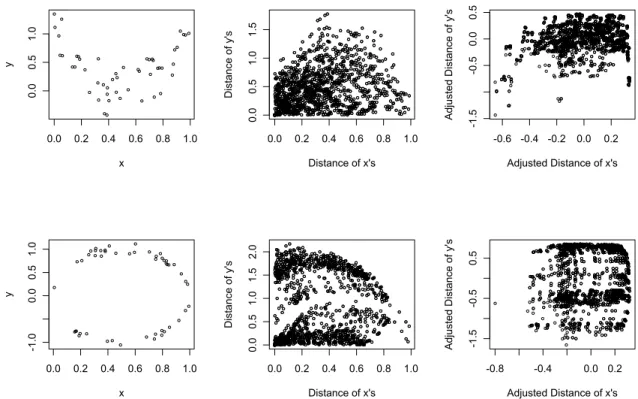
approach is intuitively sensible when the relationship is monotone, as sample pairs that are close on thex-axis should also be close on the y-axis. However, for non-monotone relationships, pairs of points that are close on the x-axis can be quite distant on the y-axis (Figure 1.1).
dCor satisfies several ideal theoretical properties (Sz´ekely et al. 2007). It is zero if and only if the two variables are independent and is the only method with an explicit formula to enjoy such property. Also, dCor can be used in higher dimensions and has an interpretation related to Brownian distances (Sz´ekely and Rizzo 2009).
0.0 0.2 0.4 0.6 0.8 1.0 0.0 0.5 1.0 x y
0.0 0.2 0.4 0.6 0.8 1.0
0.0
0.5
1.0
1.5
Distance of x's
Distance of y's
-0.6 -0.4 -0.2 0.0 0.2
-1.5
-0.5
0.0
0.5
Adjusted Distance of x's
Adjusted Distance of y's
0.0 0.2 0.4 0.6 0.8 1.0
-1.0 0.0 0.5 1.0 x y
0.0 0.2 0.4 0.6 0.8 1.0
0.0
0.5
1.0
1.5
2.0
Distance of x's
Distance of y's
-0.8 -0.4 0.0 0.2
-1.5
-0.5
0.5
Adjusted Distance of x's
Adjusted Distance of y's
Figure 1.1: Illustration of paired adjusted distances underlying dCor. (top row) Illus-tration of dCor for a quadratic relationship between x and y.(bottom row) A circular relationship between x and y. The adjusted paired distances show little correlation.
sample size it is able to detect a wide range of associations without being limited to any specific form. (ii) It is equitable in the sense that the value of the coefficient is similar for various forms of association that are equally ‘noisy’ in their departure from a functional relationship.
Simon and Tibshirani (2014) argued that such equitability may not be a desirable property while testing for general association, as it might lead to lower power of the test. However, recently there have been debates over the appropriate definition ofequitability and whether MIC truly enjoys that property (Kinney and Atwal 2014a;b).
the product of marginal distributions in the Cartesian product of balls around (x0, y0). The test uses as the test statistic a sum of n Pearson chi-square statistics where n is the number of paired observations. It can also be extended to higher dimensions. The method has been shown to be consistent asn grows larger and simulation studies were presented to demonstrate that it has high power against several alternatives.
1.1.5 Summary
To summarize, several tests of association have been found to perform well in terms of power in different situations. MIC, dCor and HHG are probably the most appealing in terms of their power against different alternatives, desirable theoretical properties and computational efficiency. However, their performance for small samples against various forms of associations has been relatively unexplored. In Chapter 2 we will present a comparison of these methods with our newly proposed method RankCover.
Our method RankCover is robust and powerful against different forms of associa-tion. The method has been applied on both simulated and real datasets and has been observed to perform better than competing methods in many situations. It is truly ‘general’ in the sense that it does not depend on the distributions of the two variables under consideration, and has the potential to detect any departure from independence.
1.2 Control of False Discovery Rate for Grouped Hypotheses
behavior under dependency, and to accommodate certain dependency structures. Often such hypotheses form into groups that exhibit different properties. The control of FDR without considering the group classification has the potential problem of over or under sensitivity as significant instances of one group might be hidden among the nulls of another group, and insignificant instances might look like significant (Cai and Sun 2009, Efron 2008).
FDR based approaches have also been studied in the domain of interval estimation (Benjamini and Yekutieli 2005, Jung et al. 2011, Zhao and Gene Hwang 2012). How-ever, we will focus on the methods controlling FDR in the grouped hypothesis setting, especially considering the applications for expression quantitative trait loci (eQTL) data.
1.2.1 Classical methods and family-wise error rate
Methods to control type I error, after considering the effects of multiple testing, are more than fifty years old and include the Bonferroni method (Dunn 1961) and Sidak method of multiple comparison (ˇSid´ak 1967), being proposed after the works of Tukey and Scheffe in the 1950’s. The Sidak method assumes the hypotheses to be independent and can be highly conservative if the correlations are positive. The Bonferroni method does not assume independence and can be even more conservative. Holm (1979) introduced the concept of a stepped procedure that can be used to improve the Bonferroni or Sidak method to obtain less conservative control. Using a similar approach, Hochberg (1988) proposed a step up procedure to obtain higher power. The concept of ‘Family-Wise Error Rate (FWER)’ was formalized by Westfall and Young (1993). They also introduced a permutation based procedure, applicable to many datasets, which can control the FWER exactly at the target level under a permutation null.
m hypotheses and m0 of them are true null. Based on a particular rejection criterion, let R of them be rejected. The cross-classification of the truth and the decision is as shown in Table 1.1. Then, FWER is defined as the probability of making at least one false discovery, i.e. P(V ≥1).
True Null True Alternative Total
Rejected V S R
Accepted U T m−R
Total m0 m−m0 m
Table 1.1: Showing the cross-classification of true and false null hypothesis against the decision to accept or reject
1.2.2 The false discovery rate approach
following way.
F DR≤ m0
mq when hypotheses are independent,
F DR ≤ m0
mq when hypotheses are positively dependent
(PRDS), F DR≤ m0
mq(1 +
1 2 +
1
3 +...+ 1
m) for general dependence.
It is clear that the FDR control using the Benjamini-Hochberg LSU procedure can thus be extremely conservative if the proportion of true null hypotheses (m0/m) is not close to 1. Even though controlling FDR at the exact level may not always lead to the most powerful procedure (Cao et al. 2013), in most cases the power is reduced when a procedure controls the FDR at a lower level than the target. This observation inspired the idea of ‘adaptive’ procedures, where m0 is first estimated from the data and then the LSU procedure is used for a target level qm/mˆ0 (Benjamini and Hochberg 2000, Storey 2002, Black 2004). Such plug-in type procedures, even though valid as ‘oracle’ procedures, might not always control the FDR when m0 is estimated from the same data. Especially under dependency, the variability of the estimate of 1/m0 can be very high (Farcomeni 2007b, Blanchard and Roquain 2009). Benjamini et al. (2006), Blanchard and Roquain (2009), Benjamini et al. (2009), Gavrilov et al. (2009) proposed several adaptive methods which can be proved to control the FDR at the target level.
1.2.3 Extension and different approaches to FDR
and Yakovlev 2006, Schwartzman and Lin 2011). Owen (2005) has noted that the variance of the number of false discoveries might be greatly inflated under dependence. Yekutieli and Benjamini (1999) proposed a permutation based approach to take care of the dependence, but it is computationally burdensome for large number of hypothe-ses. Other procedures to take care of the dependence have been proposed including a hidden Markov model based approach by Sun and Cai (2009). They propose an ‘oracle’ procedure as well as an asymptotically optimal data-driven procedure, but the entire procedure requires a natural ordering of the hypotheses such that dependencies of null/alternative hypotheses may be exploited. Genovese and Wasserman (2004; 2002) extended the FDR approach and also introduced the idea of ‘False Negative Rate’ (FNR) which is the expected proportion of false negatives among all non-rejections (Genovese and Wasserman 2002). They proposed an optimal method which minimizes the FNR subject to a bound on FDR. Sun and Cai (2007) also provided an ‘oracle’ method based on a decision theoretic framework that minimizes FNR while controlling the FDR. They showed that when the method is data driven, it asymptotically attains the performance of the ‘oracle’ procedure.
situations. However, the FDR is widely seen as the most useful one, having the desirable properties under the most general conditions (eg Fdr or pFDR cannot be controlled when all the null hypotheses are true).
1.2.4 The empirical Bayes approach and local false discovery rate
The empirical Bayes approach uses a Bayesian set up assuming the null hypothe-ses to be Bernoulli random variables, but estimates the prior probabilityπ0 instead of assuming prior belief. Empirical Bayes methods use the advantages of both classical and Bayesian approaches and can be superior to both in many cases (Casella 1985). Efron et al. (2001b) introduced the empirical Bayes approach for controlling FDR in microarray datasets and mentioned that such approach has an easy appeal and inter-pretation. The model, known as two-groups model, can be used in other applications as well. With such a model, for a given dataz related to a hypothesis, the density can be written as a mixture density:
f(z) =π0f0(z) + (1−π0)f1(z) (1.1)
wheref0 and f1 are the densities under null and alternative, respectively. The adaptiv-ity is in inherent to such procedures since the estimatiionπ0 is equivalent to estimating m0 in the classical FDR setting.
The difficulty of using the empirical Bayes approach is to estimate the lfdr’s. The requirement of the estimation of the null density f0 has been discussed by many re-searchers (Efron 2004, Jin and Cai 2007, Schwartzman 2008) although in some cases it might be assumed to be a known distribution (Efron et al. 2001a).
1.2.5 Grouped Hypotheses
Grouped hypothesis testing is a special case of multiple testing where the hypotheses have a natural stratification and adjustments for multiple comparison is required not only within each group, but also for the existence of multiple groups. For instance, gene expression data can be grouped according to the ontologies (Ashburner et al. 2000). For cis-eQTL analysis, there is a natural grouping in terms of the different genes. Within each gene, there are several SNPs local to the gene with which the associations are tested. For eQTL studies such as GTEx (Lonsdale et al. 2013), it is often useful to find out whether there is any eQTL within a particular gene since genes are believed to be directly associated with the diseases. An example for expression data is presented by Heller et al. (2009) where gene-sets are thought of as units of interest and a method to find out gene-sets that are differentially expressed has been developed. Benjamini and Heller (2007) reports an example where the clusters are of more interest than individual locations in a neuro-imaging study. They propose an adaptive procedure to control the FDR for clusters, i.e. to control the proportion of clusters erroneously rejected out of all rejected clusters.
at same target level α. However, such choice of αi = α for each group is not optimal
(Cai and Sun 2009). Yang and Jeong (2013) has applied such a separate analysis approach to RNAseq data. The conditional lfdr based ‘oracle’ procedure (when the distributional information of each group is known) introduced by Cai and Sun (2009), when applicable, has been shown to be optimal in the sense that it controls the overall FDR and minimizes the overall FNR. When the parameters are unknown, they propose a data-driven procedure that is asymptotically equivalent to the ‘oracle’ procedure.
Most of the other methods use weighted p-value based approaches to combine p-values from different groups (Benjamini and Hochberg 1997, Genovese et al. 2006, Hu et al. 2010). Roeder and Wasserman (2009) showed that such weighted p-value based methods are robust to weight misspecification. Hu et al. (2010) proposed a ‘Group Benjamini Hochberg’ method, but it is limited by the assumption that the non-null distribution of different groups are same. Zhao and Zhang (2014) proposed another weightedp-value method where the weights are obtained by maximizing a power-related objective function. Wang et al. (2010) introduced a Hidden Markov Model based method for group testing and succesfully applied it to GWAS data. Another method targeted at GWAS data was proposed by Sun et al. (2006).
1.2.6 Application in eQTL studies
There have been a lot of studies regarding eQTL data over the past decade. eQTL mapping methods have rapidly moved from classical genetic methods for linkage or association mapping to modern computationally efficient algorithms. Wright et al. (2012) provides a review of the different eQTL mapping methods. While some of the researchers emphasize on the statistical modeling aspect (Kendziorski et al. 2006, Chen and Kendziorski 2007, Gelfond et al. 2007), other methods focus on developing fast and efficient algortithms for the huge eQTL datasets (Gatti et al. 2009, Shabalin 2012, Purcell et al. 2007).
The FDR controlling procedure due to Benjamini and Hochberg (1995) and the q-value approach by Storey and Tibshirani (2003) are the most common approaches
to control FDR in eQTL studies. Among other approaches, some clustering methods are used by Jia and Xu (2007) and Chun and Kele¸s (2009). However, the natural grouping defined by the genes in the eQTL data is relatively unexplored. Due to the large number of groups and large number of hypotheses within the groups, many group-testing methods become computationally burdensome for eQTL datasets. However, the methods might be simplified by making further assumptions considering the special structure of the eQTL data.
1.2.7 Summary
separately, the application of grouped hypothesis testing for eQTL data has not been well explored. The natural grouping of the eQTL data using the genes as groups has been largely ignored when applying multiple comparison techniques, except using com-putationally intensive method such as permutation (Ardlie et al. 2015). There might be assumptions that do not hold in general for grouped hypotheses, but hold in eQTL data due to its special structure. In Chapter 3, we will discuss how such special structure of the data can be used to develop new group testing methodologies for eQTL datasets.
Our methodRandom Effects model and testing procedure for Group-level FDR con-trol (REG-FDR) models the alternative for the eQTL data and controls the FDR by adaptive thresholding. Z-REG-FDR, an approximate version of REG-FDR, is also proposed which exhibits similar results with much improved computational speed. As Z-REG-FDR is very similar to REG-FDR, which is based on maximum likelihood es-timation, Z-REG-FDR is conjectured to have near-optimality properties in estimation due to its use of an approximate MLE. This method is not only very fast compared to other grouped hypothesis testing methods, but it also does not require the full data to fit the model. In fact, using only the p-values for each gene-SNP pair is sufficient to conduct the gene-level hypothesis testing and control of the FDR.
1.3 Overview of the thesis
CHAPTER 2: A PROCEDURE TO DETECT GENERAL ASSOCIATION
2.1 Motivation
Adapting ideas from spatial analysis, we proposeRankCover, a method that quanti-fies the concentration of (x, y) values by measuring the area covered by laying disks of a fixed radius over each point in the scatter plot of the ranks of the two variables. In the presence of association, this area is expected to smaller than that under independence. Therefore, a left tailed test is appropriate in this case.
RankCoverstarts by computing ranks of the originalxandyvalues, and we assume there are no tied values. The use of ranks considerably simplifies the problem, by placing the intervals between successive ranked values on a common scale. In addition, for ranked values, the null distribution depends only on the sample size n. Thus the only computation lies in computing the observed statistic, while the null distribution can be pre-computed and is applicable to any dataset of sizen.
Diggle’s F(δ) function as introduced in Diggle (1983) is the distribution function of the distance between a randomly chosen point in a region to the nearest observed point (xk, yk). To obtain an empirical estimate of theF(δ), the investigator conceptually lays
disks of radiusδon each point (xk, yk) and calculates the proportion of the surrounding
region covered by the union of the disks (Figure 2.1). Ifx and y are highly associated, the areas covered by the disks should be small, and therefore RankCover rejects only in the left tail of the statistic described below.
depend on the choice of the distance metric. For instance, Euclidean distance leads to circular equidistance contours, resulting in circular disks, while the disks are diamond-shaped for Manhattan distance (Figure 2.1).
0.0 0.2 0.4 0.6 0.8 1.0
0.0
0.2
0.4
0.6
0.8
1.0
A
x
y
0 10 20 30 40 50
0
10
20
30
40
50
B
Rank(x)
Rank(y)
0 10 20 30 40 50
0
10
20
30
40
50
C
Rank(x)
Rank(y)
0 10 20 30 40 50
0
10
20
30
40
50
D
Rank(x)
Rank(y)
Figure 2.1: Illustration ofRankCoverfor sample sizen= 50: A.Scatter plot of the two variables. B. Scatter plot on the rank scale C. Disks laid on the scatter plot on rank scale using Euclidean distance D. Disks laid on the scatter plot on rank scale using Manhattan distance.
2.2 The test statistic
The empirical estimate ofF(δ) can be obtained using the proportion of area covered by the discs. For a given sample ((x1, y1), ...,(xn, yn)), xk ∈ X, yk ∈ Y, k = 1,2, ..., n,
ˆ
F(δ) = A(δ)
|X × Y| (2.1)
Let (rk, sk) denote the ranks of thekth sample pair,k= 1,2, ..., n. The
correspond-ing version of ˆF for ranks is given by
ˆ FR(δ) =
AR(δ)
n2 (2.2)
whereAR(δ) is the area covered by union of disks placed at each of (rk, sk).
However, it is difficult to calculate the exact area covered by the union of disks due to the complex nature of possible intersections. Acknowledging the discrete nature of the ranks, we consider only then×ngrid of possible rank pairs, {1,2, ..., n} × {1,2, ..., n}, and whether each of these values on the grid is covered by at least one disk.
Rank(x)
Rank(y)
Figure 2.2: Showing the Grid based approach of RankCover
Definition 1. Define d(i, j, xk, yk) = distance between the point (i, j) on the grid and
Using this definition, a reasonable statistic for fixed δ is
ˆ
FRG(δ) =
1 n2
n X
i=1
n X
j=1
I(dij ≤δ), (2.3)
where I(.) is the indicator function. The grid-based empirical distribution function (EDF) for ranks ˆFRG(δ) can be considered as an approximation to ˆFR(δ).
The choice of disk size δ is an important consideration which has not been fully addressed in the spatial statistics literature. Diggle (1983) suggested computing the entire empirical distribution function (EDF) ˆF(δ) to develop a new summary statis-tic to compare against the null curve. However, this approach makes the procedure prohibitively computationally expensive, and we propose using a fixed δ=√n for Eu-clidean distance (Section 2.3), with slight modification under Manhattan distance. It is observed that there is very little difference in power to detect association between the method using the entire EDF and the statistic using a fixed δ =√n (Figure 2.3). In addition, we modify the statistic to account for edge effects of the grid, using an (n+dδe)×(n+dδe) grid extending beyond the range of the scatterplot. Here dδe is the smallest integer greater than or equal toδ. Finally, our modified test statistic is
T(δ) = 1 n2
n+dδe
X
i=1−dδe n+dδe
X
j=1−dδe
I(dij ≤δ), (2.4)
where the range of {i, j} reflects the outer boundaries of a larger region to account for edge effects. Note that the same divisorn2 is used allowingT(δ) to be greater than 1. T(δ) can be interpreted as the proportion or area covered by the disks as compared to the area of Rn, the n×n region which is the range of the original scatter plot.
area-based statistic.
Lemma 1. LetTA(δ)be the area based test statistic corresponding to T(δ)with areas of
the disks extending beyond the n×n square being taken into account. For δ=O(√n),
|TA(δ)−T(δ)|
a.s.
−−→0 as n → ∞.
Proof. For a single disk with radius δ, by the Gauss circle problem (Gauss 1986), the difference of its actual area and its lattice based approximation N(δ) is bounded by 2√2πδ.
Therefore, for δ = O(√n), with probability 1, |TA(δ)−T(δ)| ≤ 2n √
2πδ
n2 = O(
1
√
n)→ 0
asn → ∞. .
The implication of this lemma becomes obvious in (Section 2.6) when we discuss large sample properties of RankCover. In small samples, the two statistics TA(δ) and
T(δ) might be quite different. However, there is no reason to believe that one is inferior to the other in small samples sinceT(δ) actually computes similar disk coverage statistic for a different disk shape that looks like a polygon.
0.2 0.4 0.6 0.8 1.0
0.0
0.4
0.8
Linear
Noise Level
Power
0.2 0.4 0.6 0.8 1.0
0.0
0.4
0.8
Quadratic
Noise Level
Power
0.2 0.4 0.6 0.8 1.0
0.0
0.4
0.8
Circle
Noise Level
Power
RankCover AUC method
Figure 2.3: Showing the comparison of power of the method using the area under the EDF (AUC method) and that of the method using δopt =
√
2.3 Choice of parameters and distance metric
The choice of the disc size δ is an important consideration. We have proposed the use of a single optimum choice of δ as opposed to the whole δ versus ˆF(δ) curve used by Diggle (1983). The argument for choosing δopt =
√
n for Euclidean distance and δ=pπ
2nis somewhat heuristic, but based on empirical observations for several sample sizes.
100 200 300 400 500
5
10
15
20
A
n
E
(
D1
)
E(D1) n
100 200 300 400 500
10
15
20
25
30
35
40
45
B
n
E
(
D2
)
E(D2) 2 n
Figure 2.4: Showing the expected δ for which A. T(D1) = 1 B. FˆRG(D1) = 1
The external region beyond Rn is used to take care of the edge effects. However,
it is the behavior of the disks insideRn that primarily differentiates between null and
alternative. While trying to find a disk size that will enhance this difference the most, it is reasonable to believe that increasing disk size will not provide much of information onceRnis completely covered. Since the computational cost increases with the increase
of the disk size, one would like to stop increasing the disk size when it stops providing much information. Therefore, we try to find out the disk size for whichRnis completely
covered.
Further-more, Hall et al. (1985) proved that for a Boolean process (Discussed in Section 2.6), the probability of coverage is 1 if the area of the disk an satisfies
an/n−log(n)−log(log(n))→ ∞ as n→ ∞. (2.5)
It is evident that for δ = nα, this condition is satisfied if and only if α > 1
2. Even though this result does not have a direct implication in our case, it is suggestive of the order of the ‘stopping’ disk size. To further explore the stopping condition, we used simulated data and calculated the expectation of two variables D1 and D2 defined as below.
D1 = Smallest disk size for which the realizedT(D1)>1. D2 = Smallest disk size for which the realized ˆFRG(D1)>1.
Figure 2.4 Shows that bothE(D1) and E(D2) are probably of the order
√
n.
0 5 10 15 20
0.0
1.0
2.0
δ
Mean
δopt
0 5 10 15 20
0.00
0.02
0.04
δ
Standard Deviation
δopt
0 5 10 15 20
0.00
0.01
0.02
0.03
δ Coefficient of Variation δopt
Figure 2.5: Showing the mean, sd and coefficient of variation of T(δ) for sample size 50 (Euclidean distance is used)
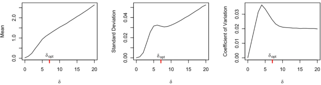
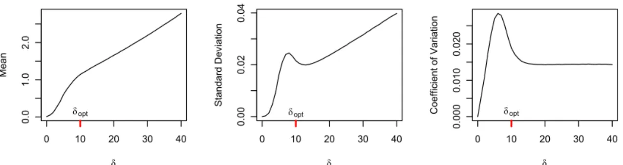
minimum of the standard deviation represents a good choice for δ. We also note that the point where the expectation curve changes the curvature is approximately the same point as the local minimum of the standard deviation, and the coefficient of variation is almost constant beyond this point. However, there is no closed form expression for this point of local minimum. From simulations under different sample sizes, we have established that such local minima occur near δ = √n for Euclidean distance, and propose it as our choice ofδopt.
0 10 20 30 40
0.0
1.0
2.0
δ
Mean
δopt
0 10 20 30 40
0.00
0.02
0.04
δ
Standard Deviation
δopt
0 10 20 30 40
0.000
0.010
0.020
δ
Coefficient of Variation δopt
Figure 2.6: Showing the mean, sd and coefficient of variation of T(δ) for sample size 100 (Euclidean distance is used)
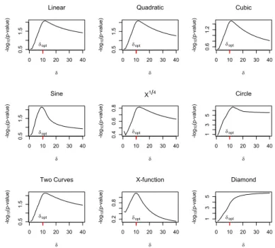
Thus, there is enough reasons to believe that the optimalδshould be of the order√n even though the minimum of the standard deviation is not exactly at√n. Rather, the minimum can be better empirically modeled as√n+pn/5−10 for sample sizes up to 500 (Figure 2.7). However, all these heuristic arguments deal with the behavior of the test statistic under null. We have also compared its power against different alternatives for varyingδ. Figure 2.8 shows the average p-value in−log10scale for different forms of association. Clearly there is no singleδfor which the power is maximized. However, the power for δ =√n is close to the maximum power achieved in all the cases. Therefore we conclude that it is not possible to find out a disk size that is ‘optimum’ in the true sense, but δopt =
√
100 200 300 400 500 5 10 15 20 25 30 35 n Argmin δ sd ( T ( δ ))
δ for which the standard deviation is minimum
δopt= n+ n 5−10
Figure 2.7: Showing theδfor which standard deviation ofT(δ) is minimum for different sample sizes
0 10 20 30 40
0.5 1.5 Linear δ -log 10 (p-value) δopt
0 10 20 30 40
0.5 1.5 Quadratic δ -log 10 (p-value) δopt
0 10 20 30 40
0.6 1.2 Cubic δ -log 10 (p-value) δopt
0 10 20 30 40
0.5 1.5 Sine δ -log 10 (p-value) δopt
0 10 20 30 40
0.4
0.6
0.8
X1 4
δ
-log
10
(p-value)
δopt
0 10 20 30 40
1 3 5 Circle δ -log 10 (p-value) δopt
0 10 20 30 40
0.5 1.5 Two Curves δ -log 10 (p-value) δopt
0 10 20 30 40
0.2 0.8 X-function δ -log 10 (p-value) δopt
0 10 20 30 40
1 3 5 Diamond δ -log 10 (p-value) δopt
Figure 2.8: Showing the Average p-value using different disk sizes when testing against various forms of association
only through the area of the disk (also shown by Hall (1988) for Boolean process), and so we use δopt =
pπ
For the distance metric d, we consider here both Euclidean and Manhattan dis-tances, for which simulations show similar performance (Section 2.7.1). However, the Manhattan distance has advantages in approximating tail areas since the rejection thresholds follow a sawtooth pattern (Figure 2.9), with jump points occurring at the values of n where [δ] changes. For large values of n, to reduce computation, one can perform direct simulation for the values of n at, and just prior to, the jump points, followed by linear interpolation for remaining values ofn. Therefore we recommend its use and here present results using Manhattan distance.
100 200 300 400 500
1.05
1.10
1.15
1.20
Sample Size
5% Quantile
Obtained by actual simulation Obtained by linear interpolation
Figure 2.9: Showing the pre-computed thresholds for the RankCover method with Manhattan distance. 100000 simulations were used to calculate the thresholds in each case. Simulations were performed for n = 20, ...,100. For large values of n, to reduce computation, tables were generated by (i) performing direct simulation for the values of n at, and just prior to, the jump points, followed by (ii) linear interpolation for remaining values of n.
2.4 Fast Computation of the test statistic
disk. Then the prototype matrix is used to “punch” a hole at each of the sample points (Figure 2.10).
Scatter plot of ranks Prototype matrix Coverage
Figure 2.10: Showing the fast computation ofRankCover
2.5 Exact expectation of the RankCover statistic for Manhattan distance
We exploit the desirable properties of Manhattan distance to obtain the exact value ofE(Tn(δ)). Let us define the random variablesIij,i= 1,2, ..., n;j = 1,2, .., n,for each
point (i, j) on the grid. Iij is 1 if there is any sample point within the distance δ from
(i, j) and 0 otherwise.
Figure 2.11: Schematic to illustrate calculation of P(Iij = 1) for 1≤i≤n,1≤j ≤n.
Let us consider the case where the δ-ball lies completely within the Rn. From
P(Iij = 1) = 1− n−n1, 0< δ <1
P(Iij = 1) = 1− n−n3nn−−21nn−−32, 1≤δ <2
P(Iij = 1) = 1− n−n5nn−−41nn−−52nn−−43nn−−54, 2≤δ <3 and so on.
In general, if [δ] =k,
P(Iij = 1) = 1−
(n−2k−1)k+1(n−2k)k
(n)(2k+1)
(2.6)
It becomes more complicated when a part of theδ-ball lies outside then×n region. It is difficult to obtain a simplified formula like above, but similar counting procedure can be used to get the expression of the expectation.
Let [δ] =kand nare given. We need to find pij(k, n) = P(Iij = 1) for a given point
(i, j) on the grid. Define
nl(t, k, n) = min{t−1, k}
nr(t, k, n) = min{n−t, k}
and
n(i, k, n) = 1 +nl(t, k, n) +nr(t, k, n)
.
nl(t, k, n) is the number of points at the left of (t, .) on the same horizontal line
within the δ-ball as well as within the n×n region. nr(t, k, n) is the number of such
points at the right and n(t, k, n) is the number of such points on that horizontal line. Let I(t, k, n) denote the index vector of the relative positions of the n(t, k, n) points with respect to (t, .). We assume that I(t, k, n) consist of the sorted absolute values and call the rth element of it Ir(t, k, n). For example, in Figure 2.11, for δ = 2,
I(6,2,12) = (0,1,1,2,2).
pij(k, n) = 1− n(i,k,n)
Y
r=1
n−r+ 1−n(j, k−Ir(i, k, n), n)
n−r+ 1 (2.7)
Figure 2.12: Showing the existence of (i0, j0) for a point (i, j) outside the n×n region Equation 2.7 applies to any point (i, j) within the n×n region. For (i, j) outside the region, there exists a point (i0, j0) (See Figure 2.12) on the edge of the region such that
pij(k, n) =pi0j0(k0, n)
.
Here
i0 =I{i <1}+nI{i > n}+iI{1≤i≤n},
j0 =I{j <1}+nI{j > n}+jI{1≤j ≤n},
k0 =k− |i−i0| − |j−j0|.
2.6 Large sample properties of RankCover
The computation of theRankCoverstatistic might be quite slow if the sample size is very large. For instance, with n >10000, the Monte Carlo simulations to produce the null distribution of the test statistic becomes computationally expensive. The testing procedure will be much simpler and faster if the large sample theoretical distribution of RankCover can be determined. In the following sections we discuss the established large sample results pertaining to the theory of coverage process and RankCover’s relationship with them. Euclidean distance is considered as the distance metric, but the same arguments can be easily shown to apply for Manhattan distance too.
2.6.1 Coverage Process
The theory of coverage process is related to the idea of RankCover. In a simple set up, a coverage process can be thought of as a countable sequence of sets in an Euclidean space (Section 2.6). Suppose P = {ξ1, ξ2, ..} is a countable collection of points in Rk (which might be a stochastic point process (Karr 1991)), and {S
1, S2, ...}
is a countable collection of non-empty sets (might be random sets). If ξi +Si denotes
the set {ξi+x : x ∈ Si}, then C = {ξi +Si : i = 1,2, ...} is a coverage process. The
union of all sets in C is known as a ‘germ-grain’ model where the points ξi are referred
to as ‘germs’ and the sets Si as ‘grains’. If P is a stationary Poisson process and Si’s
are iid random sets independent of P, thenC is known as a ‘Boolean’ process.
In a simpler version of coverage process, which is relevant to our problem, the sets Siare all equal to a fixed setS(in our case, the disks), and the point process{ξ1, ξ2, ...} is assumed to be generated from a regionR, which is known as the ‘experiment space’. WhileC =∪i(ξi+Si) is called the total coverage, the vacancy within a subset Rof Rk
is defined as
Note that the setR does not have to be same as the experimental spaceRalthough most of the coverage process literature deals with the vacancy V(R) within R. The proportion of vacancy within R is called the porosity, and is directly related to the wayRankCover is formulated. The major difference is the point process inRankCover which is not a Poisson process due to the use of ranks.
Various researchers has found out moments and limiting distributions of vacancy under different conditions. Hall (1985) proved the aymptotic normality of vacancy for a Boolean process and provided the expressions for its mean and variance. Moran (1974) computed limiting distributions of coverage assuming that the points are generated from a normal distribution. Similar work has been done by Miles (1969), Ailam (1966), Hall (1984). However, most of the work in this area has assumed that the points are generated independently. In the presence of dependency, the derivation of these limit theorems becomes extremely complicated (Hall 1988). Little work has been done with dependent cases, and very specific situations are handled in the few attempts that have been made (Moran 1973). Those situations are not similar toRankCover.
We present a few early results with the conjecture that as n becomes large, the dif-ference betweenRankCover and the case considered by Hall (1985) becomes negligible. We provide empirical evidence to support the conjecture that for very largen the two distributions to become similar.
2.6.2 Asymptotic Negligibility of the edge effect
we consider the coverage beyond the experimental space R. Therefore the result due to Hall (1984) does not directly apply. The following lemma proves that the edge effect for RankCoverconverges to zero as n becomes large.
Lemma 2. For δ =O(√n), |T(δ)−FˆRG(δ)| a.s.
−−→0 as n → ∞.
Proof. We consider Euclidean distance as the distance metric. Let δ =O(√n) be the radius of the disks, and k = [δ]. For any circular disk lying partially outsideRn, there
exists a rectangle within which the circular portion can be inscribed. Considering the area of such rectangle as an upper bound for the area of the portion of the circle, we obtain, with probability 1,
|T(δ)−FˆRG(δ)| ≤4{2δ2 + 2δ(δ−1) + 2δ(δ−2) +...+ 2δ(δ−k)}
= 8δ{(k+ 1)δ− k(k2−1)}=O(√1
n)→0 as n→ ∞.
One should note that such convergence is clearly quite slow and the sample size needs to be very large in order for the edge effect to be negligible for practical purposes.
2.6.3 Asymptotics of coverage for Boolean process
Hall (1985) proved the aymptotic normality of vacancy V for Boolean process and provided the expressions for its mean and variance. The expression for the mean and variance of the proportion of coverageC follows directly from those. For δ =√n, the expressions are
E(C) = 1−exp(π) (2.8)
σ2 =nV(C) = πe−2π(8
ˆ 1
0
u{e2πJk(u)−1}du−π) = πe−2π(8×0.997216−π), (2.9)
whereJk(u) = π1(π2 −sin−1(u)− 12sin(2sin−1u)).
√
n(C−E(C))−→d N(0, σ2). (2.10)
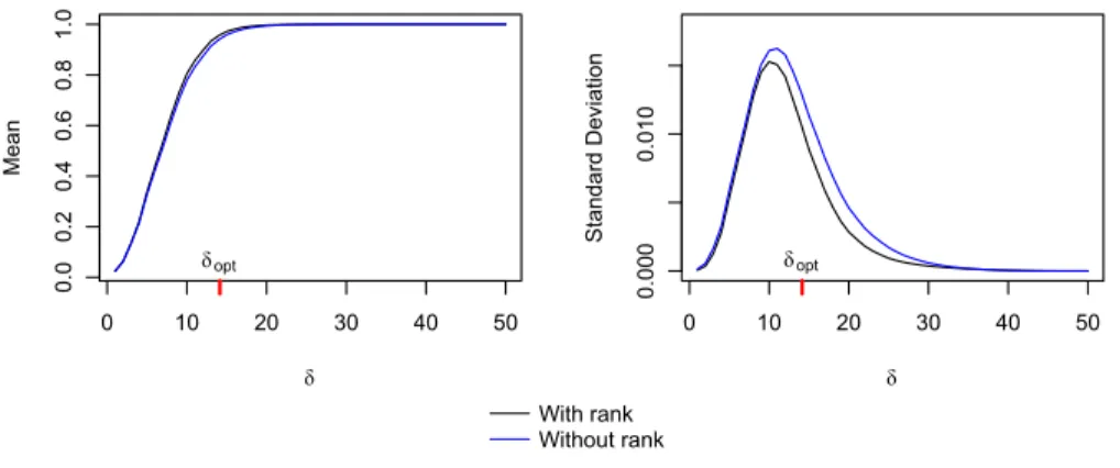
However, these results do not directly apply toRankCover, and the difference might be substantial even for moderately large n (Figure 2.13).
0 10 20 30 40 50
0.0
0.2
0.4
0.6
0.8
1.0
δ
Mean
δopt
0 10 20 30 40 50
0.000
0.010
δ
Standard Deviation
δopt
With rank Without rank
Figure 2.13: Showing the difference in mean and standard deviation between total coverageC for Boolean process and the RankCover statistic.
2.6.4 Applicability of the results to RankCover
If it can be shown that the difference between the total coverage as in Hall (1985) and theRankCoverstatistic becomes negligible asn becomes large, then Equation 2.8, Equation 2.9 and Equation 2.10 can be conveniently used for largen to test for general association.
Let us examine the difference between the joint distributions of ((x1, y1), ...,(xn, yn))
under the null in both cases. If ((x1, y1), ...,(xn, yn)) are independent samples from a
bivariate discrete uniform distribution over{1,2, ..., n} × {1,2, ..., n}, the joint density is
f1((x1, y1), ...,(xn, yn)) =
1
If ((x1, y1), ...,(xn, yn)) are the ranks, the joint density becomes
f2((x1, y1), ...,(xn, yn)) =
1
n!2. (2.12)
The Hellinger distance between the two distributions is H(f1, f2) =
r
1−
q n!2 n2n →
1 as n → ∞. Therefore, the effect of rank does not wash away as n becomes large. However, the effect of rank on the test statistic might still be asymptotically negligible. But, it is difficult to prove or disprove it analytically.
0 2000 4000 6000 8000 10000
-0.020
-0.010
0.000
A
n
Mean
0 2000 4000 6000 8000 10000
0.12
0.14
0.16
0.18
0.20
B
n
Standard Deviation
With Rank Without Rank
Large sample approximation
Figure 2.14: Showing the A. mean and B. standard deviation of √n(C−E(C)) for Boolean process and the corresponding statistic for ˆFRG(δ).
To see the differences, we examined the behavior of coverage proportion C as in Hall (1985) and the RankCover test statistic for simulated datasets (Figure 2.14, Fig-ure 2.15). FigFig-ure 2.14 indicates that the expectation and variance of C and ˆFRG(δ)
might be sufficiently close for very large n, but there is no conclusive proof. By Lemma 2, this implies that C and T(δ) might also be close asymptotically. How-ever, it requires even larger sample size for them to be close enough (Figure 2.15). Based on Figure 2.14, we suggest that for sample sizes in the range 2000-10000, ˆFRG(δ)
n= 2000,5000 and 10000 were 0.045,0.054 and 0.053.
0 2000 4000 6000 8000 10000
0.00
0.10
0.20
0.30
A
n
Mean
0 2000 4000 6000 8000 10000
0.16
0.18
0.20
0.22
B
n
Standard Deviation
Edge effect corrected Large sample approximation
Figure 2.15: Showing the A. mean and B. standard deviation of √n(C−E(C)) for Boolean process and the corresponding statistic for T(δ).
2.7 Simulation Results
2.7.1 Comparison of different methods for simulated datasets
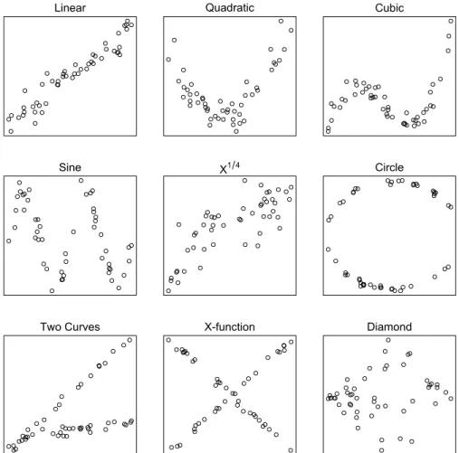
Following the simulation procedure used in Simon and Tibshirani (2014), we have simulated pairs of variables with several canonical dependency relationships (Figure 2.16) and with varying noise levels. In each scenario, theX values were simulated iid from a uniform distribution, while the noise distribution was Gaussian. However, the overall results were similar for other distributional forms.
The simulation results indicate thatRankCoverand dCor have some complementary characteristics, and so we additionally propose a hybrid statistic using results from RankCoverand dCor. The hybrid method uses the minimum p-value fromRankCover and rank-based dCor as a new statistic.
Linear Quadratic Cubic
Sine X1 4 Circle
Two Curves X-function Diamond
Figure 2.16: Showing the scatter plots for different relationships between the pair of variables (low noise level).
RankCover performs better than MIC in all the situations we have considered. It is found to be more powerful than dCor and HHG in several cases while these methods are found to be more powerful in other cases. Even when dCor or HHG is more powerful, RankCover still has reasonable power to identify the association. We have tested that these observations hold true for varying sample sizes, levels of noise, and functional forms for the originating X and noise distributions.
0.2 0.4 0.6 0.8 1.0 0.0 0.4 0.8 Linear Noise Level Power
0.2 0.4 0.6 0.8 1.0
0.0 0.4 0.8 Quadratic Noise Level Power
0.2 0.4 0.6 0.8 1.0
0.0 0.4 0.8 Cubic Noise Level Power
0.2 0.4 0.6 0.8 1.0
0.0 0.4 0.8 Sine Noise Level Power
0.2 0.4 0.6 0.8 1.0
0.0
0.4
0.8
X1 4
Noise Level
Power
0.2 0.4 0.6 0.8 1.0
0.0 0.4 0.8 Circle Noise Level Power
0.2 0.4 0.6 0.8 1.0
0.0 0.4 0.8 Two Curves Noise Level Power
0.2 0.4 0.6 0.8 1.0
0.0 0.4 0.8 X-function Noise Level Power
0.2 0.4 0.6 0.8 1.0
0.0 0.4 0.8 Diamond Noise Level Power
dcor RankCover Hybrid MIC HHG
Figure 2.17: Showing the power of different methods (type-Iα = 0.05) against different relationships at varying noise levels (Manhattan distance),n = 50.
is less sensitive to non-monotone relationships for the reasons described earlier (Sec-tion 1.1.4). We have also observed that with monotone rela(Sec-tionships, the Spearman’s rank correlation is as powerful as dCor. Therefore, one might simply use Spearman’s rank correlation if there is prior knowledge that the relationship is monotone. On the other hand,RankCoveris more sensitive to local clustering of points rather than trends. Thus, it is powerful against even non-monotone relationships like cubic, circular or the “X” relationship.
0.2 0.4 0.6 0.8 1.0 0.0 0.4 0.8 Linear Noise Level Power
0.2 0.4 0.6 0.8 1.0
0.0 0.4 0.8 Quadratic Noise Level Power
0.2 0.4 0.6 0.8 1.0
0.0 0.4 0.8 Cubic Noise Level Power
0.2 0.4 0.6 0.8 1.0
0.0 0.4 0.8 Sine Noise Level Power
0.2 0.4 0.6 0.8 1.0
0.0
0.4
0.8
X1 4
Noise Level
Power
0.2 0.4 0.6 0.8 1.0
0.0 0.4 0.8 Circle Noise Level Power
0.2 0.4 0.6 0.8 1.0
0.0 0.4 0.8 Two Curves Noise Level Power
0.2 0.4 0.6 0.8 1.0
0.0 0.4 0.8 X-function Noise Level Power
0.2 0.4 0.6 0.8 1.0
0.0 0.4 0.8 Diamond Noise Level Power
dcor RankCover Hybrid MIC HHG
Figure 2.18: Showing the power of different methods (type-Iα = 0.05) against different relationships at varying noise levels (Euclidean distance),n = 50.
and dCor, as the two methods appear powerful in different situations. Formally, a new statistic is definedshybrid = min(pdCor, pRankCover), wherepRankCover is the p-value
obtained by usingRankCover, and pdCor is that using dCor on (rank(x), rank(y)). The
p-value for the hybrid method is phybrid = P(Shybrid ≤ shybrid). As with RankCover,
the p-value can be obtained by using pre-computed simulations. The hybrid method, as expected, is always less powerful than the most powerful statistic for each scenario, but seems to be robust against all forms of association investigated.
RankCoverand the hybrid method to detect periodic relationships and non-functional relationships makes it very useful against such alternatives. The fact that RankCover is especially powerful against periodic relationships will be reinforced by the results in Section 2.8.3 and Section 2.8.4.
We summarize by emphasizing thatRankCoverand the hybrid method are powerful and robust in comparison to competing methods, and that these simulations cover a large range of relationships and noise levels. The broad conclusions are also not very sensitive to the marginal distributions of X and the error distributions.
0.2 0.4 0.6 0.8 1.0
0.0 0.4 0.8 Linear Noise Level Power
0.2 0.4 0.6 0.8 1.0
0.0 0.4 0.8 Quadratic Noise Level Power
0.2 0.4 0.6 0.8 1.0
0.0 0.4 0.8 Cubic Noise Level Power
0.2 0.4 0.6 0.8 1.0
0.0 0.4 0.8 Sine Noise Level Power
0.2 0.4 0.6 0.8 1.0
0.0
0.4
0.8
X1 4
Noise Level
Power
0.2 0.4 0.6 0.8 1.0
0.0 0.4 0.8 Circle Noise Level Power
0.2 0.4 0.6 0.8 1.0
0.0 0.4 0.8 Two Curves Noise Level Power
0.2 0.4 0.6 0.8 1.0
0.0 0.4 0.8 X-function Noise Level Power
0.2 0.4 0.6 0.8 1.0
0.0 0.4 0.8 Diamond Noise Level Power dcor Spearman
2.7.2 Comparison of dCor and Rank Correlation
Distance Correlation (dCor) seems to be the most powerful method among all the competing methods when the relationship is monotone (eg linear, X1/4, Two curves). However, further simulations show that even Spearman’s rank correlation is equally powerful in those cases (Figure 2.19). Therefore, if we have prior knowledge that the relationship is monotone, then we do not gain power by using the more recently developed methods anyway, and could use Spearman’s rank correlation instead. We note that Spearman’s rank correlation does not have much “generality” in the sense that it is not powerful against non-monotone alternatives. However, dCor has also been shown to have similar limitations.
2.8 Application on Real Data
In addition to simulated data, we illustrate all the approaches on several real datasets.
2.8.1 Example 1: Eckerle4 data
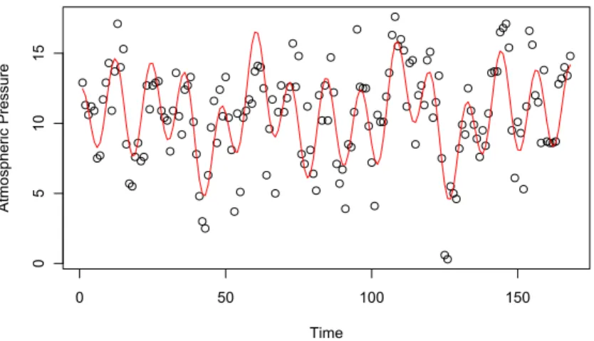
We show data from a study of circular interference transmittance (Eckerle 1979) from the NIST Statistical Reference Datasets for non-linear regression. The data were analyzed by Sz´ekely and Rizzo (2009) to illustrate dCor, and contain 35 observations on the predictor variable wavelength and the response variable transmittance.
Figure 2.20 shows the scatter plot of the predictor and the response along with the fitted curve (NIST StRD for non-linear regression) based on the model
y = β1 β2exp{
(x−β3)2
2β2
2 }+,
whereβ1, β2 >0, β3 ∈Rand is random Gaussian noise.