DOI: 10.1051/0004-6361:20040227 c
ESO 2005
Astrophysics
&
Dust cloud formation in stellar environments
II. Two-dimensional models for structure formation around AGB stars
P. Woitke
1,2and G. Niccolini
31 Sterrewacht Leiden, PO Box 9513, 2300 RA Leiden, The Netherlands e-mail:[email protected]
2 Zentrum für Astronomie und Astrophysik, TU Berlin, Hardenbergstrase 36, 10623 Berlin, Germany 3 Observatoire de la Côte d’Azur, Département Fresnel UMR 6528, BP 4229, 06034 Nice Cedex 4, France
Received 9 February 2004/Accepted 16 November 2004
Abstract.This paper reports on computational evidence for the formation of cloud-like dust structures around C-rich AGB stars. This spatio-temporal structure formation process is caused by a radiative/thermal instability of dust-forming gases as identified by Woitke et al. (2000, A&A, 358, 665). Our 2D (axisymmetric) models combine a time-dependent description of the dust formation process according to Gail & Sedlmayr (1988, A&A, 206, 153) with detailed, frequency-dependent continuum radiative transfer by means of a Monte Carlo method (Niccolini et al. 2003, A&A, 399, 703) in an otherwise static medium (u=0). These models show that the formation of dust behind already condensed regions, which shield the stellar radiation field, is strongly favoured. In the shadow of these clouds the temperature decreases by several hundred Kelvin, which triggers the subsequent formation of dust and ensures its thermal stability. Considering an initially dust-free gas with small density inhomo-geneities, we find that finger-like dust structures develop which are cooler than the surroundings and point towards the centre of the radiant emission, similar to the “cometary knots” observed in planetary nebulae and star formation regions. Compared to a spherical symmetric reference model, the clumpy dust distribution has little effect on the spectral energy distribution, but dominates the optical appearance in near IR monochromatic images.
Key words.instabilities – radiative transfer – ISM: dust, extinction – stars: AGB and post-AGB – stars: circumstellar matter – stars: mass-loss
1. Introduction
Dusty gases in space are often remarkably inhomogeneous. Numerous observations of various dust-forming objects like the circumstellar environments of AGB and post-AGB stars, R Coronae Borealis stars, planetary nebulae, the ejecta of no-vae and supernono-vae, and even the hot winds generated by Wolf-Rayet stars, have shown that a dust-forming medium usually possesses a clumpy internal structure. Reviews of such obser-vations are given by Lopez (1999) and Woitke (2001).
The best-studied object in that respect is probably the in-frared carbon star IRC+10216. Several infrared speckle obser-vations of its innermost dust formation and wind acceleration zone show direct evidence for an irregular, possibly cloudy dust distribution around this late-type AGB star (Weigelt et al. 1998; Haniff& Buscher 1998; Tuthill et al. 2004). Recently, Monnier et al. (2004) published further high-resolution images of dust shells around evolved stars which clearly show large-scale in-homogeneities. Additional evidence for wind asymmetries can be deduced from long-term JHKL lightcurves. Concerning the carbon star II Lup, Feast et al. (2003) argue for a restricted epoch of dust formation in a limited region along the line of sight, in order to explain a large-amplitude long-term decrease
in J whereas no corresponding increase in K and L was de-tected. Direct IR imaging and multi-wavelength IR lightcurves of the oxygen-rich red giant L2Pup point to similar wind asym-metries (Jura et al. 2000).
Further hints of inhomogeneities in the environments of AGB stars are given by the patchy SiO maser spots observed in oxygen-rich Mira variables (e.g. TX Cam, Diamond & Kemball 2003). On a larger scale, CO rotational emission lines provide evidence for local density enhancements in the winds of late-type stars, e.g. concerning the carbon star TX Psc (Heske et al. 1989) or in high-resolution observa-tions of the detached shell of TT Cyg (Olofsson et al. 2000). Observations with higher spatial resolution, using instruments like the V
, N
or A
, can be expected to reveal even more details in the near future.1D models), or whether they might break apart into clouds due to instabilities. We focus in this paper on the second possibil-ity and study the two-dimensional time-dependent behaviour of the dust/gas mixture just during the formation of a new dust shell.
Clumpiness may also play a vital role for the photo-chemistry during the AGB → PPN → PN transition phase. Opaque clumps can suppress the photodissociation of certain molecules like benzene, such that their existence has been pro-posed to be an indicator for inhomogeneities with large density contrasts (Redman et al. 2003).
Regarding other classes of objects, numerous opaque struc-tures have been discovered in proto-planetary nebulae (e.g. the Helix nebula NGC 7293 and the Eskimo nebula NGC 2392) as well as in star formation regions (e.g. the Orion nebula). These neutral, dense, probably dusty regions, designated as “cometary knots”, “globules” or “proplyds”, are located at the head of radially aligned linear structures in these nebulae and are particularly well visible in high resolution images of emis-sion line ratios like [OIII]/Hα(O’Dell 2000).
The physical cause of the observed clumpiness is still puz-zling. In Paper I of this series (Woitke et al. 2000), we for-mulated the hypothesis that a radiative/thermal instability in dust-forming gases can provoke self-organisation of the mat-ter, which is possibly involved in the formation of the observed structures. This instability is characterised by a physical con-trol loop between the radiative transfer, which determines the temperature structure of the medium, and the dust formation, which determines its opacity (see Fig. 1 in Paper I).
This paper reports on computational evidence for this hypothesis. In Sect. 2 we outline the concept of our static model for the environment of a C-rich AGB star, which com-bines a time-dependent treatment of dust formation with two-dimensional radiative transfer. Section 3 shows and discusses the results, including the calculated optical appearance of a clumpy dust distribution in the spectral energy distribution and in monochromatic images. In Sect. 4 our conclusions are drawn.
2. The model
The spatio-temporal evolution of the dust component in the circumstellar environment of a C-rich AGB star is simulated by means of a 2D (axisymmetric) time-dependent model. Our aim is to present a new physical effect, namely that the radia-tive/thermal instability explained in Paper I can excite large-scale self-organisation of the dust-forming medium. We do not intend to model any specific object. Instead, we are interested in what kind of spatial structures might develop, and we want to identify which physical control mechanisms are responsible for the structure formation process.
According to this purpose, the radiative, chemical and physical processes directly involved in the instability must be modelled as completely and accurately as necessary. In our two-dimensional approach, a precise radiative transfer calcula-tion requires large computacalcula-tional efforts (see Sects. 2.5 and 2.6 for details) and with our current approach, we are already at the computational limit of today’s super-computer facilities.
Therefore, the remaining parts of the model must be kept com-parably simple. For these reasons, we assume that the gas/dust mixture is static (u=0) and focus only on the time-dependent dust-chemistry and the radiative transfer. Another reason for this approach is that we want to study the pure effect of the instability, which might become entangled with other dynam-ical instabilities, if hydrodynamics were included. Regarding the stellar parameters of our sample model (see Fig. 2), in par-ticular the luminosity L =3000 L, it is not certain whether enough radiation pressure can be provided to drive a dust-driven outflow, i.e. the circumstellar environment of such stars may not be so far from hydrostatic.
Our approach makes it possible to explore the qualitative behaviour of the dust component in AGB star winds beyond spherical symmetry. This is, as far as we know, the first multi-dimensional and time-dependent (though static) model for dust formation around a cool star that includes the important feed-back of dust on the temperature structure of the medium via radiative transfer effects. Other authors have mainly focused on the dynamics and the wind acceleration by means of spheri-cally symmetric models (e.g. Winters et al. 2000; Höfner et al. 2003; Sandin & Höfner 2003). Freytag & Höfner (2003) have passively integrated the dust moment equations in first 3D sim-ulations, without feedbacks.
2.1. Gas density distribution
The time-dependent simulations of dust formation and radia-tive transfer are carried out for a restricted model volume, which covers the outer atmospheric layers of the star mainly responsible for the dust formation. Within this volume, the particle density of hydrogen nuclei nH[cm−3] (mass density
ρ=1.4 amu·nHfor solar element abundances) is initially set and left unchanged during the time-dependent calculations, ac-cording to our assumption of a static medium. We consider an exponentially decreasing density distribution in the radial di-rection with small spatial inhomogeneities. Our motivation for this type of radial density-dependence originates from 1D mod-els (e.g. Fleischer et al. 1995), which show an exponential rather than a 1/r2-dependence close to the star, just before the formation of a new dust shell begins1.
nH(r)=nH(r0)·exp
−r−r0
Hρ +δ(r)
, (1)
where Hρis the density scale height and nH(r0) the mean par-ticle density of hydrogen nuclei at the inner boundary of the model.δ(r) denotes a small spatial density perturbation of the order of 3% (see Appendix A for details).
2.2. Chemistry and dust formation
of the size distribution function f (a,r,t), introduced by
Gail & Sedlmayr (1988), which are defined by
Kj(r,t)=
∞
a
f (a,r,t)
a
a0 j
da. (2)
The dust particles are assumed to be spheres of radius a and to be composed of a unique solid material (amorphous carbon) with a size-independent temperature Td(r,t). a0is the hypothet-ical monomer radius for graphite and a the lower integration
boundary in size space, chosen to be 10·a0. The marks quantities defined per H-atom, for examplef = f/nH[cm−1]. The temporal evolution of the dimensionless dust mo-ments Kjis described by a system of differential equations in
conservation form (Gail & Sedlmayr 1988), which takes nucle-ation and growth into account. The method has been extended to include thermal evaporation by Gauger et al. (1990)
dKj
dt = a a0 j
J(a) + j 3τgr
Kj−1 ( j=0,1,2,3) (3)
J(a) =
J/nH, τ−gr1 ≥ 0
f (a) da
dt
a=a, τ−1 gr < 0
(4)
C = C0−K3. (5)
J(a) [cm−1s−1] is the flux of dust particles in size space through the lower integration boundary a, andτgrthe growth time scale defined by Eq. (9). For net growth (τ−1
gr >0), J(a) can be identified with the nucleation rate J(Eq. (8)). For net
evaporation (τ−1
gr <0), J(a) is calculated from the actual size distribution function at aand the shrink rate da/dt (Eq. (14)).
The dust moment equations (Eq. (3)) are completed by the carbon element conservation equation. Since we neglect rel-ative velocities between the gas and dust particles (drift) in our model, it is possible to express the element conservation by a simple algebraic equation (Eq. (5)), whereC is the ac-tual carbon abundance relative to hydrogen in the gas phase,
0
C =C/O·Ois the total carbon element abundance, and C/O the carbon-to-oxygen ratio. The degree of condensation is de-fined by
fcond=
K3
0 C−O
, (6)
whereOis the oxygen abundance. For the calculation of the various chemical and surface reaction rates involved in the nucleation, growth and evaporation of the dust particles, sev-eral particle densities in the gas phase nk[cm−3] are required
(see Table 1), in general all particle densities for atoms, elec-trons, ions and molecules. These particle densities are calcu-lated by assuming chemical equilibrium in the gas phase, which can be formally written as
nk=nk
nH,Tg, C
, (7)
where Tgis the gas temperature. Elements other than carbon are assumed to have solar abundances (Anders & Grevesse 1989). We use 13 elements (H, He, C, N, O, Si, Mg, Al, Fe, S, Na,
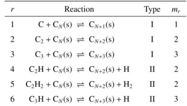
Table 1. Considered chemical surface reactions.
r Reaction Type mr
1 C+CN(s) CN+1(s) I 1
2 C2+CN(s) CN+2(s) I 2
3 C3+CN(s) CN+3(s) I 3
4 C2H+CN(s) CN+2(s)+H II 2
5 C2H2+CN(s) CN+2(s)+H2 II 2
6 C3H+CN(s) CN+3(s)+H II 3
K, Ti) and 150 molecules in our chemical equilibrium code with equilibrium constants newly fitted to the electronic data of the J
tables (Chase et al. 1985). The total carbon abun-dance0C is a free parameter.
For the calculation of the nucleation rate Jwe assume
ho-mogeneous nucleation of pure carbon clusters CNand apply the
modified classical nucleation theory2 according to Gail et al. (1984). All molecules and clusters are assumed to be in LTE with the gas phase. Consequently, the nucleation rate is calcu-lated according to Tg. Besides the directly involved small car-bon clusters C, C2 and C3, the nucleation rate depends on the concentration of some additional small hydrocarbon molecules which contribute to the growth of the carbon clusters
J=J
Tg,nC,nC2,nC2H,nC2H2,nC3,nC3H
. (8)
The net growth of all dust particles included in the dust mo-ments (a≥a) is described by a size-independent growth time
scale
τ−1 gr = τ−gr1
Tg,Td,nC,nC2,nC2H,nC2H2,nC3,nC3H
= 4πa20
r
nrvrelr mrαr
1− 1
bth
r Smr
· (9)
nris the density of the impinging gas particle which initiates
the reaction r,αr is the sticking coefficient and mrthe number
of monomers (carbon atoms) added to the solid surface per re-action. For further definitions and explanations please consult Gail et al. (1984), Gail & Sedlmayr (1988) and Gauger et al. (1990).
The last factor in Eq. (9) accounts for the reverse (evapora-tion) reactions by applying Milne relations with respect to the detailed balance
S = nCkTg pvap(Td)
, where (10)
pvap(T ) = 106dyn/cm2×exp
∆G(T ) RT
, (11)
∆G(T ) = +1.01428×10⁶/T −7.23043×10⁵ +1.63039×10²×T−1.75890×10⁻³×T2
S is the supersaturation ratio which expresses the phase
non-equilibrium between gas and dust, and pvap is the saturation vapour pressure of graphite.∆G is the difference in Gibbs free energy between a solid unit and the monomer in the gas phase, newly fitted according to the J
tables (Chase et al. 1985) in units of [J/mol], and R = 8.31441 J mol−1K−1 is the ideal gas constant. The thermal b-factors bthr express departures from
thermal equilibrium between gas and dust, i.e. TdTg(Gauger et al. 1990; Patzer et al. 1998; Woitke 1999).
Equation (9) allows a generalisation of the definition of the thermal stability of dust grains by means ofτ−1
gr =0. This con-dition states an implicit equation for the determination of one of the arguments ofτgr, which are (utilising Eq. (7)) Tg,Td,nH andCConsequently, the sublimation temperature TSof a dust grain material can be defined as the dust temperature Tdwhich nullifies Eq. (9), i.e.τ−gr1(Tg,TS,nH, C)=0. In thermal equi-librium (where Td=Tgand hence bthr =1), this coincides with
the usual definition of phase equilibrium (S =1). However, in thermal non-equilibrium the criterion is more complicated and the resulting sublimation temperatures depend on the chemi-cal composition of the gas as well as on the considered set of surface reactions.
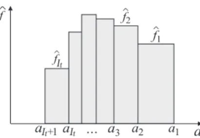
2.3. Discrete dust size distribution function
The dust size distribution functionf (a,r,t) is the basis for the
opacity calculation via Mie theory (see Sect. 2.4). Furthermore, the modelling of the evaporation in the moment method re-quires the knowledge about the dust size distribution func-tion at the lower integrafunc-tion boundary f (a,r,t). We follow
the computational method of Krüger et al. (1995) to obtain the discrete size distribution fi(i=1, ... ,It) on a co-moving
grid in size space with sampling points ai(t) (i=1, ... ,It+1),
where It is the number of grid points at time t, as illustrated
in Fig. 1. Since the growth/shrink rate da/dt is independent of a (Dominik et al. 1989), the evolution of the size distribu-tion funcdistribu-tion during the time interval∆t can be obtained by
shifting the size grid points uniquely by
ai(t+∆t) = ai(t)+
da dt
t×∆t (i=1, ... ,It+1) (13)
da dt
t = a0 3τgr(t)·
(14) The discrete size distribution function is adapted to the evo-lution of nucleation, growth and evaporation according to the following numerical scheme
J(a,t)>0 ⇒generate new grid point:
It+∆t = It+1
aIt+1(t+∆t)=a
fIt = J(a ,t)
da dt t −1
aIt <a ⇒discard grid point:
It+∆t = It−1.
The value of fIt (see l.h.s. interval in Fig. 1) is obtained by
in-tegrating the incoming flux of clusters in size space over ∆t
Fig. 1. Numerical representation of the discrete size distribution function.
through the boundary a = a, assuming thatτgrandJ(a ) are constant within the time step∆t. Only a few more special cases
must be considered for this simple scheme of a discrete rep-resentation of the dust size distribution function, e.g. when no dust is yet present or when the last size bin is to be removed. In these cases, two new grid points must be generated/discarded.
The dust moments can alternatively be calculated by
Kj(t)=
1 (a)j( j+1)
It
i=1
fi
ai
j+1 −ai+1
j+1
(15)
which allows a cross-check with the results obtained from the numerical integration of the moment equations, where
f (a,t)=
fIt,aIt+1≤a
0 ,otherwise. (16)
2.4. Opacity calculations
The gas is assumed to be optically thin in the considered volume and, consequently, gas opacities are neglected in this model. The dust opacities – in particular the dust extinction and angle-integrated scattering coefficients,κext
λ (r,t) andκλsca(r,t),
the albedoγλ(r,t)=κλsca/κλextand the phase functiongλ(ϑ,r,t)
(for definition see Niccolini et al. 2003) – can be computed by applying Mie theory on the basis of the calculated dust size dis-tribution function f (a,r,t), if the optical constants of the dust
material are known (Bohren & Huffman 1983).
It soon became clear, however, that using exact Mie the-ory in each spatial cell of the model volume (see Appendix A) at every time step according to the calculated dust size dis-tribution function would cost too much computing time. We were therefore forced to use an approximate procedure instead. Noting that the dust particles remain quite small in our model (a<0.1µm) the small particle limit of Mie theory (Rayleigh limit) can be considered, whereκλext ∝ K3 (Gail & Sedlmayr 1987). Therefore, as a simplifying approach, we use scaled ex-tinction coefficients according to
κext
λ (r,t)=
K3(r,t)
K3
×κext
λ · (17)
κext
carbon (real and imaginary part of the refractory index) from Rouleau & Martin (1991) to calculateκext
λ ,γλandgλ(ϑ). As a
further simplifying assumption, the albedo and the phase func-tion are not scaled at all, i.e.γλ(r,t) = γλ andgλ(ϑ,r,t) = gλ(ϑ). These relative quantities have little influence on the
resulting temperature structure. We have checked that the tem-perature differences between taking the true Mie opacities and our approximate opacities are less than 5% throughout the model volume3.
2.5. Radiative transfer
The axisymmetric continuum radiative transfer problem is solved at each time step by applying our Monte Carlo method (Niccolini et al. 2003), which assumes time-independence, LTE, angle-dependent coherent scattering and radiative equilibrium.
Several basic improvements of the standard Monte Carlo procedure have been introduced in order to reduce the Monte Carlo noise in the temperature determination and so to en-hance the computational performance of the method. Stellar and cell photon packages are systematically generated and in-dependently propagated through the dust envelope. The dust particles are assumed to be in radiative equilibrium,
κabs
λ Jλdλ=
κabs
λ Bλ(Td) dλ, (18) whereκabs
λ = κλext(1−γλ) is the dust absorption coefficient
and Bλthe Planck function. For each cell, the dust photons are
generated with an initial guess for Td(r,t). Taking advantage of the explicit temperature-independence of the dust opacities, the correct temperature stratification, which satisfies Eq. (18) in every cell, is found by iteration after the Monte Carlo ex-periment has been completed, by applying aΛ-operator tech-nique. This high-precision temperature determination scheme is based on the calculation of mean intensities Jλaccording to the computed path lengths of the photon packages through the cells (Lucy 1999), which gives accurate results for Td(r,t) also in optically thin situations. For further details of this radiative transfer method see (Niccolini et al. 2003, method 1).
As inner boundary condition for the radiative transfer prob-lem, a black body sphere with constant radius Rand constant effective temperature Teff is assumed, which fixes the bolo-metric luminosity L =4πR2σTe4ff. A varying stellar
temper-ature T(t) is introduced to determine the outgoing flux and
the wavelength distribution of the stellar photons. As the dust forms and the optical depths in the model volume increase, photons that are thermally re-emitted or scattered back from the dust shell have a certain probability of hitting the star, which causes an inward directed photon flux at r = R (a radiative
heating of the star) which must be compensated for by an in-crease of the outgoing flux, i.e. T(t)≥Teff. The stellar temper-ature T(t) is initially set equal to Teff, but is part of the afore-mentioned iteration procedure. Incident radiation at the outer boundary is neglected.
3 However, it must be noted that strictly speakingκsca
λ ∝K6in the Rayleigh limit.
The method is suitable for discontinuous opacity struc-tures, such as clumpy media, and is applicable in a broad range of optical depths. For the model under consideration, we use altogether 5 ×10⁷ stellar and 5 ×10⁷ cell photon packages on 30 wavelengths points, covering 0.1µm...250µm, which results in a mean Monte Carlo temperature noise of ∆MCTd ≈ 0.5 K. The Monte Carlo temperature noise ∆MCTd has been estimated by (i) picking a representative K3 (r)-structure from the model and smearing it out over angleθ(see Appendix A), which results in a spherically symmetric dust dis-tribution; (ii) performing a full Monte Carlo radiative transfer calculation; (iii) calculating the standard deviation of the cal-culated temperatures Td(r, θ) at constant radii r; and (iv) taking the mean value of these standard deviations over all radial grid points. One radiative transfer calculation takes about 3.5 min on a Cray T3E-1200 parallel super-computer using 200 pro-cessors. In comparison, the integration of the dust moment equations (Eq. (3)) and the calculation of the size distribution function (Eq. (13)) is computationally cheap, consuming only about 10% of the total computational time.
Concerning the determination of the gas tempera-tures Tg(r,t), we have no access to detailed molecular opaci-ties in our program. Therefore, for simplicity we assume that the gas temperature is given by the black body temperature
Tg(r,t)=Tbb(r,t) defined by
Jλdλ=
Bλ(Tbb) dλ. (19)
2.6. Iteration, initial values and time step control
The model is calculated forward in time by a simple explicit iteration scheme. As initial values at t=0 we choose the dust-free case
f (a,r,t=0)=0 ⇔ Kj(r,t=0)=0. (20)
The iteration starts by calculating the opacities according to the actual values of K3(r,t) (see Sect. 2.4). Based on these opac-ities, e.g. κext
λ (r,t), a complete Monte Carlo radiative
trans-fer calculation including temperature iteration is carried out (see Sect. 2.5), which provides the temperature structure of the medium at time t: Tg(r,t) and Td(r,t).
Next, the dust moment equations are integrated forward for a time step∆t as described in Sect. 2.2, which results in the
dust moments Kj(r,t+ ∆t). This integration is performed on
the assumption that the temperatures Tg(r,t) and Td(r,t) are constant during t∈[t,t+ ∆t].
The moment equations are numerically integrated sepa-rately for each cell (see Appendix A). An internal time step control is necessary to allow for rapid changes of the dust quantities during∆t and so to account for the stiff behaviour of the dust component close to the sublimation temperature. The carbon abundanceC(r,t), the concentrations of the chem-ical species nk(r,t) and the discrete size distributionf (a,r,t)
this occurs after 150−300 time steps, which requires altogether 2−3 eight-hour-jobs on the Cray T3E-1200 parallel super-computer using 200 processors.
The choice of the time step∆t is adapted to the physical
situation at time t in order to ensure that Tg(r,t) and Td(r,t) in fact remain approximately constant during t ∈ [t,t+ ∆t].
We achieve this goal by combining several time scale criteria. Most importantly, K3 must not change too much during∆t in any cell, which would result in a relevant opacity-change that might influence the temperature structure. The maximum al-lowed change of K3during∆t is limited by introducing an abso-lute tolerance (2×10⁻³[0
C−O]) and a relative tolerance (5%).
3. Results
The results obtained from our axisymmetric model calculations are presented in the following way. We show one exemplary model and explain the main physical processes in Sect. 3.1. The radial development of the dust (angle-averaged), is further described in Sect. 3.2 and the angular deviations from the mean values (structure formation) in Sect. 3.3. Section 3.4 gives more insight into the nature of the radiative/thermal instability and discusses where the dust-forming gas in an AGB star wind might be affected by this instability. The functional dependen-cies of the introduced parameters are outlined in Sect. 3.5, and Sect. 3.6 discusses the influence of the forming dust clumps on the spectral appearance of the star by means of calculated spectral energy distributions and monochromatic images.
3.1. A sample model
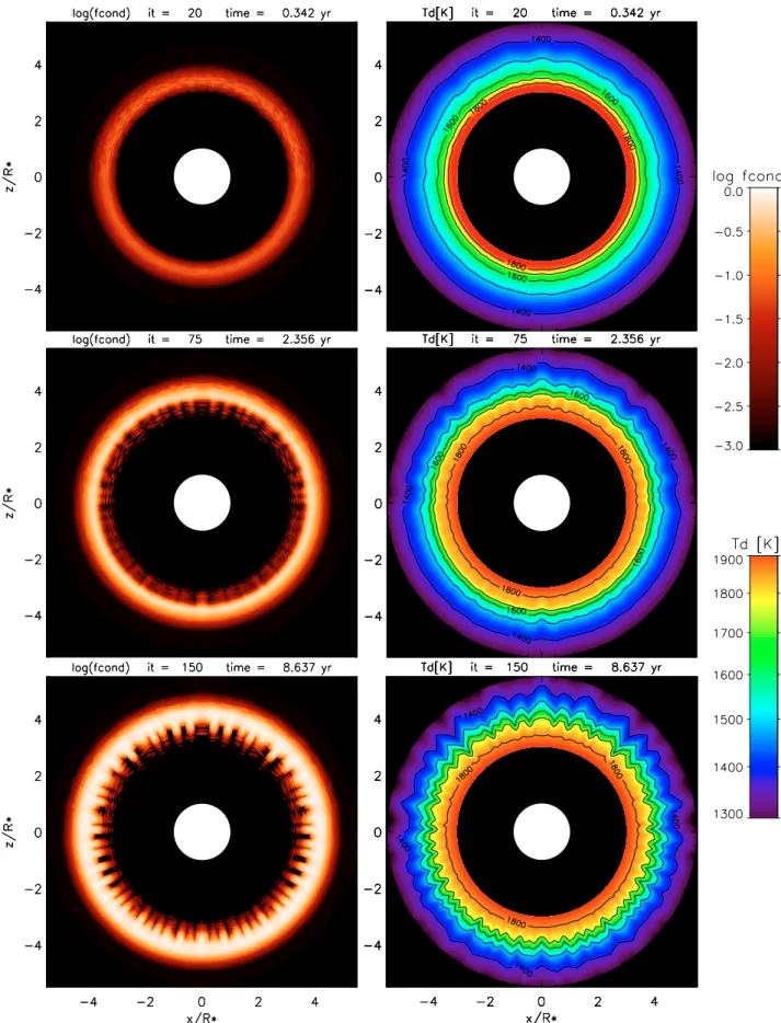
The development of the forming dust shell in a sample model is presented in Fig. 2, showing the degree of conden-sation fcond(r,t) and the dust temperature Td(r,t). The denser
regions close to the star condense first, because the nucle-ation and growth of the dust particles proceed faster at larger densities. Consequently, the spatial dust distribution at first resembles the slightly inhomogeneous gas distribution in the circumstellar shell with a cutoffat the inner edge as a conse-quence of the temperatures being too high for nucleation close to the star, and a smooth outer boundary because of the radi-ally decreasing density. According to the different choices of the density inhomogeneities above and below mid-plane (see Eq. (A.6)), the resulting spatial variations in the degree of con-densation, ∆θlog fcond, are larger above than below the mid-plane at early phases of the model (see upper left plot in Fig. 2). Note that∆θlog fcondis larger than∆θlog nH, because the in-verse dust formation time scale initially scales with the density to the power of 3 to 4 (Woitke 2001).
The process of dust formation continues for a while in this way, until the first cells close to the star become optically thick. Each optically thick cell casts a shadow onto the circumstellar envelope in which the temperatures decrease by several 100 K, which improves the conditions for subsequent dust formation in these shadows. At the same time, scattering and re-emission from the cells that have already condensed intensifies the ra-diation field in between. The stellar flux finally escapes pref-erentially through the segments which are still optically thin,
thereby heating them up and worsening the conditions for fur-ther dust formation fur-there. These two opposing effects amplify the initial spatial contrast of the degree of condensation in-troduced by the assumed density inhomogeneities. In the end, radially aligned, cool, linear dust structures, henceforth called
dust fingers have developed, which point towards the star and
are surrounded by warmer, almost dust-free regions at the inner edge of the forming dust shell. The length of the fingers is of the order of 0.5 R.
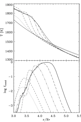
3.2. The chemical wave
Apart from the self-organisation of the dust in the angular di-rection (a second-order effect), the model shows in first or-der the formation and evolution of a radial dust shell. For a better visualisation of these processes, we have plotted sev-eral angle-averaged quantities Xθ(r,t) in Fig. 3. The eff
ec-tive formation of dust generally requires a suitable combina-tion of gas density and temperature, called the dust formacombina-tion
window (Gail & Sedlmayr 1998). Initially, favourable
temper-ature conditions for efficient nucleation are only present in a restricted radial zone close to the star. However, as time passes, the dust shell becomes optically thick which dams the outflow-ing radiation and leads to an increase of the temperatures in-side the shell (radiative backwarming). Consequently, the zone of effective dust formation shifts outward with increasing time. Moreover, the temperatures at the inner edge of the shell tem-porarily exceed the sublimation temperature TS, and the dust shell begins to re-evaporate from the inside. The upper plot of Fig. 3 shows that Tdtemporarily exceeds its equilibrium value which is reached at later stages (see Sect. 3.4).
These two effects result in an apparent motion of the dust shell, driven by dust formation at the outer edge and dust evap-oration at the inner edge of the shell. This wave-like propaga-tion of a dust-formapropaga-tion front will be denoted in the following as chemical wave, since it is solely based on chemical and ra-diative processes without bulk velocity fields (u=0). Chemical waves are a well-known phenomenon in the laboratory, for ex-ample in reaction-diffusion systems, where front-like solutions of the chemical concentrations may exist, sometimes radia-tively controlled (e.g. Schebesch & Engel 1999).
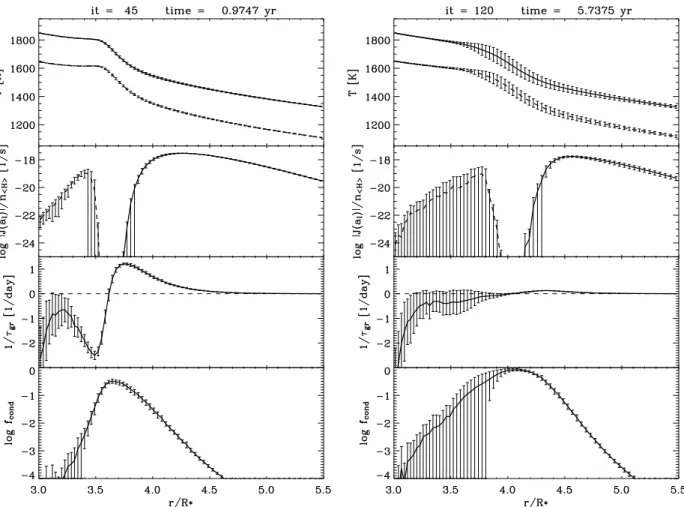
We are interested in these chemical waves, because dust formation is known to happen event-like in these envelopes, e.g. it occurs again and again from scratch, possibly accom-panied by these chemical waves. The apparent propagation velocity of our chemical wave, as determined from Fig. 3, decreases from ≈2 km s−1 (early phase) to ≈0.1 km s−1 (late phase). Figure 4 shows more details of the structure of the chemical wave. The outer regions ahead of the wave feature a positive nucleation rate J(a)=J>0 and a positive growth
time scaleτgr > 0. In the centre of the wave, fcond is maxi-mum and J(a) and 1/τgrvanish. The layers behind the wave (close to the star) usually possess a negative flux through the size integration boundary J(a)<0 and a negative growth time
scaleτgr<0.
Fig. 3. The chemical wave: formation and propagation of a dust shell via dust formation at the outer edge and dust evaporation at the in-ner edge. The figure shows the time evolution of the angle-averaged dust temperature Tdθ(r) (upper plot) and degree of condensation
fcondθ(r) (lower plot). The quantities are shown for iteration step
it=0 (t=0, full), it=10 (t=0.21 yr, dotted), it=20 (t=0.36 yr, dashed), it = 40 (t = 0.84 yr, dashed-dotted), it = 70 (t = 2.1 yr, dashed-triple-dotted), it = 120 (t = 5.7 yr, long-dashed) and it = 195 (t=13 yr, full).
the temperature structure of the medium are mutually cou-pled in a fine-tuned way. This equilibrium is enforced by a
self-regulation mechanism: More dust causes an increase of
the temperature in the neighbourhood via backwarming, which leads again to dust evaporation and vice versa. This mechanism results in a physical state close to phase equilibrium Td →TS (or, alternatively speaking, τgr → ∞, see Sect. 2.2) for long times after the chemical wave has passed, featured by a steep increase of fcondθ(r) and a moderate decrease of Tgθ(r) with increasing r in the wake of the front. The re-laxation time scale towards this equilibrium state is given ap-proximately by the characteristic dust growth/evaporation time scale, |K3/(dK3/dt)|, which is of chemical type and hence density-dependent. As we are limited by our explicit numerical iteration scheme, we are forced to keep the computational time step∆t smaller than this characteristic time scale in the inner
regions (see Sect. 2.6) which makes it computationally difficult to trace the chemical wave much further out, where the dust formation proceeds more slowly by orders of magnitude due to the lower densities.
3.3. Structure formation
Beside the main evolution of the dust component in the
r-direction, the model shows growing inhomogeneities
(struc-ture formation) after the passage of the chemical wave. We vi-sualise these spatial deviations from the angle-averaged values by means of standard variations (∆θX)(r,t) in Fig. 4. These
“er-ror bars” have nothing to do with real “er“er-rors” here, but just give an impression of the magnitudes of the angular variations occurring in the model (compare Fig. 2).
In general, the chemical wave is found to leave behind a strongly inhomogeneous dust distribution, where fcond varies between zero and specific maximum values, which depend on the gas density and the distance to the star. From Fig. 4 (r.h.s.) we see that usually ∆θX(r) > Xθ(r), where X ∈
{J(a),1/τgr,fcond}, for a long time after the passage of the chemical wave in the regions close to the star, i.e. the angu-lar variations of all relevant dust quantities are usually angu-larger than their mean values. This result is a consequence of several factors.
1. The dust formation process requires the formation of seed particles (nucleation), which depends exponentially on Tg
above a certain threshold temperature. Therefore, small
temperature variations may result in large variations of the dust quantities.
2. The dust growth rate is density-dependent. Small density variations temporarily lead to large contrasts of fcond in early phases of the condensation process.
3. The sublimation temperature TS depends on the density. Denser regions are more resistant against thermal evapo-ration, because the partial pressures of carbon molecules in the gas phase are higher and hence the supersaturation ratio S is larger for higher gas densities.
4. Radiative transfer effects introduce a non-local spatial
cou-pling. In particular, dense cells with high fcond cast shad-ows. In the shadowed regions behind these “clouds”, the conditions for the subsequent formation (nucleation) and the survival of the dust (thermal stability) are improved due to shielding effects.
The first two points lead to an inhomogeneous dust distribu-tion already during the early phases of the dust condensadistribu-tion process. As soon as the dust shell becomes optically thick, the backwarming enforces a partial re-evaporation of the dust close to the star, until the radiative energy finds ways to partly es-cape the system. Because of the threshold-like temperature-dependence of the dust survival and the density-temperature-dependence of TS, the dust in the slightly denser cells close to the star can just survive, whereas the dust in the adjacent (slightly thin-ner) cells must evaporate completely. Figure 4 shows that 1/τgr (zero indicates phase equilibrium) varies from slightly positive to considerable negative values behind the chemical wave, i.e. these regions consist of a mixture of cells where the dust is just thermally stable and cells where all dust particles evaporate or have evaporated.
Fig. 4. Detailed radial snapshots of various angle-averaged quantities. Upper row: dust temperatureTdθ(full line) and gas temperatureTgθ
(dashed). Second row: positive nucleation rateJ/nHθ(full line) and negative evaporation rate−J(a)/nHθ(dashed). Third row: inverse
growth time scale1/τgrθ. Lower row: degree of condensationfcondθ. The error bars do not represent errors but standard deviations∆θX of the angular variations of the calculated quantities X(r,t).
the survival of the dust in the shadow of this cell. Therefore, the final equilibrium state of the medium can in fact possess a non-trivial spatial structure, where cool, optically thick seg-ments coexist with warmer, optically thin segseg-ments. The radia-tive flux finally escapes preferentially through these optically thin segments where the degree of condensation remains low (see upper right plot of Fig. 4). Thus, finger-like dust structures develop (see Fig. 2) which point toward the star.
3.4. The metastable region
The driving mechanism for the structure formation is an unsta-ble physical control loop, as discussed exhaustively in Paper I and once again sketched in the upper part of Fig. 5. The physi-cal feedbacks [1] and [3] (temperature-dependence on radiation field and opacity-increase in case of condensation) are always positive and active. However, the feedback [2] diminishes for too low temperatures: Let f◦cond(r) and
◦
T (r) denote the degree
of condensation and the dust temperature structure in the final equilibrium state reached long after the passage of the chemical wave. The ability of the medium to condense can then be ex-pressed byf◦cond(T ). At too low temperatures (large r), a small temperature changeδT , e.g. by shadow casting, has only little
influence on this quantity (as indicated by the vertical arrows in Fig. 5), the control loop is broken and an outer boundary of the metastable region results (see lower part of Fig. 5). On the other hand, the feedback [4] (the non-local effect of opacity on the temperature structure, in particular shadow casting) re-quires that the medium is not completely optically thin, which creates an inner boundary of the metastable region. Here the achievable degree of condensation is too small because of too high temperatures, and since gas opacities are unimportant, the medium cannot attain a considerable optical thickness.
Consequently, significant structure formation only occurs in a limited spatial zone of the model (see Fig. 2) between two boundaries, denoted by [4] and [2] in Fig. 5, henceforth called the metastable region. Here, the matter finally remains in a metastable state which is not fully condensed nor completely dust-free, where small fluctuations cause large effects.
From the numerical results we infer that the size of this
metastable region is essential for the significance of the
form-ing dust structures. Only if this region is large, there is enough space for the radiative/thermal instability to produce well-grown spatial dust structures.
Fig. 5. Sketch of the radiative/thermal instability of dust formation and related size of the metastable region.
of the dust grain material pvap
Td(r)
is given. Note that the
Td-gradient is much smaller inside an optically thick dust shell than in the optically thin case. If the gas density decreases out-ward with a similar gradient, the supersaturation ratio S is of the order of unity in an extended radial zone.
3.5. Functional dependence on model parameters
This paragraph describes the influence of the model parame-ters on the structure formation process, based on the experience gained from other model calculations with different parameters not shown in detail in this paper4. The numbers in square brack-ets in the item list below are the parameter values of the sample model discussed above (in Figs. 2−4).
Teff [3600 K]: the effective temperature of the star determines
the mean radial distance of the dust formation zone. If Teff is
decreased, the metastable zone (see Sect. 3.4) is located closer to the star and results to be narrower, which leads to the forma-tion of less significant dust structures.
nH(r0) [3.7×1010cm−3]: the gas density in the circumstellar environment is responsible for the dust growth time scale and, hence, for the velocity of the chemical wave. If this parame-ter is changed, the model shows basically the same behaviour, but all processes occur on a different time scale. Furthermore, larger densities lead to an increase of TS, which means that the formation and the survival of dust are possible closer to 4 See mpeg-movies at http://astro.physik.tu-berlin.de/
∼woitke/sfb555.html
the star, and larger densities potentially lead to the formation of more dust, which produces larger optical depths. In models with strongly reduced nH(r0), the resulting optical depths are too small to cause significant temperature changes via back-warming and shadow casting, and the system decouples spa-tially, i.e. every cell condenses on its own, without much effect on their neighbourhood. In models with larger nH(r0), we ob-serve that only slightly larger optical depths occur than in the sample model, but that the dust shell is narrower. This is a con-sequence of the re-evaporation process which sets in as soon as a certain critical value ofτ1µmis reached (here about 1...3). The temperatures temporarily reach higher values behind the wave as depicted in Fig. 3 and the dust evaporation is faster and more complete on the inside of the shell. In both cases of varied nH(r0), less pronounced structure formation is found to occur.
C/O [2.0]: the initial carbon-to-oxygen ratio is a measure of the amount of condensable material in the gas. Consequently, changing C/O has a similar influence as changing the overall density level (nH(r0)).
Hρ [0.25 R]: the scale height is important for the radial
ex-tension of the metastable zone (see Sect. 3.4). We observe from models with larger Hρ that the size of the metastable zone is
smaller and, consequently, the structure formation is less sig-nificant. However, even for models with nH ∝ 1/r2, where the density gradient is much shallower, some structures still develop.
C2 [0.1/0.03]: the degree of density inhomogeneities (see Eq. (A.4)) is not a critical parameter of the model! From Fig. 2 we see that in the end the number and the shape of the dust structures is similar above and below the mid-plane, despite the different values for C2. The finger-like structures even develop for C2 =0. For larger density inhomogeneities, the structures become slightly longer and less numerous.
Spatial resolution [71×71grid points]: the number of radial grid points in the model is important for the proper resolution of the radiative transfer and the propagation velocity of the chem-ical wave. The number of angular grid points is crucial with respect to the shape and, in particular, the width of the result-ing dust structures. In the depicted model (Fig. 2), Nstruc =27 dust structures can be identified within Nθ+1=71 angular grid
points, i.e. the resulting number and width of the dust fingers is at the limit of the angular resolution of the model.
The resulting width of the dust fingers is possibly a conse-quence of the way in which we have introduced the density inhomogeneities in our model. Since we use for all cells inde-pendent random numbers (see Appendix A), the resulting den-sity inhomogeneities are spatially uncorrelated and the charac-teristic scale of the density variations is naturally given by the size of the cells, which is apparently important for the width of the dust fingers. We have run model calculations with up to 181 angular grid points (which forces us to reduce Nrto 40
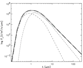
Fig. 6. Calculated spectral energy distribution of the clumpy model at
t = 13.2 yr, averaged over all escape directions. Flux values corre-spond to a distance of 1 R. Full line: calculated total flux, dotted line:
direct star light, thin dashed line: scattered star light, dashed-dotted line: thermal dust emission (partly scattered), thick grey dashed line: total flux of a spherically symmetric reference model (see text).
The ratio Nstruc/Nθbecomes lower if Nθis increased. However,
definite predictions about the diameter of the dust structures are difficult to make, because of the limited angular resolution in our model. Because of computational restrictions, we cannot decide whether an asymptotic limit for Nstrucexists (or possibly for Nstruc/Nθ) for Nθ→ ∞.
3.6. Spectral appearance
From an observational point of view it is interesting to dis-cuss how a “clumpy” dust distribution around an AGB star would appear both spectroscopically and in monochromatic images. Figure 6 shows the calculated spectral energy distri-bution (SED) of the sample model at the end of the computa-tion. The depicted flux has been averaged over all escape di-rectionsθesc, φesc(see Niccolini et al. 2003). The resulting SED is featureless according to the amorphous carbon opacities and can reasonably well be fitted by a black body with colour tem-perature≈2700 K...2900 K (note the difference to the effective temperature Teff=3600 K).
The Monte Carlo method allows an identification of the kind of photons which reach the observer. The optical (blue) part of the spectrum mainly results from direct star light, which is attenuated by dust extinction, and from multiply scattered star light. The near IR spectral region around 2µm...4µm is dominated by thermal dust emission, whereas for longer wave-lengths the dust envelope becomes optically thin and the direct star light again becomes the most important contributor (which is an artifact of our model, because it is radially not sufficiently extended).
To our surprise, the angle-averaged SED contains almost no evidence of the clumpy dust distribution in the model, contrary to the results from simplified models for spectral analysis (e.g. Jørgensen et al. 2000). We have calculated a time-dependent
Table 2. Comparison of the “clumpy” sample model to a spherically symmetric reference model at t = 13.2 yr (see text).TdMd is the
mass-averaged dust temperature andτ1µmthe radial optical depth at
λ=1µm.
Clumpy model Reference model
Mgas[M] 1.35×10⁻⁶ 1.35×10⁻⁶
Mdust[M] 5.23×10⁻¹⁰ 4.69×10⁻¹⁰
τ1µm 0.51. . .2.7 0.98
T[K] 3610.7 3610.6
TdMd[K] 1638 1654
reference model which is identical to the sample model, ex-cept for the choice of Nθ =1, i.e. all “cells” are closed
spher-ical shells in the reference model, which enforces the results to be spherically symmetric. Figure 6 shows that the angle-averaged SED of the “clumpy” model is practically indistin-guishable from the SED of the spherically symmetric reference model at a comparable instant of time. There is only a slight ex-cess in the blue part of the spectrum compared to the reference model (e.g.+15% atλ=0.34µm,+4% atλ=0.55µm,+1% atλ=0.72µm), caused by the increased escape probability in the blue in case of a clumpy medium.
Table 2 gives more details of this comparison. In fact, about 10% more dust (by mass) condenses in the clumpy model than in the spherically symmetric reference model. The stan-dard deviation of the optical depth atλ = 1µm is larger than its mean value τ1µm. The mass-averaged dust temperature TdMd = ξVξn
ξ
HK
ξ
3 T
ξ
d ξVξn
ξ
HK
ξ
3
is slightly lower than in the reference model, where Vξ is the volume of cellξ. In summary, if the assumption of spherical symmetry is relaxed to axisymmetry, more dust condenses in the stellar environment which forms and survives in radiatively shielded, cool clumps, resulting in a lower mean dust temperature. However, the char-acteristic changes are only of the order of 10%, and it is note-worthy that the different single effects tend to compensate each other concerning the total effect on the spectral appearance of the star.
From Fig. 6, we can infer that the spectral region around 2µm...4µm, which approximately coincides with the maxi-mum of the thermal emission from the dust envelope, is most promising for revealing the spatial dust distribution around the star by direct imaging. Figure 7 shows simulated pictures at
λ = 2.2µm. The light from the dust shell mainly arises from the glowing heads of the dust fingers, which appear as rings around the star because of our assumption of axisymmetry. The different physical contributions are shown separately in Fig. 7. However, the intensities received from the dust shell are about one order of magnitude less than the intensities received from the star. The lower right image depicts the total brightness distribution, where basically only a stellar disk is visible, which is partly obscured by the inhomogeneous dust distribution around the star.
direct dust emission
scattered dust emission
scattered star light
total
Fig. 7. Simulated images of the innermost±4.5 Rof the model at 2.2µm for an inclination angle of 20◦between the equator and the line of
sight. The dust distribution refers to the final state of the model (t=18.4 yr). The total signal is shown in the lower right plot, whereas the other (artificial) images show the different constituents of the signal (total=direct star light+scattered star light+direct dust emission+scattered dust emission). Note the different scaling of the intensities, given in units of 10 W m−2µm−1for a reference distance of 1 R
. The picture of the
(Lynds et al. 1976; Gilliland & Dupree 1990). However, an inhomogeneous dust distribution around the star (which is a perfectly uniform black body sphere in our model) can ob-viously lead to a similar optical appearance, even if there is not much direct evidence for dust in the image. On the ba-sis of only one observational image, it seems actually diffi -cult to decide which physical interpretation is correct (sur-face convection/non-uniform dust formation). Multi-epoch, or even better simultaneous multi-wavelength images would be required to come to definite conclusions, since surface convec-tion and dust formaconvec-tion may occur on similar time scales. Thus, the interpretation of monochromatic images, e.g. by speckle interferometry, via cool and hot spots on the stellar surface is delicate if there is only very slight evidence for the existence of circumstellar matter, e.g. by spectroscopy, which could be inhomogeneous.
In fact, the direct+scattered star light only pro-vides≈40%+8% of the total signal integrated over the entire image, whereas≈37%+15% originates from the dust enve-lope (direct+scattered dust emission). However, the dust emis-sion is spread over a much more extended area, here∼π(4 R)2,
than the direct star light∼πR2
. Consequently, the intensities
re-ceived from the dust envelope are generally much weaker than the intensities received from the stellar disk (factor∼16).
The different physical contributions to the image are sep-arately shown in Fig. 7. A composite picture of scattered star light+direct dust emission+scattered dust emission (lower left+upper left+upper right in Fig. 7) would simulate a coro-nagraphic image where the stellar disk is blinded out. Such observations could in fact reveal the spatial dust distribution around the star. Of course, since our model is axisymmetric, the “clumpy” dust distribution in the model appears as super-position of rings in the image, and this is not expected to be realistic. Nevertheless, the images give a first impression of the kind of brightness distributions to be expected from a cloudy circumstellar environment.
4. Conclusions and discussion
We have shown in this paper that the formation of dust shells in the circumstellar environments of late-type stars can be un-stable. Spontaneous symmetry breaking may occur because of a radiative/thermal instability in the dust-forming gas, which leads to the development of cloud-like dust structures close to the star.
These results have been obtained on the basis of time-dependent axisymmetric models, which combine a kinetic de-scription of carbon dust formation/evaporation with detailed, frequency-dependent radiative transfer by means of a Monte Carlo method, in the static case. The simulations show that the dust preferentially forms behind already condensed re-gions, which shield the stellar radiation. In the shadow of these clumps, the temperatures are lower by a few 100 K which trig-gers the subsequent formation and facilitates the survival of dust close to the star. As final result, numerous finger-like dust structures develop which may have a radial extension as large as 0.5 Rand point towards the centre of the radiant emission,
similar to the “cometary knots” observed in planetary nebulae and star formation regions.
The cloudy dust distribution has little effect on the calcu-lated spectral energy distribution of the star, in comparison to a spherically symmetric reference model, but significantly in-fluences the optical appearance of the circumstellar environ-ment in near IR monochromatic images (e.g. atλ=2.2µm). In particular, an inhomogeneous dust distribution in front of the star leads to a likewise non-uniformly bright appearance of the stellar disk, usually interpreted as hot/cool spots on the stellar surface. However, our model shows that a different physical ex-planation by clumpy dust is possible, even if the dust is barely visible elsewhere in the image.
Because of computational restrictions, we have so far only been able to study the static case where velocity fields are ig-nored. In this case, the main feature of the model is the for-mation of a chemical wave which propagates outward radially, driven by dust formation on the outer edge and dust evapora-tion due to backwarming at the inner edge. The optical depth of this chemical wave reaches aboutτ1µm<∼1 to 3 with a density-dependent propagation velocity of≈0.1 km s−1to 2 km s−1. The wave leaves behind a strongly inhomogeneous dust distribution close to the star, where the medium relaxes towards phase equi-librium. However, this process is unstable and results in the aforementioned simultaneous occurrence of cool dusty cally thick) segments next to warmer, almost dust-free (opti-cally thin) segments, through which the radiative flux finally escapes preferentially.
According to dynamical (but spherically symmetric) mod-els of dust-forming AGB stars (e.g. Winters et al. 2000; Schirrmacher et al. 2003; Höfner et al. 2003; Sandin & Höfner 2003), the formation of dust mainly occurs in particular phases of the model triggered by the pulsation of the star, which re-sults in radial dust shells. During such a dust shell formation event, re-evaporation from the inside is a typical feature, sim-ilar to the behaviour of our chemical wave. According to the present paper, this process should be unstable and might result in departures from spherical symmetry.
We believe that this instability can provide a basis for a bet-ter understanding of inhomogeneous dust distributions show-ing up in many observations. However, direct predictions for particular objects are difficult to make, because the current model lacks hydrodynamics. Since the dust is blown away as soon as it forms, the system has only little time to relax to-wards phase equilibrium at the inner edge of the dust shell. On the one hand, this time may be too short to produce well-grown spatial dust structures such as those discussed in this paper. On the other hand, even small deviations from spherical symmetry may trigger important dynamical effects, e.g.
– The radiation pressure on dust grains, which is delivered to the gas via frictional forces, mainly depends on the radia-tive flux and the degree of condensation. If slightly more condensed regions exist, they might be accelerated out-ward, whereas less condensed regions stay behind or even fall back.
the inner edge of the cloud facing the star than at its self-shielded outer edge (this effect does not occur in spherically symmetric models where r2F(r)=const.in radiative equi-librium). Driven, pancake-like structures could evolve due to this effect.
– The hydrodynamical process of cloud acceleration due to radiation pressure is not well-studied, apart from the special case of spherical symmetry. This process may be dynamically unstable itself (e.g. Rayleigh-Taylor, Kelvin-Helmholtz). Velocity disturbances generated by these instabilities may have an important effect on the dust-forming medium.
Thus, we propose a new hypothetical scenario for dust-driven AGB star winds: excited by hydrodynamical, radiative or ther-mal instabilities, dust clouds are formed from time to time close to the star in temporarily shielded areas, which are accelerated outward by radiation pressure. At the same time but at diff er-ent places, thinner, dust-free matter falls back towards the star. A highly dynamical and turbulent environment close to the star would be created in this way, which can be expected to produce again a strongly inhomogeneous dust distribution.
In order to verify this hypothetical scenario, much more elaborate model calculations would be required which may well exceed the present capabilities of parallel super-computers. Various processes must be traced in 3D, using dynamical models with detailed radiative transfer and time-dependent dust chemistry.
Acknowledgements. The authors would like to thank Dr. Christiane Helling for numerous discussions about how to improve the manuscript. This work has been supported by the DFG, Sonderforschungsbereich 555, Komplexe Nichtlineare Prozesse, Teilprojekt B8, and by the DAAD in the PROCOPE program under grant D/9822849 and 99001. The numerical computations were performed on the T3E parallel computer at the Konrad-Zuse-Zentrum für Informationstechnik Berlin, project bvpt17.
Appendix A: Spatial grid
The model volume is subdivided into fixed spatial cells, where the cell boundaries are specified in spherical coordinates r,θ andφ, using prescribed sampling points for the radius and the latitude angle, rnandθk, respectively. A cell is the volume
de-fined by the following coordinate intervals
r∈[rn−1,rn] n=1, ... ,Nr (A.1)
θ∈[θk−1, θk] k=1, ... ,Nθ (A.2)
φ∈[0,2π]. (A.3)
According to Eq. (A.3) the cells are closed tori, i.e. the model is axisymmetric (2D). Each cell is specified by one radial and one angular index, n and k, respectively, which are abbreviated by a multi-indexξ=(n,k). For the model discussed in detail in
this paper, we choose a radial grid with Nr+1=71 logarithmic
equidistant sampling points between r0/R=3.0 and rNr/R=
5.5 and Nθ+1 = 71 equidistant angular grid points between
θ0=0 andθNθ =π. The spatial grid is visualised in Fig. A.1.
Fig. A.1. Spatial grid of the axisymmetric model. Each cell is a torus which appears twice (at x > 0 and x < 0) in this cut through the
y = 0 plane. Blank regions are not included in the model volume (the photons are assumed to pass through these regions). The star is indicated as a central disc.
The prescription of the density structure in the model vol-ume (Eq. (1)) is technically realised in each cellξvia
nξH=C1×exp
−¯rξ
Hρ +C2×Z
, (A.4)
where ¯rξ=(rn−1+rn)/2 the mean radial distance of cellξand Z
a random number with Gaussian distribution and unity variance
Z= −2 ln (1−z1)×sin (2πz2). (A.5)
z1,z2 ∈[0,1) are equally distributed pseudo-random numbers.
C1=6×1015cm−3is a constant chosen to produce the desired mean particle density of hydrogen nuclei at the innermost radial grid point nH(r0). If a continuous stellar wind with ˙M(˜r) = 4π˜r2ρ(˜r)v(˜r) was considered, this choice would be consistent with an outflow velocity ofv(˜r) = 5 km s−1 and a mass loss rate of ˙M(˜r) = 10−7 M/yr at the mean radius of the model volume ˜r = (rNr +r0)/2. In order to study the influence of
the assumed level of density inhomogeneities, we choose the second constant as
C2=
0.10, above mid-plane
0.03, below mid-plane. (A.6)
The standard deviation of the density at constant radius,∆θ×
log nH, is 10%×log e≈4.3% above and 3%×log e ≈1.3% below the mid-plane of the model volume (z=0).
References
Andersen, A. C., Höfner, S., & Gautschy-Loidl, R. 2003, A&A, 400, 981
Bohren, C. F., & Huffman, D. R. 1983, Absorption and Scattering of Light by Small Particles (New York: John Wiley & Sons) Chase Jr., M. W., Davies, C. A., Downey Jr., J. R., et al. 1985, JANAF
Thermochemical Tables, National Bureau of Standards Diamond, P. J., & Kemball, A. J. 2003, ApJ, 599, 1372 Dominik, C., Gail, H.-P., & Sedlmayr, E. 1989, A&A, 223, 227 Feast, M. W., Whitelock, P. A., & Marang, F. 2003, MNRAS, 346,
878
Fleischer, A. J., Gauger, A., & Sedlmayr, E. 1995, A&A, 297, 543 Freytag, B., & Höfner, S. 2003, poster contribution at International
Scientific Meeting of the Astronomische Gesellschaft, September 15−19, 2003, Freiburg, Germany, AG abstract series, 20
Gail, H.-P., & Sedlmayr, E. 1987, A&A, 171, 197 Gail, H.-P., & Sedlmayr, E. 1988, A&A, 206, 153
Gail, H.-P., & Sedlmayr, E. 1998, in Chemistry and physics of molecules and grains in space, Faraday Discussion No. 109, London, GB, 303
Gail, H.-P., Keller, R., & Sedlmayr, E. 1984, A&A, 133, 320 Gauger, A., Gail, H.-P., & Sedlmayr, E. 1990, A&A, 235, 345 Gilliland, R. L., & Dupree, A. K. 1996, ApJ, 463, L29 Haniff, C. A., & Buscher, D. F. 1998, A&A, 334, L5
Heske, A., Te Lintel Hekkert, P., & Maloney, P. 1989, A&A, 218, L5 Höfner, S., Gautschy-Loidl, R., Aringer, B., & Jørgensen, U. G. 2003,
A&A, 399, 589
Jørgensen, U. G., Hron, J., & Loidl, R. 2000, A&A, 356, 253
Jura, M., Chen, C., & Plavchan, P. 2002, ApJ, 569, 964 Krüger, D., Woitke, P., & Sedlmayr, E. 1995, A&AS, 113, 593 Lopez, B. 1999, in AGB stars, ed. T. Le Bertre, A. Lèbre, & C.
Waelkens, IAU Symp., 191, 409 (ASP) Lucy, L. B. 1999, A&A, 345, 211
Lynds, C. R., Worden, S. P., & Harvey, J. W. 1976, ApJ, 207, 174 Monnier, J., Millan-Gabet, R., Tuthill, P., et al. 2004, ApJ, 605, 436 Niccolini, G., Woitke, P., & Lopez, B. 2003, A&A, 399, 703 O’Dell, C. R. 2000, AJ, 119, 2311
Olofsson, H., Bergman, P., Lucas, R., et al. 2000, A&A, 353, 583 Patzer, A. B. C., Gauger, A., & Sedlmayr, E. 1998, A&A, 337, 847 Redman, M., Viti, S., Cau, P., & Williams, D. 2003, MNRAS, 345,
1291
Rouleau, F., & Martin, P. G. 1991, ApJ, 377, 526 Sandin, C., & Höfner, S. 2003, A&A, 404, 789 Schebesch, I., & Engel, H. 1999, Phys. Rev. E, 60, 6429
Schirrmacher, V., Woitke, P., & Sedlmayr, E. 2003, A&A, 404, 267 Schröder, K.-P., Winters, J. M., & Sedlmayr, E. 1999, A&A, 349, 898 Tuthill, P., Monnier, J., Danchi, W., & Lopez, B. 2000, ApJ, 543, 284 Weigelt, G., Balega, Y., Blöcker, T., et al. 1998, A&A, 333, L51 Winters, J. M., Le Bertre, T., Jeong, K. S., Helling, Ch., & Sedlmayr,
E. 2000, A&A, 361, 641
Wiscombe, W. J. 1980, Appl. Opt., 19, 1505
Woitke, P. 1999, in Astronomy with Radioactivities, ed. R. Diehl, & D. Hartmann, MPE Report 274 (Germany: Schlos Ringberg), 163 Woitke, P. 2001, Rev. Mod. Astron., 14, 185