Counting
process-based
dimension
reduction
methods
for
censored
outcomes
ByQIANGSUN
DepartmentofStatisticalSciences,UniversityofToronto,100StGeorgeStreet,Toronto, OntarioM5S3G3,Canada
RUOQINGZHU
DepartmentofStatistics,UniversityofIllinoisatUrbana-Champaign,725SouthWrightStreet, Champaign,Illinois61820,U.S.A.
TAOWANG
DepartmentofBioinformaticsandBiostatistics,ShanghaiJiaoTongUniversity, 800DongchuanRoad,MinhangDistrict,Shanghai200240,China
ANDDONGLINZENG
DepartmentofBiostatistics,UniversityofNorthCarolinaatChapelHill,3101 McGavran-GreenbergHall,ChapelHill,NorthCarolina27599,U.S.A.
Summary
Weproposecountingprocess-baseddimensionreductionmethodsforright-censoredsurvival data. Semiparametricestimatingequationsareconstructedtoestimatethedimensionreduction subspaceforthefailuretimemodel.Ourmethodsaddresstwolimitationsofexistingapproaches. First, usingthe countingprocessformulation, theydo notrequireestimation of thecensoring distributiontocompensateforthebiasinestimatingthedimensionreductionsubspace.Second, the nonparametricestimation involvedadapts tothestructural dimension,soour methods cir-cumventthecurseofdimensionality.Asymptoticnormalityisestablishedfortheestimators.We proposeacomputationallyefficientapproachthatrequiresonlyasingularvaluedecompositionto estimatethedimensionreductionsubspace.Numericalstudiessuggestthatournewapproaches exhibit significantly improved performance. The methods are implemented in the R package orthoDr.
Some keywords: Estimating equation; Semiparametric inference; Sliced inverse regression; Sufficient dimension
1. Introduction
Dimension reduction is important in regression analysis. Its goal is to extract a low-dimensional subspace from ap-dimensional covariateX = (X1,. . .,Xp)Tin order to predict an outcome of
interestT. The dimension reduction literature often assumes the multiple-index model
T =hBTX,, (1)
where is a random error independent of X, B ∈ Rp×d is a coefficient matrix withd < p, andh(·)is an unknown link function. This model is equivalent to assumingT⊥⊥X |BTX (Li, 1991). Since anyd linearly independent vectors in the linear space spanned by the columns of
B also satisfy model (1) for someh, we denote this linear subspace byS(B). The intersection of all subspaces satisfyingT⊥⊥X |BTX is called the central subspace,S
T|X, whose dimension
is referred to as the structural dimension. According toCook(2009),ST|X is uniquely defined
under mild conditions. The goal of sufficient dimension reduction is to determine the structural dimension and the central subspace using data.
There is an extensive literature on estimating the central subspace for completely observed data, includingLi(1991),Cook & Weisberg(1991),Zhu et al.(2006),Li & Wang(2007),Xia
(2007), andMa & Zhu(2012). WhenT is subject to right censoring, model (1) includes many well-known survival models as special cases, such as the proportional hazards model (Cox,1972), the accelerated failure-time model (Lin et al.,1998), and linear transformation models (Zeng & Lin,2007).
There has been limited work on estimating the dimension reduction subspace in the presence of censored observations.Li et al.(1999) propose a modified sliced inverse regression method that uses the estimate of the conditional survival function to account for censored cases. Xia
et al.(2010) propose to estimate the conditional hazard function nonparametrically and use its
gradient to construct the dimension reduction directions. InLi et al.(1999),p-dimensional kernel estimation is used to compensate for the bias caused by censoring, while inXia et al.(2010), the estimation procedure requires ap-dimensional kernel estimate of the hazard function to provide reliable initial values, and then gradually reduces the working dimension to d. These methods suffer from the curse of dimensionality. Whenpis not small, alternative approaches such as that
ofLu & Li(2011) adopt an inverse probability weighting scheme, which implicitly requires the
correct specification of the censoring mechanism.
In this paper, we propose a counting process-based dimension reduction framework that leads to four different approaches. The proposed methods address several limitations of the existing work. First, our framework is built upon a counting process representation of the underlying survival model. This framework allows construction of doubly robust estimating equations, and the resulting estimators are more stable than existing ones such as in Xia et al. (2010). Our formulation can avoid the linearity assumption (Li,1991) and the estimation of any censoring distribution, which are necessary inLi et al.(1999) andLu & Li(2011). Second, the proposed framework is adaptive to the structural dimension in the sense that the nonparametric estimation involved depends only on the dimension ofS(B), which is usually small, thus circumventing the curse of dimensionality. To this end, the proposed method shares advantages similar to that in
Xia et al.(2010). Computationally, we use an optimization technique (Wen & Yin,2013) on the
2. Proposedmethods
2.1. Semiparametricestimatingequationsforthecentralsubspace
Throughout the paper, we denote the failure time by T and the censoring time by C. Let
Y =min(T,C) and δ = I(T C) be the observed event time and the censoring indicator. We assume that C is independent of T conditional on X. Let N(u) = I(Y u,δ = 1) and
Y(u)=I(Yu)denote the observed counting process and the at-risk process, respectively. Let λ(u | X)be the conditional hazard forT givenX. According toXia et al.(2010), model (1) is equivalent toλ(u|X)=λ(u|BTX). Let
dM(u,X)=dM(u,BTX)=dN(u)−λ(u|BTX)Y(u)du
be the martingale increment process indexed byu. This paper considers constructing estimation equations that are based on the counting process representation of the survival model. To derive the estimating equations, we followBickel et al.(1993) andTsiatis(2007) to obtain the ortho-complement of the nuisance tangent space atBas
E⊥= α(u,X)−α∗(u,BTX)dM(u,X): α(u,X)is measurable inX andu , (2)
where α∗(u,BTX) = Eα(u,X) | F u,BTX
and Fu is the filtration; see the Supplementary
Material. To estimateB, we consider the unbiased estimating equations
E α(u,X)−α∗(u,BTX)dN(u)−λ(u|BTX)Y(u)du=0. (3)
The sample versions based onnindependent and identical copies{Yi,δi,Xi}ni=1are
1
n n
i=1
α(u,Xi)−α∗(u,BTXi)
dNi(u)−λ(u|BTXi)Yi(u)du
=0, (4)
where the conditional hazard function will be estimated using data. For some particular choices of α(u,X), this can be implemented using the generalized method of moments
(Hansen,1982):
arg min
B
ψn(B)Tψn(B)
, (5)
where ψn(B) is the vectorized left-hand side of (4). We estimate several quantities in ψn(B)
nonparametrically. For example, the conditional hazard functionλ(u|BTX
i)at any time-pointu
can be estimated by
ˆ
λ(u|BTX =z)= n
i=1Kb(Yi−u)δiKh
BTX i−z
n j=1I
Yj u
Kh
BTX
j −z
(6)
for bandwidthsbandh, whereKh(·)is ad-dimensional multivariate kernel function. We defer
It is crucial to choose specific forms of α(u,X). Different choices may simplify the above formulation or may have theoretical or computational advantages. In the following two subsec-tions, we present four different choices, which fall into two categories: the forward and inverse regression schemes. The main difference between the two schemes lies in whether the counting processN(u)is used in the definition ofα(u,X). The forward regression scheme is essentially the estimating equation approach, while the inverse regression scheme usesN(u)to mimic the sliced inverse regression (Li,1991) conceptually.
2.2. Forward regression
In the forward regression scheme, we chooseα(u,X)to not depend on the observed failure processN(u). Provided thatα(u,X)depends at most on the at-risk processY(u), we can simplify
the estimating equations in (3) to
E
α(u,X)−Eα(u,X)|Y(u)=1,BTXdN(u)
=0.
We now give one example ofα(u,X)when the structural dimensiond =1. This requires only scalar nonparametric estimation.
Example 1. With α(u,X) = X, the population versions of the p-dimensional estimating equations are
E
X −EX |Y(u)=1,BTXdN(u)
=0, (7)
which reduce to the efficient estimating equations for the proportional hazards model when the exponential link is known to be correct. This can also be used for the transformation models in
Zeng & Lin(2007). For some simple extensions, we could letα(u,X)=E{XY(u)}XTto obtain
p-by-p estimating equations, in order to handle the case ofd > 1. To implement the forward regression method in (7), we can estimateψn(B)in (5) using
ˆ
ψn
B= 1 n
n
i=1
Xi− ˆE(X |Y Yi,BTXi)
δi, (8)
where for any givenuandz,
ˆ
E(X |Y u,BTX =z)=
n
i=1XiI
Yi u
Kh
BTX i−z
n i=1I
Yi u
Kh
BTX
i−z
(9)
for some choice of kernel functionKh(·)with bandwidth parameterh; see §3.
2.3. Inverse regression
In this subsection, we focus on the inverse regression scheme. Our motivation is the following counting process representation of the model:
where dN(t)=N(t+dt)−N(t). Hence, we can consider the sliced conditional mean ofX given the outcome of dN(t)in the risk set, that is,Y(t) =1. This leads to the construction of a local mean difference for the binary outcome dN(u):
ϕ(u)=EX |dN(u)=1,Y(u)=1−EX |dN(u)=0,Y(u)=1. (10)
The outcome dN(u)conditioning on the eventY(u)=1 depends only onλ(u|BTX). Hence the
inverse regression curveϕ(u)is contained within the central subspaceST|X. With this choice of
ϕ(u), we consider the function
α(u,X)=XϕT(u). (11)
Then
α(u,X)−α∗(u,BTX)=X −E{X |Y(u)=1,BTX}ϕT(u), (12)
which can be estimated by combining the estimate ofE{X |Y(u)= 1,BTX}in (9) and that of
ϕ(u)in (10):
ˆ
ϕ(u)=
n
i=1XiI
uYi <u+h,δi =1
n i=1I
uYi <u+h,δi =1
−
n
i=1XiI
Yi u
n i=1I
Yi u
. (13)
Based on this choice of α, we propose two approaches that use the estimating equations (3) and a computationally efficient approach that further simplifies the formula to a singular value decomposition.
Example2. Replacingα(u,X)−α∗(u,BTX)in (3) by (12) leads to estimating equations of a
semiparametric inverse regression approach:
E X −E{X |Y(u)=1,BTX}ϕT(u)dM(u)
=0. (14)
This approach consists ofp×pestimating equations, and is able to handle the case ofd > 1. However, the nonparametric estimation part is onlyd-dimensional, as reflected byBTX.
Further-more, this formulation enjoys the double robustness property, illustrated in the Supplementary Material. A similar phenomenon has been observed byMa & Zhu(2012) in the setting without censoring. This suggests that if one ofE{X |Y(u)=1,BTX}andM(u)is estimated incorrectly,
we can still obtain consistent estimators of the dimension reduction subspace. In our numerical experiment, we observe a numerical advantage of this approach over its simplified version, which is given in Example3.
To implement this method, we estimateψn(B)in (5) by
vec
1
n n
i=1
n
j=1
δj=1
Xi− ˆE
X |Y Yj,BTXi
ˆ
ϕT(Y j)
δiI(j=i)− ˆλ
Yj |BTXi , (15)
where Eˆ{X | Y u,BTX = z} and ϕˆT(u) are given in (9) and (13), respectively, and the
Example3. Similar to Example1, our choice ofα(u,X)in (11) depends on at most the at-risk processY(u). Hence, the estimating functions in (14) can be simplified to
E X −E{X |Y(u)=1,BTX}ϕT(u)dN(u)
. (16)
Replacing dM(u)with dN(u)greatly reduces the computational burden. This can be seen from (15), where a conditional hazard functionλˆYj | BTXi
needs to be evaluated at each observed failure time-pointjfor all observationsi. Using this simplification, we lose the double robustness property. The implementation of this approach is a simplified version of that in Example2with
ˆ
ψn
B=vec
1
n n
i=1
Xi− ˆE
X |Y Yi,BTXi
δiϕˆT(Yi)
, (17)
where the estimators of the nonparametric components are the same as before.
Example4. With additional assumptions,Bcan be estimated without nonparametric smooth-ing. We need the following definitions.
Definition1. For anyα ∈ Rpand any u >0, the linearity condition (Li,1991) is satisfied
conditioning on the event{Y(u)=1}, i.e.,
E{αTX |Y(u)=1,BTX =z} =c
0(u)+cT(u)z, (18)
where c0(u)and c(u)are constants that possibly depend on u. Furthermore, the time-invariant
covariance condition requires
cov{X |Y(u)=1} =c1(u), (19)
where c1(u)is some constant depending on u.
After centringX at timeu, if (18) and (19) are satisfied, we have
E{X |Y(u)=1,BTX} −E{X |Y(u)=1} =PX −E{X |Y(u)=1}, (20)
whereP=B(BTB)−1BTand the constant termc
1(u)vanishes. By (19),Premains the same
across all time-points. Hence, inserting (20) into (16) leads to
Q E X −E{X |Y(u)=1}ϕT(u)dN(u)
=0,
whereQ=I −P. This is equivalent to deriving the left-singular space of the covariance matrix
E X −E{X |Y(u)=1}ϕT(u)dN(u)
. (21)
Remark1. The two conditions imposed in Example4are restrictive and do not always hold. For example, sinceY(u)is a process that depends on both the failure and the censoring distribution, as long as the censoring distribution depends on structures beyond BTX, the conditions could
be violated. Nevertheless, many recent papers argue that sliced inverse regression performs well empirically even when the linearity condition fails (Li & Dong,2009;Dong & Li,2010). Hence, this does not prevent the method from serving as an exploratory tool. The method is also practically useful since it provides an initial value for solving our other estimation approaches.
3. Implementation and algorithms
Implementation of the method in (21) is straightforward. Algorithm 1 summarizes the estimation procedure.
Algorithm1. Algorithm for the computationally efficient approach. Input:{(Xi,δi,Yi), 1in},h>0,k >0.
Step 1: For eachYisuch thatδi =1, calculateϕ(ˆ Yi)using equation (13) and calculate ˆ
E(X |Y >Yi)usingEˆ(X |Y >u)= {
n
i=1I(Yi >u)}−1{
n
i=1XiI(Yi >u)}.
Step 2: CalculateMˆ =n−1δi=1{Xi − ˆE(X |Yi)} ˆϕT(Yi).
Step 3: Perform the singular value decomposition,Mˆ = ˆUDˆVˆT.
Output:Bˆ as the firstk columns ofUˆ.
Advanced numerical optimization techniques are needed to solve the estimating equations of the forward regression approach in (7) and the two inverse regression approaches in (14) and (16). For all three, we solve for the minimizer ofψˆn(B)Tψˆn(B), whereψˆn(B)is specified in (8),
(15) and (17) respectively. Existing methods use general-purpose optimization tools such as the Newton–Raphson algorithm to solve for the minimizer, but dimension reduction methods create an additional difficulty becauseBis not uniquely defined and this causes numerical instability. To tackle this,Ma & Zhu(2012) propose to take a selected set ofdrows ofBto be an identity matrix and solve for the other parameters. This approach requires knowledge of locations of important variables. Instead, we propose an orthogonality-constrained optimization approach to solve our semiparametric estimating equations within the Stiefel manifold (Edelman et al.,1998):
minimize ψˆn(B)Tψˆn(B)
subject to BTB=I d×d.
This optimization approach preserves the rankd of the column space ofB while not directly restricting its entries.
The main machinery of the algorithm evolved from a first-order descent algorithm proposed
by Wen & Yin (2013), which preserves the update of the parameters within the manifold. In
particular, let the gradient matrix be defined as
G= ∂ψˆn(B) Tψˆ
n(B)
∂B .
Then, utilizing the Cayley transformation, we can updateBto
B(τ0)=
I +τ0
2A
−1
I −τ0
2A
where A = GBT−BGT is a skew-symmetric matrix and τ
0 is a step size. In practice, τ0 can
be chosen using inexact line search by incorporating the Wolfe conditions (Nocedal & Wright,
2006). It can easily be verified that ifBTB=I, thenB(τ
0)TB(τ0)=Ifor anyτ0 >0. In this way,
the algorithm preserves the constraint exactly. As with classical dimensional reduction methods, our method recovers the column space ofBrather than treating each entry as a fixed parameter. Moreover, if an upper block-diagonal version is desired, we can easily convert the obtained solutions through linear transformations. However, in this case, we can select the largest entries in the estimatedBˆ as the location of the diagonal matrix, instead of prespecifying the locations. Algorithm2summarizes the details.
Algorithm2. The orthogonality constrained optimization algorithm. Input:ε0, {(Xi,δi,Yi), 1in}.
Initialize: ObtainB(0)from the computationally efficient approach in Algorithm1. Fork =1 tok =max.iter:
Numerically approximate the gradient matrixGatB(k). Compute the skew-symmetric matrixA=GBT−BGT.
Perform line search forτ0 on the pathB(τ0)=
I +τ0
2A
−1
I −τ0
2A
B. UpdateB(k+1)=B(τ0).
Stop ifB(k+1)−B(k)2ε0.
Output:Bˆ =B(k+1).
The iteration is stopped when a prespecified optimization precisionε0is reached. To estimate
the nonparametric components (6) and (9), we exploit a multivariate Gaussian kernel with a diagonal bandwidth matrix such that the bandwidth for thejth variable is taken ash=4/(d+
2)1/(d+4)n−1/(d+4)σˆj (Silverman,1986), where σˆj is the sample standard deviation of the jth
variable in BTX. In our numerical implementation, we simply standardize alld coordinates of BTX, so thatσˆ
j =1 for allj. We implemented the algorithm in theRpackageorthoDr(Zhao
et al.,2017;R Development Core Team,2019).
4. Asymptotic normality
We prove asymptotic normality of the proposed estimators. Without loss of generality, we focus on the semiparametric inverse regression approach but with generalα(u,X)andα∗(u,BTX), in
which we obtainBˆ by solving
1
nvec
n
i=1
τ
0
α(u,Xi)− ˆα∗(u,BˆTXi)
dMˆ(u,BˆTX i)
=0.
To address the identifiability ofB, we restrict our attention to matrices in the form ofB=(BT u,BT)T,
where the upper submatrixBu =Id ∈Rd×dis thed×didentity matrix. In this manner, we can
viewB as the unique parameterization of the subspaceS(B). We then writeβ = vecl(B) =
vec(B), the vector concatenating all free parameters in B. We need the following regularity assumptions.
Assumption2. LetfBTX(z)be the density function ofBTX evaluated atz =BTx, letf(t,z)be
the density ofT givenBTX =z, and letS(t,x)=pr(T t |X =x)andS
c(t,x)=pr(C t| X =x). Assume thatf(t,z),fBTX(z),S(t,z)andE
Sc(t,X)|z
are bounded and have bounded first and second derivatives with respect totandz, and thatS(t,z)is bounded away from zero.
Assumption 3. The univariate kernel function K(x) is symmetric with x2K(x)dx < ∞. Thed-dimensional kernel function is a product ofdunivariate kernel functions; that is,K(u)=
K(uj)foru=(u1,. . .,ud)T.
Assumptions 1and2 are standard in survival analysis. Assumption 3 is commonly used in kernel estimation. Based on these assumptions, we provide convergence rates for our estimators of the conditional hazard function and its derivative. It is easy to see that the Silverman formula implemented in our numerical approach leads to consistent estimators.
Lemma 1. Under Assumptions2and3, and assuming that the bandwidths satisfy h,b → 0
and nbhd+2→ ∞, we have that, uniformly for all t and z,
ˆ
λ(t|z)=λ(t,z)+Op
nbhd−1/2+h2+b2
,
∂
∂zλ(ˆ t|z)=
∂
∂zλ(t,z)+Op
nbhd+2−1/2+h2+b2
.
Before presenting our main theorem, we need the convergence of theα∗functions. However, we do not want the theoretical result to be limited to the choice in equation (2), so we provide results for any validα∗, provided the following condition is satisfied.
Assumption 4. For some κ < 1/2, the convergence rate for the following conditional nonparametric estimation holds uniformly over alluandz:
vec
ˆ
α∗u,z−α∗u,z=Op
n−1/2+κ, ∂
∂zvec
ˆ
α∗u,z−α∗u,z=Op
n−1/2+κ.
For most choices, such as a kernel estimator of the conditional density, when the dimension
d is fixed, the rate in Lemma1can be achieved forαˆ∗u,z, while for conditional expectation estimation, the classical rate ofOp
(nhd)−1/2+h2can be attained. Hence, with a proper choice of the bandwidth, the rates in Assumption 4 can usually be guaranteed. We present the main theorem.
Theorem 1 (Asymptotic normality). Under Assumptions 1–4and the choice of bandwidths
specified in Lemma1, the estimatorvecl(Bˆ)is asymptotically normal, that is, n1/2(βˆ−β)→ N(0,), where=(GTG)−1G
AGT(GTG)−1, with
A=cov
A(τ)=cov
τ
0
vecα(u,X)−α∗(u,BTX)dM(u,BTX)
,
G=E ∂
∂β
τ
0
vecα(u,Xi)−α∗(u,BTX)
dM(u,BTX)
5. Numericalexamples 5.1. Simulationstudies
We examine the finite-sample performance of our proposed methods via numerical experi-ments. We estimate the dimension reduction subspace using the forward regression approach (7), the semiparametric inverse regression approach (14), the counting process inverse regres-sion approach (16), and the computationally efficient approach (21). All of our methods are implemented in theorthoDrpackage inR. Four alternative approaches are considered: a naive approach that performs sliced inverse regression on the failure observations, carried out using the drpackage (Weisberg,2002); the double slicing approach (Li et al.,1999) using theRpackage
censorSIRprovided byWu et al.(2008); the minimal average variance estimation based on
hazard functions inXia et al.(2010); and the inverse probability-of-censoring weighted approach based onLu & Li(2011).Xia et al.(2010)’s approach is implemented through Matlab, provided at Prof. Xia’s website. We carry outLu & Li(2011)’s approach ourselves by using a proportional hazards model to estimate the censoring weights and obtain the reduced space by using thedr package with subject weights.
We consider four different settings. Setting 1 is a classical proportional hazards model. Setting 2 is set up with structural dimensiond=2 and with directions in the hazard function changing over time. Setting 3 has the structural dimension equal to 2, with the two directions interacting with each other. Setting 4 also has two interacting structural dimensions, while the failure and censoring variables overlap. For each setting, we considerp=6, 12 and 18. Each experiment is repeated 200 times with sample sizen=400.
In Setting 1, the true survival timeT and the censoring timeCare generated from exponential distributions with rates exp(βTX)and exp(X
4+X5−1)respectively, whereβ =(1, 0.5, 0,. . ., 0)T
and Xj is thejth element of X, for 1 j p. The covariate X follows the multivariate
nor-mal distribution with mean zero and covariance = 0.5|i−j|ij. The overall censoring rate is around 35%.
In Setting 2, we generateT1andT2 from exponential distributions with rates exp(β1TX)and
exp(βT
2X)respectively, whereβ1 = (1, 0, 1, 0,. . ., 0)
Tandβ
2 =(0, 1, 0, 1, 0,. . ., 0)T. The true
survival timeT =T1I(T1 < 0.4)+(T2+0.4)I(T1 0.4). The censoring timeC is generated
from exponential distributions with rate exp(X5 −X6 −2). The covariate X follows the same
distribution as in Setting 1. The overall censoring rate is around 35%.
In Setting 3, the true survival time T is generated from a Weibull distribution with shape parameter 5 and scale parameter exp{4βT
2X(β
T
1X −1)}, where β1 = (1, 0, 1, 0,. . ., 0)T and
β2 = (0, 1, 0, 1, 0,. . ., 0)T. The censoring timeC is generated uniformly from 0 to 3 exp(X5−
X6+0.5). We further drawX such that theXjs follow the standard uniform distribution U(0, 1)
independently. The overall censoring rate is around 34%.
In Setting 4, the true survival time T is generated from a proportional hazards model with log(T)= −2.5+βT
1X +0.5β1TXβ2TX +0.25 log{−log(1−u)}and log(C)= −0.5+β3TX +
log{−log(1−u)}, where theus are independent and identically uniformly distributed, β1 =
(1, 1, 0,. . ., 0)T,β
2 =(0, 0, 1,−1, 0,. . ., 0)T, andβ3 =(0, 1, 0, 1, 1, 1, 0,. . ., 0)T. The covariate
X follows the same distribution as in Setting 1, except that=0.25|i−j|. The overall censoring rate is around 26%.
We investigate the statistical performance using the Frobenius norm distance between the projection matrixPand its estimatorPˆ, whereP=B(BTB)−1BT, the trace correlation trPPˆ/d,
whered is the structural dimension, and the canonical correlation betweenBTX andBˆTX. The
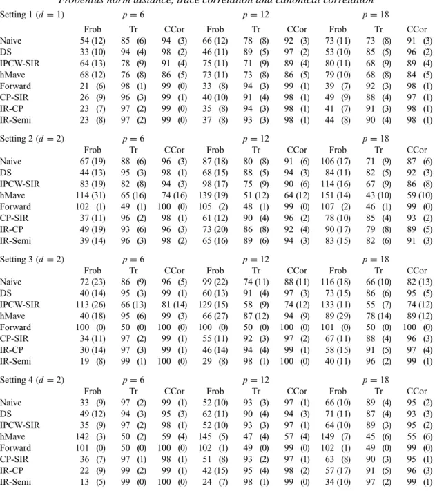
Table 1. Simulation results: mean(×102)and standard deviation(×102, in parentheses)of the Frobenius norm distance, trace correlation and canonical correlation
Setting 1(d=1) p=6 p=12 p=18
Frob Tr CCor Frob Tr CCor Frob Tr CCor Naive 54 (12) 85 (6) 94 (3) 66 (12) 78 (8) 92 (3) 73 (11) 73 (8) 91 (3) DS 33 (10) 94 (4) 98 (2) 46 (11) 89 (5) 97 (2) 53 (10) 85 (5) 96 (2) IPCW-SIR 64 (13) 78 (9) 91 (4) 75 (11) 71 (9) 89 (4) 80 (11) 68 (9) 89 (4) hMave 68 (12) 76 (8) 86 (5) 73 (11) 73 (8) 86 (5) 79 (10) 68 (8) 84 (5) Forward 21 (6) 98 (1) 99 (0) 33 (8) 94 (3) 99 (1) 39 (7) 92 (3) 98 (1) CP-SIR 26 (9) 96 (3) 99 (1) 40 (10) 91 (4) 98 (1) 49 (9) 88 (4) 97 (1) IR-CP 23 (7) 97 (2) 99 (0) 35 (8) 94 (3) 98 (1) 41 (7) 91 (3) 98 (1) IR-Semi 23 (8) 97 (2) 99 (0) 37 (8) 93 (3) 98 (1) 44 (8) 90 (4) 98 (1)
Setting 2(d=2) p=6 p=12 p=18
Frob Tr CCor Frob Tr CCor Frob Tr CCor Naive 67 (19) 88 (6) 96 (3) 87 (18) 80 (8) 91 (6) 106 (17) 71 (9) 87 (6) DS 44 (13) 95 (3) 98 (1) 68 (15) 88 (5) 94 (3) 84 (11) 82 (5) 92 (3) IPCW-SIR 83 (19) 82 (8) 94 (3) 98 (17) 75 (9) 90 (6) 114 (16) 67 (9) 86 (8) hMave 114 (31) 65 (16) 74 (16) 139 (19) 51 (12) 64 (12) 151 (14) 43 (10) 59 (10) Forward 102 (1) 49 (1) 100 (0) 105 (2) 48 (1) 99 (0) 107 (2) 46 (1) 99 (0) CP-SIR 37 (11) 96 (2) 98 (1) 61 (12) 90 (4) 96 (2) 78 (10) 85 (4) 93 (2) IR-CP 49 (19) 93 (6) 96 (3) 73 (20) 86 (8) 92 (4) 90 (17) 79 (8) 89 (5) IR-Semi 39 (14) 96 (3) 98 (2) 65 (16) 89 (6) 94 (3) 83 (15) 82 (6) 91 (3)
Setting 3(d=2) p=6 p=12 p=18
Frob Tr CCor Frob Tr CCor Frob Tr CCor Naive 72 (23) 86 (9) 96 (5) 99 (22) 74 (11) 88 (11) 116 (18) 66 (10) 82 (13) DS 40 (14) 95 (3) 99 (1) 60 (13) 91 (4) 97 (3) 73 (15) 86 (6) 95 (5) IPCW-SIR 113 (26) 66 (13) 81 (14) 129 (15) 58 (9) 74 (12) 133 (11) 55 (7) 74 (12) hMave 40 (18) 95 (6) 99 (3) 66 (27) 87 (12) 94 (9) 89 (29) 78 (14) 89 (12) Forward 100 (0) 50 (0) 100 (0) 100 (0) 50 (0) 100 (0) 101 (0) 50 (0) 100 (0) CP-SIR 34 (11) 97 (2) 99 (1) 55 (11) 92 (3) 97 (2) 67 (11) 88 (4) 96 (3) IR-CP 30 (14) 97 (3) 99 (1) 46 (14) 94 (4) 99 (1) 58 (15) 91 (5) 97 (4) IR-Semi 19 (8) 99 (1) 100 (0) 29 (8) 98 (1) 100 (0) 40 (11) 96 (2) 99 (1)
Setting 4(d=2) p=6 p=12 p=18
Frob Tr CCor Frob Tr CCor Frob Tr CCor Naive 33 (9) 97 (2) 99 (1) 52 (10) 93 (3) 97 (1) 66 (10) 89 (4) 95 (2) DS 49 (12) 94 (3) 95 (3) 62 (11) 90 (4) 94 (3) 71 (11) 87 (4) 93 (3) IPCW-SIR 35 (9) 97 (2) 98 (1) 52 (10) 93 (3) 97 (1) 64 (10) 89 (3) 95 (2) hMave 142 (3) 50 (2) 59 (4) 145 (5) 47 (4) 57 (4) 149 (7) 45 (6) 55 (6) Forward 101 (0) 50 (0) 100 (0) 102 (1) 49 (0) 99 (0) 102 (1) 49 (0) 99 (0) CP-SIR 36 (7) 97 (1) 98 (1) 51 (8) 93 (2) 97 (1) 63 (8) 90 (3) 95 (1) IR-CP 22 (9) 99 (2) 99 (1) 42 (15) 95 (4) 98 (2) 57 (17) 91 (5) 96 (3) IR-Semi 13 (5) 99 (0) 100 (0) 24 (7) 98 (1) 99 (0) 34 (10) 97 (2) 99 (1)
DS, method ofLi et al.(1999); IPCW-SIR, method ofLu & Li(2011); hMave, method ofXia et al.(2010); Forward, forward regression; CP-SIR, the computationally efficient approach; IR-CP, the counting process inverse regres-sion approach; IR-Semi, the semiparametric inverse regresregres-sion approach; Frob, Frobenius norm distance; Tr, trace correlation; CCor, canonical correlation.
double slicing in Settings 3 and 4, respectively. Regarding the three error measurements, the Frobenius norm distance is the most informative, while the trace and canonical correlations are less sensitive to the performances.
Of the two inverse regression methods, the semiparametric version is slightly better in Settings 3 and 4. The main advantage of the semiparametric version compared with the counting process version is its double robustness, which ensures consistency even when the conditional expec-tations are not estimated correctly. However, this theoretical advantage does not translate into strong numerical improvements in Settings 1 and 2, especially whenpis large. This is possibly due to the variations in the hazard function estimation, which introduces numerical instability. In Setting 1, forward regression achieves the best performance. As discussed in Example 1, this method mimics the efficient estimating equations used in the proportional hazards model and is thus the most efficient method in this setting. In Setting 2, the computationally efficient approach performs similarly to the two inverse regression approaches and even outperforms them for largep. This demonstrates the potential of this approach in higher dimensional settings when nonparametric estimation may not be preferred.
One major challenge in solving the estimating equations is the computational burden, especially for equations with nonparametric components. Our method adds difficulties due to the extra orthogonality constraintsBTB=I
d×d. However, by combining the first-order algorithm with the
Rcpp interface, our implementation can solve the estimating equations very efficiently. Also, parallel computing through OpenMP is used to approximate the gradient for each entry of B
numerically. In Setting 2 withp = 6, the mean computational time for the inverse regression counting process approach is only 1.62 seconds, while the time for the semiparametric version is 8.01 seconds. The Supplementary Material summarizes the computational costs. All simulations were done on an Intel Xeon E5-2680v4 processor with five parallel threads.
We further investigate the variance of the proposed methods. Due to the complicated variance formula, we instead use bootstrap to estimate the standard deviations of the proposed estimators. Using an upper block-diagonal version of the parameter of interest, we estimate the standard deviations based on 100 bootstrap samples and also report the 95% confidence intervals. The results show that in Setting 1, the bootstrap estimators of all the proposed methods approximate the standard deviations well. In the other settings, the approximations for the computationally efficient and counting process inverse regression approaches still achieve good performances, while the approximation for the semiparametric inverse regression slightly overestimates the standard deviation, leading to slight overcoverage, around 98%.
5.2. Skin cutaneous melanoma data analysis
We apply the proposed method to The Cancer Genome Atlas (https://cancergenome. nih.gov/) skin cutaneous melanoma dataset, which provides comprehensive profiling data on more than thirty cancer types. We acquired 20 531 items of mRNA expression and clinical data on a total of 469 patients, with 156 observed failures. To produce biologically meaning-ful results, we preselect the top 20 genes highly associated with cutaneous melanoma based on meta-analyses of over 145 papers (Chatzinasiou et al.,2011). A list of these genes can be found at http://bioserver-3.bioacademy.gr/Bioserver/MelGene/. We further include age at diagnosis as a clinical control variable. All covariates are pre-processed to have unit variance and zero mean.
Selecting the number of structural dimensions can be challenging, especially with right-censored survival data (Xia et al.,2010), and we adopt the validated information criterion (Ma &
25
(a) (b)
12
1 0 –1 –2
0.8
0.6 0.4
Survi
v
al
0.2 0 0
1 3
5 10
Survi
val time (years)
15 20
25 20
15
10
5
Survi
v
al time (years)
3
1
0
–3 –2 –1 0 1 2 3
bX
bX
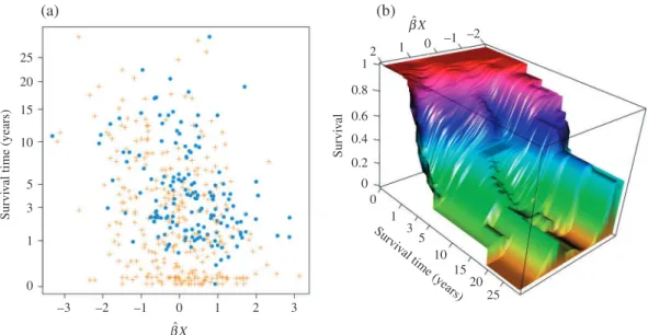
Fig. 1. Fitted direction and survival function of the semiparametric inverse regression: (a) the projected direction versus the observed failure times (blue dots) and censoring times (orange plus signs); (b) a nonparametric estimate of
the survival function based on the projected direction.
validated information criterion is constructed by penalizing the quadratic form of the objective function. When we apply this method to all of our proposed estimating equation approaches,
d =1 always yields the best fit. Hence we present the results for all methods withd =1. As a demonstration of the fitted model, we project the design matrix onto the estimated direction of the semiparametric inverse regression approach and plot the survival outcome against the projection. A nonparametric estimator of the conditional survival function based on this projection is also produced. We can see a clear trend that subjects with larger values of the projection have a lower survival rate. For comparisons, we look at the competing methods with one structural dimension, and the results can be found in the Supplementary Material. It seems that double slicing obtains a similar direction with monotone effects on the risk of failure, while the other directions obtained by other methods are nonmonotone.
Table 2.Skin cutaneous melanoma data analysis results: the loading vectors(×102)of the first structural dimension
Nai
v
e
DS IPCW
-SIR
hMa
v
e
F
orw
ard
CP-SIR IR-CP IR-Semi
Age 16 47 10 0 60 59 53 54
TYRP1 −16 −5 −9 24 18 11 39 30
OCA2 18 17 14 −6 21 19 22 5
TYR −60 −9 −65 −78 −19 −27 −19 9
SLC45A2 11 24 23 14 30 28 16 17
CDKN2A 6 −28 −2 −12 −9 −7 −2 −11
MX2 2 −2 −2 −12 −19 −13 −30 −27
MTAP −15 −8 −10 −14 −31 −36 −35 −30
MITF 56 −9 43 5 −13 −12 2 −27
VDR 5 −18 −9 10 −10 −6 −4 2
CCND1 −20 35 −21 −5 16 17 18 16
MYH7B 10 −27 5 −4 −29 −32 −30 −48
ATM −16 −22 2 28 −4 7 0 6
PLA2G6 −22 −16 −21 7 4 −5 −11 −3
CASP8 15 −39 21 −13 −26 −24 −18 −14
AFG3L1 12 26 18 −15 17 10 −6 −9
CDK10 3 8 2 25 −7 −1 9 8
PARP1 −9 3 −22 17 14 18 8 18
CLPTM1L −8 −5 17 2 −6 −6 −2 −6
ERCC5 −14 25 −17 −7 12 13 22 3
FTO −3 −3 −8 14 15 17 7 5
DS, method ofLi et al.(1999); IPCW-SIR, method ofLu & Li(2011); hMave, method ofXia et al.(2010); Forward, forward regression; CP-SIR, the computationally efficient approach; IR-CP, the counting process inverse regression approach; IR-Semi, the semiparametric inverse regression approach.
effect of the directions. We provide a comparison of the different methods with respect to the Frobenius norm distance in the Supplementary Material.
6. Discussion
efficient approach requires only a singular value decomposition and has satisfactory performance. However, it does not enjoy the same theoretical guarantee without conditions on the covariates. Further relaxation of these conditions is of interest.
Our framework may be extended. First, by imposing penalization on the estimating equations, it is possible to extend the framework to high-dimensional data. Sparse estimation of theBparameter may help interpretations and improves the prediction accuracy of subsequent nonparametric models. Another direction is to search for alternative α functions. In our inverse regression framework, we used the ϕ function, which is motivated by the inverse regression curve of a binary outcome. It would be interesting to investigate the possibility of a sliced average variance estimation-type (Cook & Weisberg,1991) function that may deal with more complicated model structure. We can also consider usingα(u,X)=BTXϕT(u). It would also be interesting to derive
anα function that achieves semiparametric efficiency. Lastly, it would be interesting to extend this framework to a time-varying coefficient setting, where the dimension reduction spaceS(t)
changes over timet.
Supplementary material
Supplementary material available at Biometrika online includes a derivation of the ortho-complement of the nuisance tangent space, proof of the double robustness property for the semiparametric inverse regression approach, proofs of Lemma1and Theorem1, and additional simulation and data analysis results.
Acknowledgement
The first two authors contributed equally to this paper. The authors thank the associate editor and two reviewers for their helpful comments. Q. Sun was partially supported by the Natural Sciences and Engineering Research Council of Canada and a Connaught Award. R. Zhu was partially supported by a Fellowship Award from the National Center for Supercomputing Applications. T. Wang was partially supported by the National Natural Science Foundation of China. D. Zeng was partially supported by the U.S. National Institutes of Health.
References
Behrmann, I.,Wallner, S.,Komyod, W.,Heinrich, P. C., Schuierer, M.,Buettner, R.&Bosserhoff, A.-K.
(2003). Characterization of methylthioadenosin phosphorylase (MTAP) expression in malignant melanoma.Am. J. Pathol.163, 683–90.
Bickel, P. J., Klaassen, C. A., Ritov, Y. & Wellner, J. A. (1993). Efficient and Adaptive Estimation for
Semiparametric Models. Baltimore, Maryland: Johns Hopkins University Press.
Chatzinasiou, F.,Lill, C. M.,Kypreou, K.,Stefanaki, I.,Nicolaou, V.,Spyrou, G.,Evangelou, E.,Roehr, J. T.,
Kodela, E.,Katsambas, A.et al. (2011). Comprehensive field synopsis and systematic meta-analyses of genetic
association studies in cutaneous melanoma.J. Nat. Cancer Inst.103, 1227–35.
Cook, R. D.(2009).Regression Graphics: Ideas for Studying Regressions Through Graphics. New York: John Wiley
& Sons.
Cook, R. D.&Weisberg, S.(1991). Discussion of sliced inverse regression for dimension reduction.J. Am. Statist.
Assoc.86, 328–32.
Cox, D. R.(1972). Regression models and life-tables.J. R. Statist. Soc.B34, 187–220.
Dong, Y.&Li, B.(2010). Dimension reduction for non-elliptically distributed predictors: Second-order methods.
Biometrika97, 279–94.
Edelman, A.,Arias, T. A.&Smith, S. T.(1998). The geometry of algorithms with orthogonality constraints.SIAM
J. Matrix Anal. Appl.20, 303–53.
Gudbjartsson, D. F.,Sulem, P.,Stacey, S. N.,Goldstein, A. M.,Rafnar, T.,Sigurgeirsson, B.,Benediktsdottir,
K. R.,Thorisdottir, K.,Ragnarsson, R.,Sveinsdottir, S. G.et al. (2008). ASIP and TYR pigmentation variants
Hansen, L. P. (1982). Large sample properties of generalized method of moments estimators.Econometrica50, 1029–54.
Li, B.&Dong, Y.(2009). Dimension reduction for nonelliptically distributed predictors.Ann. Statist.37, 1272–98.
Li, B.&Wang, S.(2007). On directional regression for dimension reduction.J. Am. Statist. Assoc.102, 997–1008.
Li, C.,Zhao, H.,Hu, Z.,Liu, Z.,Wang, L.-E.,Gershenwald, J. E.,Prieto, V. G.,Lee, J. E.,Duvic, M.,Grimm, E. A.
et al. (2008). Genetic variants and haplotypes of the caspase-8 and caspase-10 genes contribute to susceptibility to cutaneous melanoma.Hum. Mutat.29, 1443–51.
Li, K.-C.(1991). Sliced inverse regression for dimension reduction.J. Am. Statist. Assoc.86, 316–27.
Li, K.-C.,Wang, J.-L.&Chen, C.-H.(1999). Dimension reduction for censored regression data.Ann. Statist.27,
1–23.
Lin, D.,Wei, L.&Ying, Z.(1998). Accelerated failure time models for counting processes.Biometrika85, 605–18.
Lu, W.&Li, L.(2011). Sufficient dimension reduction for censored regressions.Biometrics67, 513–23.
Ma, Y.&Zhang, X.(2015). A validated information criterion to determine the structural dimension in dimension
reduction models.Biometrika102, 409–20.
Ma, Y.&Zhu, L.(2012). A semiparametric approach to dimension reduction.J. Am. Statist. Assoc.107, 168–79.
Nocedal, J.&Wright, S. J.(2006).Numerical Optimization. New York: Springer.
R Development Core Team(2019).R: A Language and Environment for Statistical Computing. Vienna, Austria: R
Foundation for Statistical Computing. ISBN 3-900051-07-0, http://www.R-project.org.
Silverman, B. W.(1986).Density Estimation for Statistics and Data Analysis. Boca Raton, Florida: CRC Press.
Tsiatis, A.(2007).Semiparametric Theory and Missing Data. New York: Springer.
Weisberg, S.(2002). Dimension reduction regression in R.J. Statist. Software7, 1–22.
Wen, Z.&Yin, W.(2013). A feasible method for optimization with orthogonality constraints.Math. Program.142,
397–434.
Wu, T.,Sun, W.,Yuan, S.,Chen, C.-H.&Li, K.-C.(2008). A method for analyzing censored survival phenotype
with gene expression data.BMC Bioinformatics9, 417.
Xia, Y.(2007). A constructive approach to the estimation of dimension reduction directions.Ann. Statist.35, 2654–90.
Xia, Y.,Zhang, D.&Xu, J.(2010). Dimension reduction and semiparametric estimation of survival models.J. Am.
Statist. Assoc.105, 278–90.
Zeng, D.&Lin, D.(2007). Maximum likelihood estimation in semiparametric regression models with censored data
(with Discussion).J. R. Statist. Soc.B69, 507–64.
Zhao, R.,Zhang, J.&Zhu, R.(2017).orthoDr: An Orthogonality Constrained Optimization Approach for
Semi-Parametric Dimension Reduction Problems. R package version 0.3.0.
Zhu, L.,Miao, B.&Peng, H.(2006). On sliced inverse regression with high-dimensional covariates.J. Am. Statist.
Assoc.101, 630–43.