Alex Liberzon1,∗, Roi Gurka1,∗∗, Iztok Tiselj2, Gad Hetsroni1
1Faculty of Mechanical Engineering, Technion – IIT, Haifa 32000, Israel 2Reactor Engineering Division, Jozef Stefan Institute, Ljubljana, Slovenia Received October 22, 2003 / Accepted September 29, 2004
Published online February 8, 2005 –Springer-Verlag 2005 Communicated by T.B. Gatski
Abstract. The topology of large scale structures in a turbulent boundary layer is
investi-gated numerically. Spatial characteristics of the large scale structure are presented through an original method, proper orthogonal decomposition (POD) of the three-dimensional vorticity fields. The DNS results, obtained by Tiselj et al. [23] for a fully developed turbulent flow in a flume, are used in the present work to analyze coherent structures with the proposed method-ology. In contrast to the reconstruction methods that use instantaneous flow quantities, this approach utilizes the whole dataset of the numerical simulation. The analysis uses one thou-sand 3D vorticity fields from 50 000 time steps of the simulation for the Reynolds number of 2600 (the turbulent Reynolds number Re∗=171). The computational domain is 2146×171× 537 wall units and the grid resolution is 128×65×72 points (in streamwise, wall-normal and spanwise directions, respectively). Experimental results obtained by using particle image ve-locimetry (PIV) in a fully developed turbulent boundary layer in a flume, which were analyzed with the same statistical characterization method, are in agreement with the DNS analysis: the dominant vortical structure appears to have a longitudinal streamwise orientation, an inclina-tion angle of about 8◦, streamwise length of several hundred wall units, and a distance between the neighboring structures of about 100 wall units in the spanwise direction.
Key words: direct numerical simulation, vorticity, proper orthogonal decomposition, coherent
structure
PACS: 47.27.Nz, 47.54+r
List of symbols
a Coefficients of the POD eigenfunctions
h Water height, [m]
x,x1,x2,x3 Vector, streamwise, wall normal and spanwise coordinates, [m]
Correspondence to: G. Hetsroni (e-mail: [email protected])
u1,u2,u3 Streamwise, wall normal and spanwise velocity components, [m/s] C Covariance matrix
K Number of POD eigenfunctions, used for reconstruction
L Length, [m]
N Number of vorticity fields
M Number of snapshots
R Two-point correlation tensor ε Reconstruction error φ(i) The ith eigenfunction
ϕ Eigenfunction of the covariance matrix λ(i) The ith eigenvalue
ω,ωˆ Fluctuating and reconstructed vorticity vector fields, [1/s]
Superscripts and subscripts
f+ Quantity in non-dimensional wall units
fk kth vector of the ensemble f∗ Complex conjugate
fi, fj The ith, jth component of the vector field, i,j=1,2,3
1 Introduction
Many turbulent flows display some combination of coherent structures and seemingly disorganized tur-bulent velocity fluctuations (Robinson [17]). In the wall region of the turtur-bulent boundary layer, coherent structures account for over 80% of the energy in the turbulent fluctuations. The coherent structures burst, transferring energy from large to small scales and producing turbulent fluctuations (Robinson [17]). How-ever, their connection to the vorticity, rate of strain, Reynolds stresses and their role in the energy production and dissipation mechanisms, remains unclear (Tsinober [24]). Moreover, their three-dimensionality and time dependence prevents reaching a consensus regarding the shape and spatial characteristics of the coherent structures in the turbulent boundary layer. Hairpin vortices (Smith and Walker [21]), hairpin packets (Adrian et al. [1]), horseshoe vortices (Theodorsen [22]), funnel vortices (Kaftori et al. [8]), and near-wall longitudi-nal vortices (Schoppa and Hussain [18]), are only part of the conceptual models resulting from the extensive experimental and numerical research. One of the exceptions is the low- and high-speed streaks that are prob-ably the most dominant and approved coherent features of the turbulent boundary layer flow (Kline et al. [9]). Despite the variety of models, the experimental (Kaftori et al. [8], Head and Bandyopadhyay [5], Adrian et al. [1]) and numerical (Moin and Moser [13], Zhou et al. [25]) results show that various models have simi-lar spatial characteristics: an inclination angle of approximately 8–12◦, and prominent streamwise extension of the large streamwise-oriented vortical structure.
The investigation of the mechanisms that produce and control the coherent structures, requires the iden-tification of the coherent patterns in a multi-dimensional database. Numerous ideniden-tification techniques have been proposed and implemented on the results of numerical simulations and experiments, for example, by Bonnet et al. [3]. However, there is a need for a statistical description of the three-dimensional information, extracted from the numerical and experimental data.
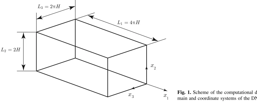
Fig. 1. Scheme of the computational
do-main and coordinate systems of the DNS
and close to the wall, oriented in streamwise direction, with characteristic spatial parameters, such as non-dimensional length x+1 ≈1000, and an expansion angle≈8◦. Most often, these vortices appear as unequal pairs, separated by approximately 100 wall units.
This work presents a characterization method of the flow near the wall that resolves the most energetic coherent structures from a direct numerical simulation (DNS) dataset, provided over a denser grid, than that of the PIV measurements. The DNS solution of the time dependent, three-dimensional Navier–Stokes equa-tions is obtained by Tiselj et al. [23] for a fully developed turbulent flow in a flume, at Reynolds number of 2600. The calculations are carried out in a computational domain of L+1 ×L+2 ×L+3 =2146×171×537 wall units in the x1,x2, and x3directions, respectively. The dominant vortical structures are characterized by using the POD-based analysis of the three-dimensional fields of the vorticity fluctuations. The results are shown as cross sections of the reconstructed vorticity fields in the streamwiseω1ˆ , wall-normalω2ˆ , and spanwiseω3ˆ directions, respectively.
The following Sect. 2 presents the details of the direct numerical simulation method. The characterization method, based on the POD analysis of vorticity, is described in Sect. 3, the methodology is defined in Sect. 4, and is followed by the results and discussion in Sect. 5. Section 6 contains the summary and concluding remarks.
2 DNS
The DNS results, obtained by Tiselj et al. [23] for a fully developed turbulent flow in a flume, are used in the present study to characterize the coherent structures. Details of the numerical method and the conven-tional analysis of the results are described in Tiselj et al. [23] and in the following section only the main characteristics are presented.
The DNS solved the time dependent, three-dimensional Navier–Stokes equations, along with the conti-nuity equation in a rectangular domain. The flow geometry is shown in Fig. 1. The flow driving force was a constant streamwise pressure gradient, while the boundary conditions were: a no slip condition on the bottom wall and a free slip on the free surface. In addition, in the streamwise and spanwise directions, peri-odic boundary conditions were imposed. The pseudo-spectral numerical method was implemented to solve the equations, along with the Fourier expansions of all quantities in the approximately homogeneous direc-tions, x1,x3. The wall normal direction, x2 was presented by Chebyshev polynomials (Tiselj et al. [23]). The present results use the simulation data for the Reynolds number of 2600, or alternatively, the turbu-lent Reynolds number Re∗=171. The calculations were carried out in a computational domain of L+1 ×
step∆t+was 0.05124 in wall units. Instantaneous fields, for the consequential POD analysis, were saved every 2.56 time wall units (every 50 simulation time steps). These parameters define the computational ef-fort of about 40 CPU hours on a SUN Fire 900 MHz processor and 200 MB of RAM. A further limitation is the POD analysis, as it is defined in Sect. 3, that requires 2GB of RAM for the chunk of 250 instantaneous fields. The POD analysis of the full dataset of 1000 instantaneous vorticity fields would require the memory size of about 7 GB. The POD analysis for the short data series of 50 fields was performed on a PC running Matlab and the self-developed code with 512 MB RAM. The analysis of 250 fields chunks was computed with Fortran on SUN Fire 900 MHz, 2 GB RAM, with the modified principal component analysis subroutine (pca.f), which is a part of the multivariate data analysis package in S-Plus/R [14].
3 Proper orthogonal decomposition (POD)
In this section, the background of the POD is described briefly and some details regarding the POD of the vorticity vector fields are presented.
In a most general sense, the proper orthogonal decomposition is equivalent to the Karhunen-Lo´eve decomposition procedure, and it was introduced by Lumley [12] in the context of the turbulence and coherent structures. The procedure, applied to any random, non-homogeneous field f(x)finds the most optimally cor-related feature from the given ensemble of field realizationsfk,k=1. . .N. The decomposed empirical
eigenfunctions are usually referred to as coherent structures, since they are highly correlated in an average sense with the flow field (Berkooz et al. [2], Holmes et al. [6]).
The most probable or “most similar” (Berkooz et al. [2]) structure is proved to be an eigenfunction from the set{φn}, n=1. . .N of the two-point correlation tensor R(x,x)= f(x)f∗(x):
R(x,x)φ(x)dx=λφ(x). (1)
The whole set of the eigenfunctions or proper orthogonal modes allows one to reconstruct any mem-ber of the ensemble fk, by using random uncorrelated coefficients akn that are the square roots of the eigenvaluesλn:
fk(x)= N
n=1
ankφn(x). (2)
It is possible, however, to build a low-order model of the random field by reconstruction on the base of only K first eigenmodes (assuming a descending order of the eigenvaluesλn> λn+1):
ˆ
fk(x)= K
n=1
ankφn(x). (3)
The quality of the low-order model could be characterized by the error introduced by truncating the full series of the eigenmodes to the desired order. For example, we define the error of the approximation as the relative error:
ε=
N
k=1
fk(x)− ˆfk(x)2
|fk(x)|2 . (4)
3.1 Construction of snapshots and POD basis functions
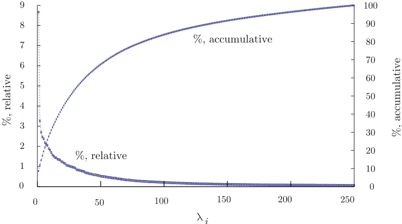
Fig. 2. Relative and cumulative percentage of the enstrophy of the eigenvalues
Nx1×Nx2×Nx3grid points and expressed as a vector (where →
ω= [ω1, ω2, ω3]T) of the length n=3·N x1·
Nx2·Nx3 as follows:
→
ωk=
→
ωk1 ...
→
ωkn
(5)
Instead of the two-point correlation tensor we construct the symmetric matrix from the ensemble set
ωk,k=1. . .N as follows:
C=→ω−→ωT→ω−→ω, (6)
where superscriptT denotes the transpose operator. The efficiency of the “snapshots” method (Sirovich [19]) is obvious when the number of snapshots M is significantly less than the number of the three-dimensional grid points. The eigensolutions,ϕof this matrix satisfy the following equation:
Cϕ=λϕ , (7)
from which the POD modes are calculated through the projection on the original fields:
φ(n)= M
j=1 ϕ(n)
j →
ωj, (8)
whereϕ(jn)is the jth element of the eigenvectorϕ, corresponding to the nth eigenvalueλ(n).
It is noteworthy that the above relationships are valid both for scalar functions such as the vorticity com-ponentsωi,i=1,2,3 (which we have used in our experimental analysis, Liberzon et al. [11]), and for the
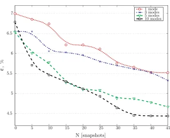
Fig. 3. Relative error (Eq. (4)) between the instantaneous vorticity fields and the low-order reconstruction
3.2 POD dimension
The problem to define the dimension K through the POD modes, which is also known as the problem of low-order representation, has been addressed many times (e.g., Berkooz et al. [2], Holmes et al. [6], Sirovich [20]). The most widely used definition, proposed by Sirovich [20], suggests that the amount of the captured energy defines the number of modes. However, Berkooz et al. [2] pointed out that a relatively large number of eigenfunctions is required to capture a significant amount of the kinetic energy, when the full flow domain is taken as the domain for computation of the eigenvalues. Indeed, Fig. 2 depicts the amount of relative energy of the eigenmodes, relative to the energy in the full flow domain.
In the present study we propose to follow the idea of the “compactness in space” (Moin and Moser [13]), and their term “characteristic eddy”, originally introduced by Lumley [12]. The minimal number of modes is not defined by an arbitrary threshold of the captured energy. Instead, it is defined by the number of modes that delimits the compact (in space) structure, which does not change its shape with combination of addi-tional modes, and the truncation error ε(Eq. 4) is reasonably small. The truncation error analysis of the presented reconstruction, as a function of the number of snapshots, is shown in Fig. 3. It is clear that even for relatively low number of snapshots, the reconstructed vorticity fields truly reproduce the original snapshots, with the error of≈5%.
4 Methodology
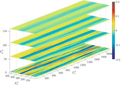
Fig. 4. POD analysis of the wall normal vorticity component,ω2of the DNS data
Velocity and vorticity are two major flow quantities that can be used for identification of coherent struc-tures, as they contain all the necessary information about the turbulent flow. The velocity field in the turbulent boundary layer is apparently affected more by the average streamwise velocity fluctuations (i.e., jitter ef-fect). Moreover, it was shown that vorticity is a more appropriate choice for the spatial characterization of the coherent structures (especially when the decomposition operator is involved) in the back-step (Kostas et al. [10]) and in a turbulent boundary layer flows (Liberzon et al. [11]).
Contrary to the identification of the pre-defined model, we suggest that the characterization approach has to fulfill the three basic guidelines: (1) data analysis is performed without threshold operation, and the same filters are applied to all data; (2) data is statistically significant, thus characterizes the structure that exists over a period of time, and (3) the analysis is based on a flow characteristic that strongly represents turbulence (e.g., vorticity), in order to be objective and free of any user-selected threshold.
In this study, the reconstruction method, similar to that proposed by Gordeyev and Thomas [4], is de-veloped, aiming at a description of the “large scale structure”:
ˆ ω(x)=
K
n=1
λ(n)φ(n)(x) K N (9)
The reconstruction operator follows the concept of the “characteristic eddy” investigated by Lumley [12] and it fulfills the above-defined guidelines.
5 Results and discussion
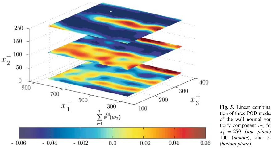
Fig. 5. Linear
combina-tion of three POD modes of the wall normal vor-ticity componentω2 for
x+2 =250 (top plane), 100 (middle), and 30 (bottom plane)
and spanwise directions, respectively. This analysis allows a visual comparison between the numerical and the two-dimensional experimental results.
In order to gain a better understanding of the association of our results with known coherent structures, the cross sections of the wall normal component of the POD reconstructionω2ˆ are presented in Fig. 4. The features that are depicted in Fig. 4 resemble the low-speed streaks phenomena. The low-speed streaks are characterized in the streamwise-spanwise plane as alternating zones in the spanwise direction of positive and negative velocity fluctuations. Obviously, the velocity gradients have similar spatial characteristic view. In Fig. 4, the colors present the intensity of the vorticity, by magnitude and sign. Counter-changing patches of the positive (red, grayscale in the print version) and negative (blue) fluctuating vorticity emphasize the regions of the low and high-speed streaks. A more detailed inspection of the POD modes in these planes pro-poses that the characteristic spanwise separation (i.e., the distance between two neighbor pair of alternating patches), close to the wall, is of the order of one hundred wall units, which is known as a streak spacing, λ+≈100 (Kline et al. [9]). Moreover, the streamwise dimension of these color patterns is approximately
several hundred wall units (i.e., x1+≈600−1000), which is in good agreement to the length of the streaks (Panton [16]). We observe that vorticity is relatively strong in the buffer region (x2+≈30), it almost vanishes closer to the wall, and also significantly reduces at larger x2+distances.
Similar results were obtained in our experimental study (Liberzon et al. [11]), in which coherent struc-tures in turbulent boundary layer in a flume were characterized by using particle image velocimetry. The POD analysis was performed exactly within the same framework, but on the scalar fields of the vorticity components, differentiated from the measured two-dimensional and two-component velocity fields. The ex-periments were conducted in a horizontal flume of 4.9×0.32×0.1 meter, at Reh=24 000, based on the
water height, h. The measurement planes were located at x2+=50,150,250 and 400 images were taken at each location in order to measure streamwise–spanwise velocity fields and the wall normal component of the vorticity,w2. The linear combination of three first POD modes of the scalar fields ofw2is shown in Fig. 5. The topological features obtained from the DNS data are in good agreement with the experimental results.
Figure 6 presents the cross-sectional planes of the POD analysis of the streamwise vorticity component ω1. Here, the inside view of the coherent structure is demonstrated by means of the vorticity projections onto the cross sectional planes. In a similar manner, Fig. 7 depicts the three- dimensional projection of the spanwise vorticity component.
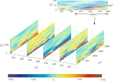
Fig. 6. POD analysis of the streamwise vorticity component, combination of the first three POD modes ofω1
Fig. 7. POD analysis of the spanwise vorticity component, combination of the first three modes ofω3
[image:9.595.87.464.366.647.2]Comparing with the previous results: the inclination angle of the pattern and the streamwise length of approximately 800 wall units are in good agreement with the results obtained by Jeong et al. [7], in which the identification of the coherent structures from DNS of a three-dimensional channel flow was performed by using the intermediate eigenvalue of the gradient tensor invariant. In addition, this pattern is in consen-sus with the double-structure model proposed by Nezu and Nakagawa [15] for turbulent boundary layers in open-channel flows: small-scale (e.g., bursting) motions and the large-scale vortical motions. In this double-structure conceptual model, the initially small-scale hairpin vortices agglomerate and form a large-scale motion, very similar to the shape demonstrated in this study. Adrian et al. [1] reported, based on their ex-perimental results, that the most probable “hairpin packet” growth angle is 10.5◦, and the streamwise length of this large scale structure (i.e., hairpin packet) is of the order of 1.3–2δ, whereδis the thickness of the boundary layer (δ≈1000 wall units).
The geometrical characteristics of the presented pattern are in good agreement with the listed references, and it is also consistently shown by the streamwise length of the large pattern in the field of the spanwise vorticityω3in Fig. 7. This plot provides the clearest perspective of the organized turbulent structure in the turbulent boundary layer in x1–x2plane. The footprints of the strong vortical motions, represented by pairs of the opposite-sign vorticity regions (inclined and elongated in the streamwise direction), are shown in par-allel spanwise cross sections of the flow field. Emphasis is given to a large scale structure that emerges from the wall toward the mean flow. The structure is symmetrical around an inclined axis, which is shown by suc-cessive red and blue contours, and the length and the angle of the contours characterize the topology of the projection on x1–x2plane. It is noteworthy, that the distance between the spanwise cross sectional planes in Fig. 7 is chosen arbitrarily.
The main drawback of the proposed method is that it is not suitable for the extraction of the small struc-tures, such as hairpins (Smith and Walker [21], Zhou et al. [25]), the arch of a horseshoe (Robinson [17]) or elongated quasi-streamwise vortices (Schoppa and Hussain [18]), observed in the turbulent boundary layer. From the detailed inspection of the present results we can conclude that the identified structure apparently has all the parameters of a large-scale, funnel vortices, proposed by Kaftori et al. [8].
6 Summary and conclusions
A numerical study of coherent structures embedded in a turbulent boundary layer was performed aiming at achieving better understanding of the transfer phenomena. In addition to the previously published ex-perimental dataset, the numerical simulation dataset presented in this work, served the novel identification technique of coherent structures in boundary layer flow. This communication presents the identification of the underlying coherent structure by employing linear combination of the POD modes of the three-dimensional vorticity vector fields.
Summing up the results of the two-dimensional projection characterizations and the reconstruction of the three-dimensional model by means of iso-surfaces, we provide the following list of the spatial characteristics of the identified quasi-streamwise vortical structures:
– The length of the structures is approximately 1000 wall units;
– The structures are inclined in the x1–x2plane in an angle of 8◦–10◦upward from the bottom;
– The spanwise separation of the structures is≈100 wall units;
The three-dimensional representation leads to a picture of the large scale, quasi-streamwise vortical struc-ture, elongated in the streamwise direction that has the shape similar to a “funnel” (Kaftori et al. [8]). The structure has its origin in the near wall region (x2+≤20) and develops toward the outer region of the bound-ary layer.
7. Jeong, J., Hussain, F., Schoppa, W., Kim, J.: Coherent structures near the wall in a turbulent channel flow. J. Fluid Mech.
332, 185–214 (1997)
8. Kaftori, D., Hetsroni, G., Banerjee, S.: Funnel-shaped vortical structure in wall turbulence. Phys. Fluids 6, 3035–3050 (1994)
9. Kline, S.J., Reynolds, W.C., Schraub, F.A., Runstadler, P.W.: The structure of turbulent boundary layers. J. Fluid Mech. 30, 741–773 (1967)
10. Kostas, J., Soria, J., Chong, M.S.: PIV measurements of a backward facing step flow. In: Proc. 4th Int. Symposium on
Particle Image Velocimetry, Gottingen, Germany (2001)
11. Liberzon, A., Gurka, R., Hetsroni, G.: Vorticity characterization in a turbulent boundary layer using PIV and POD analysis. In: Proc. 4th Int. Symposium on Particle Image Velocimetry, p. 1184, Gottingen, Germany (2001)
12. Lumley, J.L.: Stochastic Tools in Turbulence, Applied Mathematics and Mechanics, vol. 12. Academic, New York (1970) 13. Moin, P., Moser, R.: Characteristic-eddy decomposition of turbulence in a channel. J. Fluid Mech. 200, 471 (1989) 14. Murtagh, F.: Multivariate data analysis software in S-plus/R, http://astro.u-strasbg.fr/ fmurtagh/mda-sw/splus/ (2002) 15. Nezu, I., Nakagawa, H.: Turbulence in open-channel flows. IAHR Monograph Series, A.A. Balkema, Rotterdam (1993) 16. Panton, R.L.: Self-Sustaining Mechanisms of Wall Turbulence, Advances in Fluid Mechanics, vol. 15. Computational
Me-chanics Publications, Southampton, UK (1997)
17. Robinson, S.: Coherent motions in the turbulent boundary layer. Annu. Rev. Fluid Mech. 23, 601–639 (1991) 18. Schoppa, W., Hussain, F.: Coherent structure dynamics in near-wall turbulence. Fluid Dyn. Res. 26, 119–139 (2000) 19. Sirovich, L.: Turbulence and the dynamics of coherent structures, part I: coherent structures. Q. Appl. Math. XLV, 561–571
(1987)
20. Sirovich, L.: Chaotic dynamics of coherent structures. Physica D, 37, 126 (1989)
21. Smith, C.R., Walker, J.D.A.: Turbulent wall-layer vortices. In: Green S. (ed.) Fluid Vortices, pp. 235–283. Kluwer, Amster-dam (1995)
22. Theodorsen, T.: Mechanism of turbulence. In: Proc. 2nd Midwestern Conference on Fluid Mechanics (1952)
23. Tiselj, I., Pogrebnyak, E., Li, C., Mosyak, A., Hetsroni, G.: Effect of wall boundary condition on scalar transfer in a fully developed turbulent flume. Phys. Fluids 13, 1028–1039 (2001)
24. Tsinober, A.: Vortex stretching versus production of strain/dissipation. In: Hunt J., Vassilicos J. (eds.) Turbulence Structure
and Vortex Dynamics, pp. 164–191. Cambridge University Press, Cambridge (2000)