A noncooperative marriage model with remarriage
Michael Malcolm
Received: 7 November 2009 / Accepted: 12 November 2010 / Published online: 8 December 2010
Springer Science+Business Media, LLC 2010
Abstract I propose a noncooperative marriage model that explicitly accommodates the possibility of endogenous exit and remarriage, and where marriages are of variable quality. The fundamental innovation is that the remarriage decision is infinitely repeated and the problem is fully stationary, reflecting the contemporary reality in marriage markets. I show that cooperative behavior within marriage is possible in subgame perfect equilibrium both in a setting where marriage quality is independently drawn and in a setting with persistent spouse-specific characteristics and an evolving marriage market quality. I show that spouses engage in cooperative behavior most easily when they have intermediate patience levels, which is a non-standard but intuitive game theoretic result in this setting. This model also contributes to the game theory literature by proposing another avenue for sustained cooperation in a repeated prisoner’s dilemma with endogenous exit: randomness in payoff streams.
Keywords Divorce Remarriage Repeated prisoner’s dilemma Game theory
Household economics
JEL Classification D13C73J12
1 Introduction
Models of family interactions rest on the assumption that there is some reward to be gained from cooperative family interactions. With respect to marriage,1
M. Malcolm (&)
Department of Economics, American University of Sharjah, PO Box 26666, Sharjah, United Arab Emirates
e-mail: [email protected]
1
Becker (1973) observed that ‘‘since marriage is practically always voluntary… per-sons marrying can be assumed to raise their utility level above what it would be were they to remain single.’’ However, incentives within marriage may not be aligned, allowing one spouse to increase his or her payoff at the other spouse’s expense. Furthermore, married spouses face a range of outside options other than perpetual cooperative behavior with their current spouses, and recent work is increasingly recognizing that the most relevant outside option is remarriage.
Marriage markets today exhibit high and growing turnover. Chiappori and Weiss (2006) note that remarriage rates for young people have risen so far that they are equalto initial marriage rates. Consistent with these stylized facts, this paper is the first to propose an endogenous and fully stationary model of the marriage and remarriage market with infinite repetition. That is, upon divorce, spouses face a reiteration of the same problem that they initially faced (with possible evolution in the average quality of available partners).
I model behavior within marriage using a public goods framework with the structure of a prisoner’s dilemma, similar to Lundberg and Pollak (1994) and Andaluz and Molina (2007). However, the cooperative payoff is random and partner-specific; some matches induce a higher cooperative payoff than others. In addition to choosing their within-marriage strategies, matched spouses also decide each period whether to stay married or to divorce and reenter the marriage market. I show that there are cooperative equilibria even allowing for this endogenous exit. I consider both a stationary model, where each match quality is drawn from the same distribution, and a dynamic model with persistent player-specific character-istics, allowing for the possibility of evolution in the quality of unmatched spouses. A surprising result is that ease of cooperation is nonmonotonic in players’ discount factors. Extremely impatient spouses are unlikely to enter into cooperative marriages because they overvalue short-term deviations from a cooperative equilibrium. At the same time, extremely patient spouses are also unlikely to enter into cooperative marriages since they face little discounting by waiting for a higher-quality match.
In addition to this paper’s context in the marriage literature, the model is nested within a subset of the repeated games literature on games with endogenous exit. This paper does seem to be the first use of a model from this class in the context of a marriage market.
Section2reviews the relevant literature. Section3presents the stationary model. Section4presents the dynamic model and comparative statics. Section5concludes and discusses extensions.
2 Related literature
options.2This model in this paper is game-theoretic, and the relevant outside option is remarriage.
Lundberg and Pollak (1994) further classify game theoretic models into cooperative and noncooperative variants, though the line between the two is becoming increasingly blurred. Cooperative models rely upon an assumption that spouses can enter into agreements that are binding and costlessly enforceable. In contrast, noncooperative models require that cooperation be self-enforcing. While cooperative models largely dominate the literature, many authors continue to argue forcefully that noncooperative elements are important. Lundberg and Pollak (2007) assert that changing norms and institutions render enforceable agreements increasingly infeasible. This constrains available options within marriage and creates inefficiencies, potentially including divorce (Lundberg and Pollak2003).3 Stevenson (2007) finds that investment in many types of marriage-specific capital fell as a result of the increasing ease of divorce.
I model behavior within marriage using the infinitely-repeated public goods-provision framework adopted by Lundberg and Pollak (1994) and by Andaluz and Molina (2007).4The cooperative strategy is optimal provision of a within-marriage public good, but each player can defect to generate a higher payoff at his or her partner’s expense.5The treatment of allocationwithinmarriage is relatively simple in order to shed light on the remarriage issue. At the end of each period, either spouse can divorce and restart the same interaction with a new partner.
Chiappori et al. (2009a, b) introduce a model that incorporates divorce and remarriage. The model is a hybrid of cooperative and noncooperative elements in the sense that allocation within marriage is governed by a bargaining process, but players can unilaterally exit. Their model shares key features with this model, namely matching and a match-specific quality that affects payoffs. However, the model is only two periods, and they solve fully only for the case in which all players marry in the first period. They explore the more general case but point out that the problem is difficult to solve because of strategic postponement of marriage and declining quality of the marriage pool. The model in this paper incorporates both of these issues fully.
Chiappori and Weiss (2006) also utilize a model with remarriage to demonstrate that a higher divorce rate might actually be welfare-improving by making remarriage easier. The critical difference is that the remarriage rate is exogenously set in their model.
Repeated prisoner’s dilemmas with endogenous exit are not new to game theory. The earliest example seems to be due to Schluessler (1989). I cannot find an example of their application to this setting, although in ‘‘Leaving the Prison:
2
Possibilities are terminal divorce (Manser and Brown 1980), suboptimal behavior withinmarriage (Lundberg and Pollak1994) or even suicide (Hoddinott and Adam1998).
3
Divorce is terminal in this model.
4 The former note that, by an application of the folk theorem, any payoff that is feasible and individually
rational is a possible subgame perfect equilibrium payoff of the repeated game.
5 The nature of the strategies chosen within marriage varies widely within the literature. Examples are
Permitting Partner Choice and Refusal in Prisoner’s Dilemma Games’’, Hauk (2001) suggests that such a model may be applicable to dating.
Usualstationarystrategies (i.e. the strategy can be restarted with any player at any time) that support mutual cooperation in every period, like tit-for-tat or grim trigger strategies, are no longer equilibria.6A small literature has developed that proposes ways to sustain cooperation in such a setting, many of which are informative in a marriage context. The idea is to impose some kind of cost associated with exiting and finding a new partner.
Mailath and Samuelson (2006) propose a fixed number of periods of defection with each new partner before cooperation can begin. Indeed, most relationships involve a probationary period before commitment begins and one can interpret steadily rising pre-marriage cohabitation, as documented by Stevenson and Wolfers (2007), in this context. Also, the first match may be fundamentally different than subsequent matches if social custom attaches a stigma to divorce. Carmichael and Macleod (1997) suggest an exogenous cost associated with quitting and finding a new partner. Courtship costs and wedding rings are entry costs, while child-support payments are exit costs. Datta (1996) allows the payoff each period to grow geometrically with the number of periods one has been in a relationshipwith the current partner. If there is relationship-specific capital accumulated in marriage, then this is germane to our example. Ghosh and Ray (1996) propose an environment where there are some proportion of ‘‘bad’’ players who always defect, and so separating and finding a new partner introduces a risk of encountering a serial defector. In this paper, partner-specific payoffs form a new avenue for cooperation.
3 A stationary model
We begin by describing the interaction within a marriage, followed by a discussion of the matching and remarriage process. Assuming that players remain married, the following problem is repeated each period. Each partneri=1, 2 allocates resources to a private goodwor to a marriage-specific public goodg. This can be interpreted broadly to incorporate allocation not just of financial resources, but also of time, goodwill, etc. Utility is quasilinear in the public good:
U1¼w1þf gð 1;g2Þ U2¼w2þf gð 1;g2Þ ð1Þ
The public good payoff functionf() is assumed to be strictly increasing and strictly concave in both arguments. Normalizing the cost of the private good to 1, each agent is subject to a resource constraint:
wiþPggi¼Yi ð2Þ
Formulating this interaction as a game, the two relevant strategies are a cooperative strategy (C) where the spouses coordinate to provide the efficient level of the public
6
good and a noncooperative strategy (D) where each spouse unilaterally maximizes utility. An asymmetric outcome, with one spouse defecting against the other’s cooperative behavior, is also possible. The payoffs for mutual cooperation within marriage are weighted byx, which is a randomU(0, 1) match-specific quality. The strategic form of the game is shown below.Uimndesignates playeri’s payoff when
player 1 chooses strategymand player 2 chooses strategyn(Table 1).
Given the structure of the spousal optimization problem in (1) and (2), the following inequalities characterize the payoff structure:
U1CCþU2CC[UDD1 þU2DD ð3Þ
UDC1 [UCC1 ;UCD2 [U2CC ð4Þ
U1CD\UDD1 ;U2DC\U2DD ð5Þ
Proofs of these inequalities are given in ‘‘Appendix 1’’, but the logic is clear. The problem has the structure of a prisoner’s dilemma, where (3) shows that some surplus results from mutual cooperation relative to unilateral utility-maximization. The inequalities in (4) show that defecting against a cooperator is more profitable for the defector than mutual cooperation, at least in a single repetition of the stage game; the inequalities in (5) show that this isworsefor the cooperator even than mutual defection.
We parameterize the within-marriage interaction by normalizing the mutual defection payoff to 0. Letting the surplus from the cooperation equal 4, we allow for an unequal distribution of the marital surplus, so that the agents’ payoffs are 2?aand 2-a, wherea\1 reflects the degree of asymmetry in the division of marital surplus.7 The mutually cooperative outcome is weighted by the match-specificx, discussed below. Consistent with the inequalities in (4) and (5), we will let defection against a cooperator generate a payoff of 3, while being defected against while cooperating generates a payoff of-1. Again, the important point is that the problem has the structure of a prisoner’s dilemma (Table2).
The timing of the game is as follows. There is a continuum of potential spouses. At the beginning of each period, all unmatched spouses are matched randomly. Unmatched spouses locate a match with probabilityp. With probability 1 -p, no match is located and unmatched spouses try again in the following period. There is a continuum of new entrants such that the measure of available spouses is always
Table 1 General strategic form
C D
C xUCC
1 ;xU
CC
2 U
CD
1 ;U
CD
2
D UDC
1 ;U
DC
2 U
DD
1 ;U
DD
2
7 Women, for example, bear child-rearing costs disproportionately, lowering their share of the marital
positive.8 Upon a match being made, x is immediately observed. Note that x is independently drawn for each new match, and in particular does not depend on either player’s previous history. After observing x, players make simultaneous strategy choices in the public-goods game and payoffs are realized. At the end of each period, players can decide whether to continue the marriage with their current spouse or whether to ‘‘divorce’’ and return to the pool for a new match in the next period. Divorcing leads to a separation costc, expressed as a present value. If a player chooses to stay married, the initial draw ofx is permanent as long as the marriage lasts: match quality persists across time. Players staying married continue to face the same set of decisions, cooperation versus defection and whether to continue the marriage, each periodad infinitum. Players returning to the pool after a divorce and who locate a match face the same problem that they initially faced.9 Spouses discount future payoffs with a subjective discount rate d, where
d[(0, 1).10
It is reasonably intuitive that this setting provides incentives for cooperation: players will not divorce or defect against their spouses (resulting in a divorce) if the draw ofxis sufficiently high. Not only is there a cost associated with divorce, but divorcees face probability 1-p of not begin matched in the following period. Importantly, divorcees also run the risk that future matches might be of lower quality.
We seek equilibria of the ‘‘reservation’’ variety. In our context, a reservation equilibriumtakes the following form, wherexremains to be determined:
Upon a new match, cooperate in the first period if the realized value of xexceedsx:. Continue to cooperate and never divorce as long as both players have cooperated in every previous period. If either player ever defects, divorce immediately. If the realized value of x is lower than x; defect and divorce immediately.
Notice that the decision problem is stationary across time; that is, a spouse waits for a match where the value ofxexceeds the (constant) reservation value. Within a cooperative equilibrium, the punishment path is akin to a grim trigger strategy: upon any deviation, there is defection and divorce immediately. The component of the
Table 2 Parameterized
strategic form C D
C (2?a)x, (2-a)x -1, 3
D 3,-1 0, 0
8 Otherwise, the pool would dwindle to empty since some matches will not return to the pool in
equilibrium. The probabilitypdoes allow for the possibility that one side of the market may have more difficulty locating a partner.
9 The continuous measure of spouses guarantees zero probability of a rematch with one’s ex-spouse.
Further, the information available when the match takes place (e.g. previous marriage history) is strategically irrelevant since the payoff structure is independently drawn for each match and there are no player-specific characteristics.
10This is a geometric discount factor, so if we assume annualized periodsd=1/(1?r), where r is the
strategy specifying the endogenous exit rule is similar to the McCall job search model (McCall1970).
In the standard grim-trigger strategy of an infinitely-repeated prisoner’s dilemma, perpetual cooperation is an equilibrium as long as the discount factord exceeds a critical value. The computation is a simple comparison of cooperation and deviation payoffs; in particular, the punishment path (mutual defection forever) is determin-istic. In this problem, however, the deviation payoff is stochastic since players can divorce and repeat the interaction, rather than face a permanent and deterministic punishment. This suggests a dynamic programming formulation. To compute the expected value of a draw from x under the reservation equilibrium, observe that values ofxin 0½ ;xcall for players to defect, pay the separation cost and reenter the pool in the following period, facing the discounted value of a repeated iteration of the problem if matched. A draw ofxin½x;1calls for perpetual cooperation, and so the payoff is the discounted value of receiving (2?a)xin perpetuity.11Therefore, conditional on a reservation valuex;the expected value of a draw from the match distribution is, sincexU½0;1:
EVðxÞ ¼
Zx
0
0þpdEVðxÞ c
f gdxþ
Z1
x
2þa
ð Þx 1d
dx ð6Þ
)EVðxÞ ¼2það2þaÞx
22cð1dÞx
2 1ð dÞð1dpxÞ ð7Þ
It remains to demonstrate that there are, in fact, equilibria of the reservation variety. Claim Perpetual cooperation is a subgame perfect equilibrium of the game described above so long as the reservation value xexceeds the value that solves (10), when 0x1;withx¼1 otherwise.
Proof By the one-shot deviation principle,12 it is sufficient to compare the proposed strategy choice with a one-period best response deviation. With respect to our problem, the relevant incentive constraint for a player with a draw ofxcalled upon to cooperate is
2þa
ð Þx
1d 3þpdEVðxÞ ð8Þ
since the best possible deviation is for the player to defect against a cooperator one time and to play the cooperative equilibrium from this point forward,13collecting a
11
Without loss of generality, we set the cooperative payoff at (2?a)x. Simply seta= -ato generalize the calculation to the low-surplus partner.
12
The one shot deviation principle has an obvious interpretation in our setting. If one is going to divorce a partner, it certainly makes sense to do so immediately to allow for the possibility that future positive payoffs begin as close as possible to the present (i.e. with the least discounting). Now, a ‘‘period’’ may be quite long, but given our setup, the most profitable deviation is always in the first period of a match.
13
payoff of 3, and being returned to the pool following the equilibrium-specified divorce. Substituting the value ofEV(x) computed above, we obtain:
2þa
ð Þx
1d 3þpd
2það2þaÞx22cð1dÞx
2 1ð dÞð1dpxÞ
ð9Þ
Now, we can compute the lower bound onx;that is, the most cooperative possible equilibrium by setting the incentive constraint to bind with equality:
2þa
ð Þx
1d ¼3þpd
2það2þaÞx22cð1dÞx
2 1ð dÞð1dpxÞ
ð10Þ
The solution to this equation shows the conditions under which cooperation is possible. The other components of the equilibrium specification are trivial, since mutual defection is a stage-game Nash Equilibrium and since players will divorce under mutual defection given that the possibility exists to obtain strictly positive payoffs in future periods under our equilibrium. This completes the proof of the result.QED.
One feature of the equilibrium bears mention. Our specification gives alower bound on sustainable values of the reservation marriage quality x: There are, of course, infinitely many equilibria that specify a reservation valuexexceeding our lower bound, including the trivial casex¼1; where all players defect always.14 However, the lowest possible reservation value constitutes the most interesting equilibrium since we will demonstrate below that even the lower bound onxis too high, i.e. efficiency would call for cooperation more readily than our equilibrium.
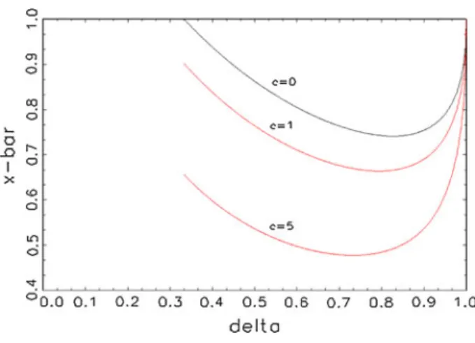
Exploring the comparative statics gives interesting results in the context of marriage. Figure1 shows equilibrium reservation values x as a function of the subjective discount factor d for various values of c. Throughout, we restrict our attention tod C1/3. Interest rates across periods would need to exceed 200% in order for discounting to be so heavy thatd\1/3.15
Given a discount factor, the equilibrium reservation match quality x declines monotonically as the separation cost c rises. Intuitively, higher separation costs mean that players will stay married more easily—a lower reservation valuex:This phenomenon is documented in the literature. Nixon (1997), for example, finds that high child-support payments and stringent enforcement lower the frequency of divorce.
Observe thatxis nonmonotonic in the discount factor, which is a highly unusual game theoretic result. Under most circumstances, possibilities for cooperation increase in a (weakly) monotonic fashion as the discount factor increases: players
Footnote 13 continued
what is presented here is the most profitable possible defection, so guarding against it is sufficient to guard againstanyother type of defection.
14This is obviously a subgame perfect equilibrium since mutual defection is a Nash Equilibrium of the
stage game.
15There is also a technical reason. Discount rates lower than 1/3 do not allow for cooperation using a
are more patient and the future is more important, so cooperation becomes more attractive since the opportunity cost of a one-shot deviation is too high.16 This property holds in our case, but there is an offsetting feature of our model that pulls in the other direction. As d increases and players become more patient, the opportunity cost (discounting) of waiting for a high values ofxfalls, so players are morewilling to divorce their current partners and continue to wait for a partner who generates a better match. People who most easily enter into cooperative marriages are those who are not too impatient, but also not too patient. People who are too impatient overvalue short-term deviations and are not sufficiently deterred by the future threat of divorce; this is standard. On the other hand, people who are too patient do not easily enter into cooperative marriages because they will continue to wait for an extremely good partner. The discounting costs of doing so are low.
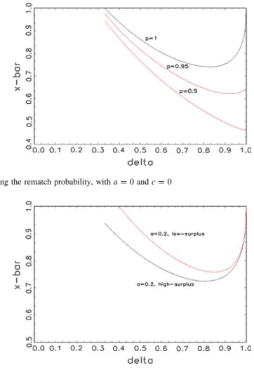
Figure2shows comparative statics in the rematch probabilityp.
Aspdeclines, so too does the reservation marriage qualityx:Again, this makes intuitive sense—if locating a new partner in subsequent periods becomes less likely, then spouses are more inclined to remain in cooperative relationships with their current partners. Different pools of the population are likely to face different prospects upon reentering the marriage market, and the spouses most likely to divorce their current partners are those with the best chance of locating a new match quickly.17 In fact, this effect can become so strong as to swamp the nonmonot-onicity in the discount factor; even for a very patient person, divorcing in hopes of finding a better partner is not optimal if future marriage market prospects are bad. Finally, consider how the allocation of surplus across married partners affects the equilibrium reservation valuex. Recall from our parameterization that the marital
surplus is 4, with share 2?aclaimed by one party and share 2-a by the other.
Fig. 1 Varying the separation cost, witha=0 andp=1
16
Reservation values are also monotonic in the discount factor in the McCall job search model, which is not game-theoretic, but which shares some features with our model.
17Indeed, as one referee pointed out, men tend to marry younger women, so older women may face more
Figures3and4show reservation valuesxfor the high-surplus and the low-surplus partner; Fig.3shows a distribution of the surplus that is more even relative to Fig.4. Everything else equal, the high-surplus partner is more apt to divorce than is the low-surplus partner, assuming that he or she will be able to continue claiming a high share of the surplus for future marriages. Observe that the effect is magnified as the division becomes more unequal. Brinig and Allen (2000) document two empirical regularities that are consistent with this result: college-educated women initiate a higher proportion of divorces than women without college educations, and the proportion of divorces initiated by women generally has been rising over time. If we consider women to be the low-surplus partners, but with the surplus rising as they become more educated and over time generally, these stylized facts are consistent with our result.18
Fig. 3 a=0.2
Fig. 2 Varying the rematch probability, witha=0 andc=0
18Consider pregnancy and asymmetric child-rearing costs, as pointed out by a referee. Another point is
To demonstrate that even the most cooperative possible equilibrium is suboptimal, consider how a benevolent planner would setxto maximize aggregate payoffs. For ease of notation, we consider the case witha=0 and withp=1. The result is qualitatively the same under different parameterizations. If a planner directs a matched couple to continue a cooperative equilibrium, the payoff stream is12xd:If xis too low, the planner will direct that players defect and cease interaction with their current partners, pay the separation cost, then follow the same rule again in the next period. The payoff stream resulting from this defection followed by another (discounted) draw, given thexselected by the planner is:
EVð Þ ¼x 0þd Zx
0
0þdEVð Þ x c
f gdxþ
Z1
x
2x 1d
dx
2 4
3
5: ð11Þ
We can solve (11) to obtain:
EVð Þ ¼x d 1x
2cð1dÞx
1d
ð Þ1d2x
!
ð12Þ
Then a planner will direct players to cooperate perpetually wheneverxsatisfies:
2x 1dd
1x2cð1dÞx
1d
ð Þ1d2x
!
ð13Þ Fig. 4 a=0.5
Footnote 18 continued
Using this parameterization, the equilibrium condition for cooperation, from (9) is: 2x
1d3þd
1x2cð1dÞx 1d
ð Þð1dxÞ
ð14Þ
When checking for equilibrium, one needs to recognize that a playercoulddeviate against a cooperator. Even though players never defect against a cooperative spouse in equilibrium, we need for players’ behavior to be individually rational. A planner, on the other hand, internalizes that in equilibriumbothspouses will defect and so the resulting payoff is 0 rather than 3. He faces no incentive constraint.
Since the left side of (13) is the same as the left side of (14), and the right side of the inequality is greater in (14) than in (13), it follows that the planner will direct mutual cooperation for a lower value ofxthan is possible in equilibrium. That is, there are values ofxfor which it is efficient for players to enter into a mutually cooperative marriage, but for which equilibrium cannot support cooperation. Thex that would maximize aggregate payoffs is lower than the equilibrium value ofx:This model then belongs to a broad class of public-goods provision models where the equilibrium level of provision is inefficiently low. Further, this justifies our claim earlier in this section that equilibria with the lowest possible value ofxwere the most interesting to consider, since the socially optimal value would be still lower.19
4 A dynamic model
We now relax the assumption that each match generates an independent payoff draw regardless of player history. Specifically, each spouse is endowed with a player-specific characteristic that persists across time. As a consequence, the quality of the unmatched pool, and hence the expected value of future matches can change over time. We will consider the simple parameterization, with a=c=0 and with p=1. Other than monotonically providing stronger incentives for cooperation, variations in these parameters do not change the qualitative nature of the results below. The relevant stage game is given in Table3.
As before,x*U[0, 1] is independent upon each new match, and permanent for the duration of lasting matches. However, y1 and y2 are individual-specific and
persistent. Specifically, y is binary. There is some fraction of ‘‘good’’ spouses endowed withy=1 and some fraction of ‘‘bad’’ spouses endowed withy=0. The use of binary player-specific quality follows Ghosh and Ray (1996).20Notice that, if either of the spouses is bad, the cooperative payoff is 0 regardless of the draw ofx. Good players who are matched in this model face even worse prospects from divorce than before: not only does a good spouse face a risk of being matched with a
19
There may be cooperative equilibria with lower reservation values if, for example, the players expect to never remarry. But these change the fundamental nature of the problem, which is repeated access to the same remarriage market.
20
spouse who generates an undesirable value ofx, but he also faces the possibility of being matched with a bad spouse and a payoff of 0 for sure.
The only interesting behavior is among good players who are matched with other good players. Bad players generate cooperative payoffs of 0 regardless of the type of player with whom they are matched, and thus have no incentive to cooperate. We will assume that they defect, divorce and return to the pool each period. That a good spouse will not stay married to a bad spouse is immediate if equilibrium allows for the prospect of cooperation and positive payoffs in the future. We are again interested in reservation equilibria, where a match between two good spouses at timetwill result in perpetual cooperation as long as their draw ofxsatisfiesx[xt:
Here, the reservation value xt is time-indexed since the problem is no longer
stationary: the expected value of being returned to the pool is not the same in each period, since the proportion of good and bad spouses can change over time.
The dynamics are as follows. Throughout, we will letptdesignate the proportion of spousesfrom the unmatched pool (rather than from the population as a whole) who are good at time t. At the beginning of each period, unmatched spouses are matched randomly from the continuum of available spouses.21Some fraction 1 -h
of matches are exogenously destroyed (deaths), and these players are replaced with new entrants, of whom a fractionk are genetically good and a fraction 1-k are genetically bad.22Of proportionhof the matches that survive, proportion 1-ptare
bad players and sopt(1 -pt) is the fraction of good players who were matched with
bad players and will return to the pool. Now, the equilibrium cutoff value ofxfor matched good players isxt;and sincexis uniform on the unit interval, this means
that the probability thatxfalls below xt is exactly xt: Hence, the probability of a
successful match at timetisp2
tð1xtÞ;and the probability that a good player in a
good match is returned to the pool because of an unfavorable draw ofxisp2
txt:We
will replace successful matches with new entrants,23 of whom a fraction k are genetically good and a fraction 1-kare genetically bad. Summarizing, givenpt, there are four types of good spouses in the following period:
Table 3 Stage game for the
dynamic model C D
C 2xy1y2;2xy1y2 1y1y2;3y1y2
D 3y1y2;1y1y2 0;0
21
One might imagine a nonrandom matching process where good spouses are more likely to encounter other good spouses. However, if quality takes time and investment to discover and is not immediately self-evident, then the matching itself may be close to random. Also, as long as there issomepossibility of encountering a bad spouse, and as long as this probability rises when there are more bad spouses in the pool, the salient feature of the matching process for purposes of our model still holds. Also, assortative matching is typically on only one element, so there will always be some hidden information upon matching.
22Notice that the death probability is over matches and not over individuals. In this assumption, we also
follow Ghosh and Ray (1996). It is nonsubstantive in that it does not change the qualitative nature of the results, but it facilitates accounting substantially.
23This keeps the measure of the population at 1. Otherwise, the only steady state would be the trivial one
Description Probability
Genetically good replacements for players in destroyed matches (1-h)k Good players whose matches survived, but who were matched with bad players hpt(1-pt)
Good players whose matches survived, were matched with good players, but had an unfavorable draw ofx
hp2
txt
Genetically good replacements for successful, surviving matches between good players hkp2
tð1xtÞ
Then, since the dynamics are designed to keep the population always at unit mass, Bayes’ rule implies that the population dynamics evolve according to the following difference equation:
ptþ1¼h ptð1ptÞ þpt2xtþkp2tð1xtÞ
þð1hÞk: ð15Þ
Following the logic from earlier, the one-shot deviation principle implies that the incentive constraint for a good player matched with another good player at timetis:
2x
1d3þdhEtþ1½VðxÞ ð16Þ
whereEtþ1½VðxÞis the expected value of being returned to the unmatched pool at
timet?1. To compute this, conditional on an equilibrium valuextþ1 that remains
to be specified24:
Etþ1½VðxÞ ¼ptþ1
Zxtþ1
0
0þdhEtþ2½VðxÞ
f gdxþ
Z1
xtþ1
2x 1ddx 2
6 4
3 7 5
þð1ptþ1Þð0þdhEtþ2½VðxÞÞ ð17Þ
In words, with probabilitypt?1, he will be matched with another good spouse at
timet ?1, and will receive a draw of x. He will receive 0 and be returned to the pool ifx2ð0;xtþ1Þand will receive the discounted value of perpetual cooperation if
x2ðxtþ1;1Þ:With probability 1ptþ1;he will be matched with a bad spouse, will
defect, quit and reenter the pool in the next period. Notice that discounting now incorporates the probability that a match will be destroyed.
The incentive constraint at timetnaturally depends on the expected value of being rematched at timet?1, which depends on the quality of the pool in all future periods. But, the quality of the pool is itself a function of the equilibrium conditions at timetand future periods. As such, we follow Ghosh and Ray and study the steady state of this dynamic system. Here, by steady state, we mean an equilibrium wherept ¼p and
xt¼xfor allt. It follows thatEt½VðxÞ ¼E V½ ðxÞis also constant for allt.25
Imposing the steady state on the expected value computation in (17) allows us to explicitly compute the expected value of being returned to the pool.
24Notice that there is no death within marriage (or alternatively that it is already incorporated into the
discount factor). As in Ghosh and Ray, the death probability given here is interpreted as match destruction.
25While the solution here is for a steady state, as is typical in this literature, the steady state itself cannot
E V½ ðxÞ ¼p Zx
0
0þdhE V½ ðxÞ f gdxþ
Z1
x
2x 1ddx 2
4
3
5þð1pÞð0þdhE V½ ðxÞÞ
ð18Þ )E V½ ðxÞ ¼ p
ð1x2Þ
1d
ð Þð1dhð1pÞ dhpxÞ ð19Þ
Substituting into the incentive constraint gives: 2x
1d3þ
dhpð1x2Þ
1d
ð Þð1dhð1pÞ dhpxÞ ð20Þ
Again, following the logic from earlier in the paper, the lower bound onx(i.e. the equilibrium with the most cooperation) will set the incentive constraint to bind with equality. The proof that this constitutes an equilibrium exactly mimics the parallel proof in section III. Also, we impose steady state conditions on the evolution of the population dynamics in (15). Combining, a steady-state equilibrium vectorðx;pÞ
containing a stationary decision rule and proportion of good players in the unmatched pool satisfies the following two equations:
2x 1d¼3þ
dhpð1x2Þ
1d
ð Þð1dhð1pÞ dhpxÞ ð21Þ p¼h p ð1pÞ þp2xþkp2ð1xÞ þð1hÞk: ð22Þ
Again, this specifies the most cooperative possible steady-state equilibrium. One could specify other equilibria with less cooperation, including the trivial equilibrium with no cooperation.
The table in the appendix gives numerically estimated steady-state equilibrium vectors for various parameter values. The comparative statics have intuitive interpretations in our context. First, decreases inkdecreasex and decreasep:As
the quality of new entrants gets worse, spouses are more likely to stay with their current spouses (a lower value ofx), and clearly the steady state proportion of good spouses decreases as well.26Second, decreases in the match survival probabilityh
decrease x and increase p: As matches are more likely to be exogenously
destroyed, players enter cooperative equilibria with good spouses more readily since there is a higher chance that future matches will be destroyed. However, it increases the steady state proportion of good spouses in the pool since bad spouses are more quickly destroyed and replaced with new births, and in all cases the genetic proportion of good spouses among rebirthskexceeds the equilibrium steady state proportion of good spouses p: Finally, x and p are nonmonotonic in d, first decreasing and then increasing. The logic here is the same as in the static model: as
d increases, the one-shot deviation becomes relatively less attractive, making cooperation more likely. But, the discounting costs of waiting for a better draw of
26This is for two reasons. Players are staying married more easily since the reservation draw ofxis
xare lower, making players more likely to divorce spouses who generate a moderate value ofx. This has an obvious correspondence with the comparative static inp:as
xdecreases, so too does the mean quality of the poolp since good spouses do not return to the pool as frequently.
One feature of the equilibria noted above bears mention: in all cases, the steady state proportion of good spousespis lower than the genetic proportionk. This can be thought of as a kind of adverse selection result. Ifk is thought of as an initial condition on the value of p, then this is unsustainable in equilibrium since the equilibrium p\k always. The equilibrium quality of the pool of unmatched
spouses is worse than the average genetic quality.
5 Conclusion
The dynamics of changing family arrangements deserve attention by economists. This paper addresses the increasingly strong empirical regularity of high turnover in marriage markets (Isen et al. 2008). I have introduced new features to a noncooperative marriage model in order to explicitly incorporate the possibility of remarriage, and shown that there are subgame perfect equilibria that admit perpetual cooperation with a single spouse. The repeated public goods framework extends and adapts the conventional repeated family allocation framework to elucidate the import of allowing for remarriage. Indeed, this model presents the most flexible remarriage setting in the literature. In locating these equilibria, I have shown that, in equilibrium, spouses who most readily enter into cooperative marriages are those with intermediate patience levels. Spouses who are too impatient overvalue short-term deviations against their current partners, but spouses who are too patient also do not readily enter into cooperative marriages since their discounting costs of waiting for an extremely good spouse are low. Low-cost divorce, high rematch probability and the ability to claim a high share of the marital surplus lead to more divorce initiation. I showed that similar equilibria exist in a model allowing for player-specific characteristics that persist across time, presented the dynamics and showed reasonably intuitive comparative statics of the model. In doing so, I have also contributed to a game theory literature studying repeated prisoner’s dilemmas with endogenous exit and have shown that randomness in payoffs presents a new avenue for cooperation not explored by other authors.
One possible extension of this model is to integrate the assortative matching that is common in other models of marriage (e.g. Becker1973). To have any substance, this would require something of higher dimension than binary player type assignments, and then one would introduce correlation between these player types and the matching process: making it more likely that players of certain types would find themselves matched.
A second extension would be to explicitly introduce a probationary dating period where spouses can receive noisy signals about their partners’ qualities. This is similar to the reputations literature between firms and customers.
unexplored. More carefully specifying players’ outside options within the context of marriage can surely inform our evolving understanding of behavior conditional on a cooperative equilibrium having been reached.
Appendix 1: Proof of inequalities (3)–(5) from Sect.3
When each spouse unilaterally maximizes utility, the decision problem from (1) and (2) is:
max
wi;gi
wiþf gi;gj
s:t: wiþPggi¼Yi ð23Þ
Each spousei’s level of contribution to the public good solves:
of
ogi
¼Pg ð24Þ
By contrast, the Pareto optimal collective solution is: max
w1;g1;w2;g2
w1þw2þ2f gi;gj
s:t: w1þw2þPgðg1þg2Þ ¼Y1þY2 ð25Þ
In contrast to (25), the optimal level of contribution to the public good for each spouseisolves:
of
ogi
¼Pg
2 ð26Þ
The concavity of f() implies that public good provision is higher for the (C,C) outcome given in (26) than for the (D,D) outcome given in (24). With this established, the inequality in (3) is trivial since (26) maximizes U1CC?U2CC by
definition, and the solutions in (24) and (26) are distinct. Finally, by definition each spouseialways earns his highest utility for a fixed value ofgjby choosing the level
of contribution given in (24), which establishes the inequalities in (4) and (5).
Appendix 2: Numerical solutions from Sect.4
d=.999 d=.99 d=.9 d=.8 d=.7 d=.6
h=.99
k=.999 x¼:862
p¼:986
x¼:831 p¼:983
x¼:738 p¼:974
x¼:731 p¼:973
x¼:757 p¼:976
x¼:800 p¼:980
k=.99 x¼:855
p¼:879
x¼:819 p¼:858
x¼:711 p¼:805
x¼:704 p¼:802
x¼:735 p¼:815
x¼:786 p¼:840
k=.9 x¼:807
p¼:473
x¼:752 p¼:435
x¼:587 p¼:362
x¼:588 p¼:363
x¼:644 p¼:383
x¼:725 p¼:420
k=.8 x¼:772
p¼:324
x¼:706 p¼:295
x¼:520 p¼:242
x¼:533 p¼:245
x¼:602 p¼:262
Appendix continued
d=.999 d=.99 d=.9 d=.8 d=.7 d=.6
k=.5 x¼:683
p¼:149
x¼:676 p¼:233
x¼:401 p¼:114
x¼:444 p¼:118
x¼:540 p¼:127
x¼:656 p¼:145
d=.999 d=.99 d=.9 d=.8 d=.7 d=.6
h=.9
k=.999 x¼:626
p¼:996
x¼:627 p¼:996
x¼:645 p¼:996
x¼:679 p¼:996
x¼:725 p¼:997
x¼:781 p¼:997
k=.99 x¼:621
p¼:959
x¼:621 p¼:959
x¼:639 p¼:960
x¼:674 p¼:963
x¼:721 p¼:967
x¼:779 p¼:971
k=.9 x¼:575
p¼:708
x¼:575 p¼:708
x¼:591 p¼:713
x¼:632 p¼:726
x¼:689 p¼:745
x¼:758 p¼:771
k=.8 x¼:534
p¼:548
x¼:534 p¼:548
x¼:549 p¼:552
x¼:596 p¼:566
x¼:661 p¼:588
x¼:739 p¼:620
k=.5 x¼:426
p¼:287
x¼:424 p¼:287
x¼:444 p¼:290
x¼:508 p¼:300
x¼:593 p¼:317
x¼:693 p¼:340
References
Andaluz, J., & Molina, J. A. (2007). On the sustainability of bargaining solutions in family decision models.Review of Economics of the Household, 5, 405–418.
Becker, G. S. (1973). A theory of marriage: Part I.The Journal of Political Economy, 81, 813–846. Becker, G. S. (1981).A treatise on the family. Cambridge: Harvard University Press.
Bourguignon, F., Browning, M., Cciappori, P.-A., & Lechene, V. (1993). Intra-household allocation of consumption: A model and some evidence from french data.Annales d’Economie et de Statistique, 29, 138–156.
Brinig, M., & Allen, D. (2000). These boots are made for walking: Why most divorce filers are women. American Law and Economics Review, 2, 126–129.
Carmichael, L., & Macleod, B. (1997). Gift giving and the evolution of cooperation.International Economic Review, 38, 485–510.
Chiappori, P.-A, Iyigun, M., & Weiss, Y. (2009). Spousal matching with children, careers and divorce. Working paper.
Chiappori, P.-A, Iyigun, M., & Weiss, Y. (2009). Divorce laws, remarriage and spousal welfare. Working paper.
Chiappori, P.-A., & Weiss, Y. (2006). Divorce, remarriage and welfare: A general equilibrium approach. Journal of the European Economic Association, 4, 415–426.
Datta, S. (1996). Building trust. STICERD Theoretical Economics Paper Series.
Flinn, C. J. (2000). Models of interaction between divorced parents.International Economic Review, 41, 545–578.
Ghosh, P., & Ray, D. (1996). Cooperation in community interactions without information flows.Review of Economic Studies, 63, 491–519.
Hoddinott, J., & Adam, C. (1998). Testing nash bargaining household models with time series data. Food Consumption and Nutrition Division.
Isen, A., & Stevenson, B. (2008). Women’s education and family behavior: Trends in marriage, divorce and fertility. Working paper.
Iyigun, M., & Walsh, R. P. (2007). Building the family nest: Pre-marital investments, marriage markets and spousal allocations.Review of Economic Studies, 74, 507–535.
Konrad, K. A., & Lommerud, K. E. (1995). Family policy with non-cooperative families. The Scandinavian Journal of Economics, 97, 581–601.
Lundberg, S., & Pollak, R. A. (1994). Noncooperative bargaining models of marriage.The American Economic Review, 84, 132–137.
Lundberg, S., & Pollak, R. A. (2003). Efficiency in marriage.Review of Economics of the Household, 1, 153–168.
Lundberg, S., & Pollak, R. A. (2007). The American family and family economics.Journal of Economic Perspectives, 21, 3–26.
Mailath, G. J., & Samuelson, L. (2006).Repeated games and reputations. New York: Oxford University Press.
Manser, M., & Brown, M. (1980). Marriage and household decision making: A bargaining analysis. International Economic Review, 21, 31–44.
McCall, J. J. (1970). Economics of information and job search.The Quarterly Journal of Economics, 84, 113–126.
Nixon, L. (1997). The effect of child support enforcement on marital dissolution.The Journal of Human Resources, 32, 159–181.
Schluessler, R. (1989). Exit threats and cooperation under anonymity.Journal of Conflict Resolution, 33, 728–749.
Stevenson, B. (2007). The impact of divorce laws on marriage-specific capital. Journal of Labor Economics, 25, 75–94.
Stevenson, B., & Wolfers, J. (2007). Marriage and divorce: Changes and their driving forces.Journal of Economic Perspectives, 21, 27–52.
Tauchen, H. V., Witte, A. D., & Long, S. K. (1991). Domestic violence: A nonrandom affair. International Economic Review, 32, 491–511.
Ulph, D. (1988).A general noncooperative nash model of household behaviour. Mimeo: University of Bristol.