Introduction to Stacks and Moduli

(1)

Introduction to Stacks and Moduli

Lecture notes for Math 582D,

working draft

University of Washington, Winter 2021

Jarod Alper

[email protected]

January 5, 2021

(2)

(3)

Abstract

These notes provide the foundations of moduli theory in algebraic geometry using the language of algebraic stacks with the goal of providing a self-contained proof of the following theorem:

Theorem A. The moduli space Mg of stable curves of genus g≥2 is a smooth, proper and irreducible Deligne–Mumford stack of dimension3g−3which admits a projective coarse moduli space.1

Along the way we develop the foundations of algebraic spaces and stacks, and we hope to convey that this provides a convenient language to establish geometric properties of moduli spaces. Introducing these foundations requires developing several themes at the same time including:

• using the functorial and groupoid perspective in algebraic geometry: we will introduce the new algebro-geometric structures of algebraic spaces and stacks;

• replacing the Zariski topology on a scheme with the ´etale topology: we will generalize the concept of a topological space to Grothendieck topologies and systematically using descent theory for ´etale morphisms; and

• relying on several advanced topics not seen in a first algebraic geometry course: properties of flat, ´etale and smooth morphisms of schemes, algebraic groups and their actions, deformation theory, Artin approximation, existence of Hilbert schemes, and some deep results in birational geometry of surfaces. Choosing a linear order in presenting the foundations is no easy task. We attempt to mitigate this challenge by relegating much of the background to appendices. We keep the main body of the notes always focused entirely on developing moduli theory with the above goal in mind.

1_{In a future course, I hope to establish an analogous result for the moduli of vector bundles:} The moduli spaceMss

C,r,d of semistable vector bundles of rankrand degreedover a smooth,

connected and projective curveC of genusgis a smooth, universally closed and irreducible algebraic stack of dimensionr2₍_g₋_{1) which admits a projective good moduli space.}

(4)

(5)

Introduction and motivation

Amoduli spaceis a spaceM (e.g. topological space, complex manifold or algebraic variety) where there is a natural one-to-one correspondence between points ofM

and isomorphism classes of certain types of algebro-geometric objects (e.g. smooth curves or vector bundles on a fixed curve). While any spaceM is the moduli space parameterizing points ofM, it is much more interesting when alternative descriptions can be provided. For instance, projective space_P1_{can be described}

as the set of points inP1 (not so interesting) or as the set of lines in the plane

passing through the origin (more interesting).

Moduli spaces arise as an attempt to answer one of the most fundamental problems in mathematics, namely the classification problem. In algebraic geometry, we may wish to classify all projective varieties, all vector bundles on a fixed variety or any number of other structures. The moduli space itself is the solution to the classification problem.

Depending on what objects are being parameterized, the moduli space could be discrete or continuous, or a combination of the two. For instance, the moduli space parameterizing line bundles on_P1_{is the discrete set}

Z: every line bundle

on_P1_{is isomorphic to} _O₍_n_{) for a unique integer}_n_∈

Z. On the other hand, the

moduli space parameterizing quadric plane curveC⊂_P2_{is the connected space}

P5: a plane curve defined by a0x2+a1xy+a2xz+a3y2+a4yz+a5z2 is uniquely

determined by the point [a0, . . . , a5]∈P5, and as a plane curve varies continuously

(i.e. by varying the coefficientsai), the corresponding point inP5 does too.

The moduli space parameterizing smooth projective abstract curves has both a discrete and continuous component. While the genus of a smooth curve is a discrete invariant, smooth curves of a fixed genus vary continuously. For instance, varying the coefficients of a homogeneous degreedpolynomial inx, y, zdescribes a continuous family of mostly non-isomorphic curves of genus (d−1)(d−2)/2. After fixing the genusg, the moduli spaceMg parameterizing genusg curves is a

connected (even irreducible) variety of dimension 3g−3, a deep fact providing the underlying motivation of these notes. Similarly, the moduli space of vector bundles on a fixed curve has a discrete component corresponding to the rankrand degreedof the vector bundle, and it turns out that after fixing these invariants, the moduli space is also irreducible.

An inspiring feature of moduli spaces and one reason they garner so much attention is that their properties inform us about the properties of the objects themselves that are being classified. For instance, knowing thatMg is unirational

(8)

(i.e. there is a dominant rational map_PN

99KMg) for a given genusgtells us that

a general genusg curve can be written down explicitly in a similar way to how a general genus 3 curve can be expressed as the solution set to a plane quartic whose coefficients are general complex numbers.

Before we can get started discussing the geometry of moduli spaces such as

Mg, we need to ask: why do they even exist? We develop the foundations of

moduli theory with this single question in mind. Our goal is to establish the truly spectacular result that there is a projective variety whose points are in natural one-to-one correspondence with isomorphism classes of curves (or vector bundles on a fixed curve). In this chapter, we motivate our approach for constructing projective moduli spaces through the language of algebraic stacks.

0.1 Moduli sets

Amoduli setis a set where elements correspond to isomorphism classes of certain types of algebraic, geometric or topological objects. To be more explicit, defining a moduli set entails specifying two things:

1. a class of certain types of objects, and 2. an equivalence relation on objects.

The word ‘moduli’ indicates that we are viewing an element of the set of as an equivalence class of certain objects. In the same vein, we will discuss moduli groupoids,moduli varieties/schemesandmoduli stacksin the forthcoming sections. Meanwhile, the word ‘object’ here is intentionally vague as the possibilities are quite broad: one may wish to discuss the moduli of really any type of mathematical structure, e.g. complex structures on a fixed space, flat connections, quiver representations, solutions to PDEs, or instantons. In these notes, we will entirely focus our study on moduli problems appearing in algebraic geometry although many of the ideas we present extend similarly to other branches of mathematics. The two central examples in these notes are the moduli of curves and the moduli of vector bundles on a fixed curve—two of the most famous and studied moduli spaces in algebraic geometry. While there are simpler examples such as projective space and the Grassmanian that we will study first, the moduli spaces of curves and vector bundles are both complicated enough to reveal many general phenomena of moduli and simple enough that we can provide a self-contained exposition. Certainly, before you hope to study moduli of higher dimensional varieties or moduli of complexes on a surface, you better have mastered these examples.

0.1.1 Moduli of curves

Here’s our first attempt at definingMg:

Example 0.1.1(Moduli set of smooth curves). Themoduli set of smooth curves, denoted asMg, is defined as followed: the objects are smooth, connected and

projective curves of genus g over C and the equivalence relation is given by

isomorphism.

There are alternative descriptions. We could take the objects to be complex structures on a fixed oriented compact surface Σ of genusg and the equivalence relation to be biholomorphism. Or we could take the objects to be pairs (X, φ)

(9)

whereXis a hyberbolic surface andφ: Σ→X is a diffeomorphism (the set of such pairs is the Teichm¨uller space) and the equivalence relation is isotopy (induced from the action of the mapping class group of Σ).

Each description hints at different additional structures thatMgshould inherit.

There are many related examples parameterizing curves with additional struc-tures as well as different choices for the equivalences relations.

Example 0.1.2(Moduli set of plane curves). The objects here are degreedplane curvesC⊂P2 but there are several choices for how we could define two plane

curvesC andC0 _{to be equivalent:}

(1) C andC0 are equal as subschemes;

(2) C andC0 are projectively equivalent (i.e. there is an automorphism of_P2

takingC toC0); or

(3) C andC0 are abstractly isomorphic.

The three equivalence relations define three different moduli sets. The moduli set

(1)is naturally bijective to the projectivization P(SymdC3) of the space of degree

dhomogeneous polynomials inx, y, zwhile the moduli set(2)is naturally bijective to the quotient setP(SymdC3)/Aut(P2). The moduli set(3)is the subset of the

moduli set of (possibly singular) abstract curves which admit planar embeddings. Example 0.1.3(Moduli set of curves with leveln structure). The objects are smooth, connected and projective curves C of genus g over _Ctogether with a basis (α1, . . . , αg, β1, . . . , βg) of H1(C,Z/nZ) such that the intersection pairing

is symplectic. We say that (C, αi, βi) ∼(C0, α0i, βi0) if there is an isomorphism

C→C0 takingαi andβi toα0i andβi0.

A rational functionf /g on a curve C defines a map C →_P1 _{given by} _x_7→

[f(x), g(x)]. Visualizing a curve as a cover of_P1_{is extremely instructive providing}

a handle to its geometry. Likewise it is instructive to consider the moduli of such covers.

Example 0.1.4 (Moduli of branched covers). We define theHurwitz moduli set

Hurd,g where an object is a smooth, connected and projective curve of genus

g together with a finite morphisms f: C → _P1 _{of degree} _d_{, and we declare}

(C −→f P1) ∼ (C0 f

0

−→ P1) if there is an isomorphism α: C → C0 over P1 (i.e.

f0 = f ◦α). By Riemann–Hurwitz, any such map C → P1 has 2d+ 2g−2

branch points. Conversely, given a general collection of 2d+ 2g−2 points ofP1,

there exists a genusg curveC and a mapC→P1 branched over precisely these

points. In fact there are only finitely many such coversC→P1 as any cover is

uniquely determined by the ramification type over the branched points and the finite number of permutations specifying how the unramified covering over the complement of the branched locus is obtained by gluing trivial coverings. In other words, the map Hurd,g→Sym2d+2g−2P1, assigning a cover to its branched points,

has dense image and finite fibers.

Likewise, for a fixed curve C, we could consider the moduli set Hurd,C

pa-rameterizing degreedcovers C→_P1 _{where the equivalence relation is equality.}

There is a map Hurd,g → Mg defined by (C → P1) 7→C, and the fiber over a

curveC is precisely Hurd,C. Equivalently, Hurd,C can be described as

parame-terizing line bundlesL on C together with linearly independent sections s1, s2

where (L, s1, s2)∼(L0, s10, s02) if there exists an isomorphism α:L→L0 such that

(10)

Application: number of moduli ofMg

Even before we attempt to giveMg the structure of a variety so that in particular

its dimension makes sense, forg≥2 we can use a parameter count to determine thenumber of moduli of Mg or in modern terminology thedimension of the local deformation spaces. Historically Riemann computed the number of moduli in the mid 19th century (in fact using several different methods) well before it was known thatMg is a variety. Following [Rie57], the main idea is to compute the

number of moduli of Hurd,gin two different ways using the diagram

Hurd,C //

{

Hurd,g

z

finite fibers

&

{C} ////Mg Sym2d+2g−2P1

(0.1.1)

We first compute the number of moduli of Hurd,C and we might as well assume

thatdis sufficiently large (or explicitlyd >2g). For a fixed curveC, a degreedmap

f:C→P1 is determined by an effective divisorD:=f−1(0) =Pipi∈SymdC

and a sectiont∈H0(C,O(D)) (so that f(p) = [s(p), t(p)] where s∈Γ(C,O(D)) definesD). Using thatH1₍_C,_O₍_D_{)) =}_H0₍_C,_O₍_K

C−D)) = 0, Riemann–Roch

implies thath0₍_O₍_D_{)) =}_d₋_g_{+ 1. Thus the number of moduli of Hur}

d,C is the

sum of the number of parameters determiningD and the sectiont

# of moduli of Hurd,C =d+ (d−g+ 1) = 2d−g+ 1.

Using (0.1.1), we compute that

# of moduli ofMg = # of moduli of Hurd,g−# of moduli of Hurd,C

= # of moduli of Sym2d+2g−2P1−# of moduli of Hurd,C

= (2d+ 2g−2)−(2d−g+ 1) = 3g−3.

One goal of these notes is to put this calculation on a more solid footing. The interested reader may wish to consult [GH78, pg. 255-257] or [Mir95, pg. 211-215] for further discussion on the number of moduli ofMg, or [AJP16] for a historical

background of Riemann’s computations.

0.1.2 Moduli of vector bundles

The moduli of vector bundles on a fixed curve provides our second primary example of a moduli set:

Example 0.1.5 (Moduli set of vector bundles on a curve). Let C be a fixed smooth, connected and projective curve over_C, and fix integersr≥0 andd. The objects of interest are vector bundles E (i.e. locally free OC-modules of finite

rank) of rankr and degreed, and the equivalence relation is isomorphism. There are alternative descriptions. If V is a fixed C∞-vector bundleV on

C, we can take the objects to be connections on V and the equivalence relation to be gauge equivalence. Or we can take the objects to be representations

π1(C)→GLn(C) of the fundamental groupπ1(C) and declare two representations

(11)

element of GLn(C). This last description uses the observation that a vector bundle

induces a monodromy representation ofπ1(C) and conversely that a representation

V ofπ1(C) induces a vector bundle (Ce×V)/π1(C) onC, whereCe denotes the

universal cover ofC.

Specializing to the rank one case is a model for the general case: the moduli set Picd(C) of line bundles onCof degreedis identified (non-canonically) with the abelian variety H1₍_C,_O

C)/H1(C,Z) by means of the cohomology of the

exponential exact sequence

H1₍_C,

Z) //H1(C,OC) //Pic(C)

L7→deg(L)

/

/H2₍_C,

Z) //0

There is a group structure on Pic0(C) corresponding to the tensor product of line bundles.

Example 0.1.6(Moduli of vector bundles on P1). Since all vector bundles on A1 are trivial, a vector bundle of rank n on P1 is described by an element of

GLn(k[x]x) specifying how trivial vector bundles on{x 6= 0} and{y 6= 0} are

glued. We can thus describe this moduli set by taking the objects to be elements of GLn(k[x]x) where two elementsg andg0 are declared equivalent if there exists

α∈ GLn(k[x]) andβ ∈ GLn(k[1/x]) (i.e. automorphisms of the trivial vector

bundles on{x6= 0}and{y6= 0}) such thatg0=αgβ.

The Birkhoff–Grothendieck theorem asserts that any vector bundleEon _P1_is

isomorphic toO(a1)⊕ · · · ⊕O(ar) for unique integersa1≤ · · · ≤ar.1 This implies

that the moduli set of degreedvector bundles of rankr onP1 is bijective to the

set of increasing tuples (a1, . . . , ar)∈Zr of integers withPiai=d. One would

be mistaken though to think that the moduli space of vector bundles onP1with

fixed rank and degree is discrete. For instance, ifd= 0 andr= 2, the group of extensions

Ext1(O_P1(1),O_P1(−1)) =H1(_P1,O_P1(−2)) =H0(_P1,O_P1) =_C

is one-dimensional and the universal extension (seeExample 0.4.21) is a vector bundleE on P1×A1 such that E|P1×{t} is the non-trivial extension OP1⊕OP1

fort6= 0 and the trivial extensionO_P1(−1)⊕O_P1(1) fort= 0. This shows that

OP1⊕OP1 andOP1(−1)⊕OP1(1) should be in the same connected component of

the moduli space.

0.1.3 Wait—why are we just defining sets?

It is indeed a bit silly to define these moduli spaces as sets. After all, any two complex projective varieties are bijective so we should be demanding a lot more structure than a variety whose points are in bijective correspondence with isomorphism classes. However, spelling out what properties we desire of the moduli space is by no means easy. What we would really like is a quasi-projective variety 1_{Birkhoff proved this in 1909 using linear algebra by explicitly showing that an element} GLn(k[x]x) can be multiplied on the left and right by elements of GLn(k[x]) and GLn(k[1/x])

to be a diagonal matrix diag(xa1_{, . . . , x}ar_{) [}_Bir09_{] while Grothendieck proved this in 1957 via} induction and cohomology by exhibiting a line subbundleO(a)⊂Esuch that the corresponding short exact sequence splits [Gro57].

(12)

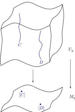
Mg with a universal familyUg→Mgsuch that the fiber of a point [C]∈Mg is

precisely that curve. This is where the difficulty lies—automorphisms of curves obstruct the existence of such a family—and this is the main reason we want to expand our notion of a geometric space from schemes to algebraic stacks. Algebraic stacks provide a nice approach ensuring the existence of a universal family but it is by no means the only approach.

Historically, it was not clear what structure Mg should have. Riemann

in-troduced the word ‘Mannigfaltigkeiten’ (or ‘manifoldness’) but did not specify what this means–complex manifolds were only introduced in the 1940s following Teichm¨uller, Chern and Weil. The first claim thatMgexists as an algebraic variety

was perhaps due to Weil in [Wei58]: “As forMg there is virtually no doubt that it

can be provided with the structure of an algebraic variety.” Grothendieck, aware that the functor of smooth families of curves was not representable, studied the functor of smooth families of curves with level structurer≥3 [Gro61]. While he could show representability, he struggled to show quasi-projectivity. It was only later that Mumford proved thatMg is a quasi-projective variety, an

accomplish-ment for which he was awarded the Field Medal in 1974, by introducing and then applying Geometric Invariant Theory (GIT) to constructMg as a quotient [GIT].

For further historical background, we recommend [JP13], [AJP16] and [Kol18].

In these notes, we take a similar approach to Mumford’s original construction and integrate later influential results due to Deligne, Koll´ar, Mumford and others such as the seminal paper [DM69] which simultaneously introduced stable curves and stacks with the application of irreducibility ofMgin any characteristic. In this

chapter, we motivate our approach by gradually building in additional structure: first as a groupoid (Section 0.3), then as a presheaf (i.e. contravariant functor) (Section 0.4), then as a stack (Section 0.7) and then ultimately as a projective variety (Section 0.9).

One of the challenges of learning moduli stacks is that it requires simultaneously extending the theory of schemes in several orthogonal directions including:

(1) the functorial approach: thinking of a schemeX not as topological space with a sheaf of rings but rather in terms of the functor Sch→Sets defined by T 7→Mor(T, X). For moduli problems, this means specifying not just objects but families of objects; and

(2) the groupoid approach: rather than specifying just the points we also specify their symmetries. For moduli problems, this means specifying not just the objects but their automorphism groups.

(13)

Sets

Topological spaces

Functors or presheaves on Sch

Ringed spaces

Schemes Algebraic spaces Sheaves on Sch´Et

Groupoids

Prestacks over Sch

Stacks over SchEt´

Deligne–Mumford stacks

Algebraic stacks

Figure 1: Schematic diagram featuring algebro-geometric enrichments of sets and groupoids where arrows indicate additional geometric conditions.

0.2 Toy example: moduli of triangles

Before we dive deeper into the moduli of curves or vector bundles, we will study the simple yet surprisingly fruitful example of the moduli of triangles which is easy both to visualize and construct. In fact, we present several variants of the moduli of triangles that highlight various concepts in moduli theory. The moduli spaces of labelled triangles and labelled triangles up to similarity have natural functorial descriptions and universal families while the moduli space ofunlabelled triangles does not admit a universal family due to the presence of symmetries—in exploring this example, we are led to the concept of a moduli groupoid and ultimately to moduli stacks. Michael Artin is attributed to remarking that you can understand most concepts in moduli through the moduli space of triangles.

0.2.1 Labelled triangles

Alabelled triangleis a triangle inR2where the vertices are labelled with ‘1’, ‘2’

and ‘3’, and the distances of the edges are denoted asa,b, andc. We require that triangles have non-zero area or equivalently that their vertices are not colinear.

1 2

3

a

b

c

Figure 2: To keep track of the labelling, we color the edges as above.

We define themoduli set of labelled trianglesM as the set of labelled triangles where two triangles are said to be equivalent if they are the same triangle inR2

(14)

as the coordinates of the labelled vertices, we obtain a bijection

M ∼=(x1, y1, x2, y2, x3, y3) | det

x2−x1 x3−x1

y2−y1 y3−y1

6

= 0 ⊂R6 (0.2.1)

with the open subset of_R6 _{whose complement is the codimension 1 closed subset}

defined by the condition that the vectors (x2, y2)−(x1, y1) and (x3, y3)−(x1, y1)

are linearly dependent.

y3

x3

Figure 3: Picture of the slice of the moduli spaceM where (x1, y1) = (0,0) and

(x2, y2) = (1,0). Triangles are described by their third vertex (x3, y3) withy36= 0.

We’ve drawn representative triangles for a handful of points in thex3y3−plane.

0.2.2 Labelled triangles up to similarity

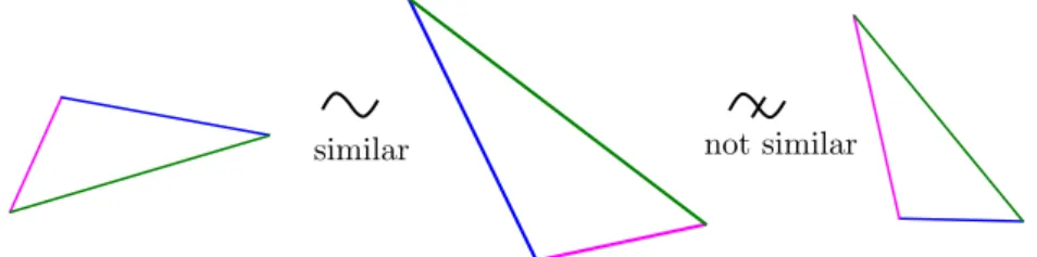
We define themoduli set of labelled triangles up to similarity, denoted byMlab, by taking the same class of objects as in the previous example—labelled triangles—but changing the equivalence relation to label-preserving similarity.

similar not similar

Figure 4: The two triangles on the left are similar, but the third is not. Every labelled triangle is similar to a unique labelled triangle with perimeter

a+b+c= 2. We have the description

Mlab=

   

  

(a, b, c)

a+b+c= 2 0< a < b+c

0< b < a+c

0< c < a+b

   

  

. (0.2.2)

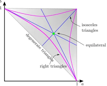
By settingc= 2−a−b, we may visualizeMlab_{as the analytic open subset of}

R2

(15)

a b

degenerate

triangles

right triangles

isosceles triangles

equilateral 1

1

Figure 5: Mlab _{is the shaded area above. The pink lines represent the right}

triangles defined bya2₊_b2 ₌_c2_,_a2₊_c2₌_b2 _and_b2₊_c2 ₌_a2_{, the blue lines}

represent isosceles triangles defined bya=b,b=canda=c, and the green point is the unique equilateral triangle defined bya=b=c.

0.2.3 Unlabelled triangles up to similarity

We now turn to the moduli of unlabelled triangles up to similarity, which reveals a new feature not seen in to the two above examples: symmetry!

We define themoduli set of unlabelled triangles up to similarity, denoted by

Munl_{, where the objects are unlabelled triangles in}

R2and the equivalence relation

is symmetry. We can describe a unlabelled triangle uniquely by the ordered tuple (a, b, c) of increasing side lengths as follows:

Munl=

(a, b, c)

0< a≤b≤c < a+b a+b+c= 2

. (0.2.3)

a b

1

degenerate

a

+

b₌ c

isosceles

a= b

isosceles

b₌

c _equilateral

right triangles

a2₊_b2₌_c2

1/2

1/2 2/3 2/3

(16)

The isosceles triangles witha=b orb=cand the equilateral triangle with

a=b=chave symmetry groups of_Z/2 andS3, respectively. This is unfortunately

not encoded into our description Munl _{above. However, we can identify} _Munl

as the quotientMlab_/S

3 of the moduli set of labelled triangles up to similarity

modulo the natural action ofS3on the labellings. Under this action, the stabilizers

of isosceles and equilateral triangles are precisely their symmetry groupsZ/2 and

S3. The action of S3 on the complement of the set of isosceles and equilateral

triangles is free.

0.3 Moduli groupoids

We now change our perspective: rather than specifying when two objects are identified, we specifyhow! One of the most desirable properties of a moduli space is the existence of a universal family (see§0.4.5) and the presence of automorphisms obstructs its existence (see§0.4.6). Encoding automorphisms into our descriptions will allow us to get around this problem. A convenient mathematical structure to encode this information is agroupoid.

Definition 0.3.1. A groupoidis a category Cwhere every morphism is an iso-morphism.

0.3.1 Specifying a moduli groupoid

Amoduli groupoid is described by

1. a class of certain algebraic, geometric or topological objects; and 2. a set of equivalences between two objects.

where (1) describes the objects and (2) the morphisms of a groupoid. In particular, the moduli groupoid encodes Aut(E) for every objectE.

We say that two groupoidsC1 andC2 areequivalentif there is an equivalence of categories (i.e. a fully faithful and essentially surjective functor) C1 → C2. Moreover, we say that a groupoidCis equivalent to a setΣ if there is an equivalence of categoriesC→CΣ(whereCΣis defined inExample 0.3.2).

0.3.2 Examples

We will return to our two main examples—curves and vector bundles—in a moment but it will be useful first to consider a number a simpler examples.

Example 0.3.2. If Σ is a set, the category CΣ, whose objects are elements of Σ and whose morphisms consist of only the identity morphism, is a groupoid. Example 0.3.3. If Gis a group, theclassifying groupoidBG ofG, defined as the category with one object? such that Mor(?, ?) =G, is a groupoid.

Example 0.3.4. The category FB of finite sets where morphisms are bijections is a groupoid. Observe that the isomorphism classes of FB are in bijection with_N but the groupoid FB retains the information of the permutation groupsSn.

Example 0.3.5 (Projective space). Projective space can be defined as a moduli groupoid where the objects are lines L ⊂An+1 through the origin and whose

(17)

non-zero linear mapsx= (x0, . . . , xn) :C→ Cn+1 such that there is a unique

morphismx→x0 if im(x) = im(x0)⊂_Cn+1 _{(i.e. there exists a} _λ_∈

C∗ such that

x0=λx) and no morphisms otherwise.

0.3.3 Moduli groupoid of orbits

Example 0.3.6 (Moduli groupoid of orbits). Given an action of a groupGon a setX, we define themoduli groupoid of orbits[X/G]2 _{by taking the objects to be} all elementsx∈X and by declaring Mor(x, x0) ={g∈G|x0=gx}.

[_A1_/₍

Z/2)] A1

Z/2

A1

[A1/Gm]

Gm {1}

0

Figure 7: Pictures of the scaling actions of_Z/2 ={±1}and_GmonA1overCwith

the automorphism groups listed in blue. Note that [_A1_/

Gm] has two isomorphism

classes of objects—0 and 1—corresponding to the two orbits—0 and_A1_\_0—such

that 0∈ {1}if the set_A1_/

Gm is endowed with the quotient topology.

Exercise 0.3.7.

(1) Show that the moduli groupoid of orbits [X/G] inExample 0.3.6is equivalent to a set if and only if the action ofGonX is free.

(2) Show that a groupoid C is equivalent to a set if and only ifC→C×Cis fully faithful.

Example 0.3.8. Consider the categoryCwith two objectsx1 andx2such that

Mor(xi, xj) ={±1} for i, j = 1,2 where composition of morphisms is given by

multiplication. ThenCis equivalentBZ/2.

1 -1

x1

1 -1

x2

1 -1

x

xi x

Figure 8: An equivalence of groupoids

Exercise 0.3.9. InExample 0.3.8, show that there is an equivalence of categories inducing a bijection on objects betweenCand either [(Z/2)/(Z/4)] or [(Z/2)/(Z/2× Z/2)] where the action is given by the surjectionsZ/4→Z/2 orZ/2×Z/2→Z/2.

2_{We use brackets to distinguish the groupoid quotient [}_X/G_{] from the set quotient} _X/G_. Later whenGandX are enriched with more structure (e.g. an algebraic group acting on a variety), then [X/G] will be correspondingly enriched (e.g. as an algebraic stack).

(18)

Example 0.3.10 (Projective space as a quotient). The moduli groupoid of projective space (Example 0.3.5) can also be described as the moduli groupoid of orbits [(An+1\0)/Gm].

We can also consider the quotient groupoid [_An+1_/

Gm], which is equivalent to

the groupoid whose objects are (possibly zero) linear mapsx= (x0, . . . , xn) :C→ Cn+1 such that Mor(x, x0) ={t∈C∗|x0i=txi for alli}. We can thus viewPn as

a subgroupoid of [_An+1_/

Gm].

Exercise 0.3.11. If a groupGacts on a set X andx∈X is any point, there exists a fully faithful functorBGx→[X/G]. If the action is transitive, show that

it is an equivalence.

A morphisms of groupoids C1 →C2 is simply a functor, and we define the category MOR(C1,C2) whose objects are functors and whose morphisms are natural transformations.

Exercise 0.3.12. If C1 and C2 are groupoids, show that MOR(C1,C2) is a groupoid.

Exercise 0.3.13. IfH andGare groups, show that there is an equivalence

MOR(BH, BG) = G

φ∈Conj(H,G)

BNG(imφ)

where Conj(H, G) denotes a set of representatives of homomorphismsH →Gup to conjugation byG, and NG(imφ) denotes the normalizer of imφinG.

Exercise 0.3.14. Provide an example of group actions ofH andGon sets X

andY and a map [X/H]→[Y /G] of groupoids thatdoes notarise from a group homomorphismφ:H →Gand aφ-equivariant mapX→Y.

0.3.4 Moduli groupoids of curves and vector bundles

We return to the two main examples in these notes.

Example 0.3.15(Moduli groupoid of smooth curves). In this case, the objects are smooth, connected and projective curves of genusg over_Cand for two curves

C, C0, the set of morphisms is defined as the set of isomorphisms Mor(C, C0) ={isomorphismsα:C→∼ C0}.

Example 0.3.16 (Moduli groupoid of vector bundles on a curve). Let C be a fixed smooth, connected and projective curve over_C, and fix integersr≥0 andd. The objects are vector bundlesE of rankrand degreed, and the morphisms are isomorphisms of vector bundles.

0.3.5 Moduli groupoid of unlabelled triangles up to

simi-larity

We now revisit Section 0.2.3 of the moduli set Munl _{of unlabelled triangles}

up to similarity. We will show later that this moduli set does not admit a natural functorial descriptions nor universal family due to presence of symmetries

(19)

(Example 0.4.37). Since these are such desirable properties, we will pursue a work around where we encode the symmetries into the definition.

We define themoduli groupoid of unlabelled triangles up to similarity, denoted byMunl_{(note the calligraphic font), where the objects are unlabelled triangles}

in_R2 _{and where for triangles} _T

1, T2 ⊂ R2, the set Mor(T1, T2) consists of the

symmetriesσ(corresponding to the permutations of the vertices) such thatT1is

similar toσ(T2). For example, an isosceles triangle (resp. equilateral triangle) has

automorphism groupZ/2 (resp. S3).

We can draw essentially the same picture as Figure 6 except we mark the automorphisms of triangles.

a b

1

a

+

b

=

c

a= b b₌

c

equilateral

a2₊_b2₌_c2

S3

Z₂

Z2 1/2

1/2 2/3

2/3

Figure 9: Picture of the moduli groupoidMunl _{with non-trivial automorphism}

groups labelled. There is a functor

Munl_→_Munl

which is the identity on objects and collapses all morphisms to the identity. This could be called acoarse moduli setwhere by forgetting some information (i.e. the symmetry groups of isosceles and equilateral triangles), we can study the moduli problem as a more familiar object (i.e. a set rather than groupoid).

Exercise 0.3.17. Recall that the moduli set Mlab of labelled triangles up to similarity has the description as the set of tuples (a, b, c) such thata+b+c= 2, 0< a < b+c, 0< b < a+c, and 0< c < a+b (see from (0.2.1) ) Show that there is a natural action ofS3 on the moduli setMlab of unlabelled triangles up

to similarity and that the functor obtained by forgetting the labelling [Mlab/S3]→Munl

is an equivalence of categories.

Exercise 0.3.18. Define a moduli groupoid oforiented trianglesand investigate its relation to the moduli sets and groupoids of triangles we’ve defined above.

(20)

0.4 Moduli functors

We now undertake the challenging task of motivating moduli functors, which will be our approach for endowing moduli sets with the enriched structure of a topological space or scheme. This will require a leap in abstraction that is not at all the most intuitive, especially if you are seeing for the first time. The idea due to Grothendieck is to study a schemeX by studying all maps to it!

It may seem that this leap made life more difficult for us: rather than just specifying the points of a moduli space, we need to define all maps to the moduli space. In fact, it is easier than you may expect. Let’s takeMg as an example.

If S is a scheme and f:S →Mg is a map of sets, then for every point s ∈S,

the imagef(s)∈Mg corresponds to an isomorphism class of a curveCs. But we

don’t want to consider arbitrary maps of sets. IfMg is enriched as a topological

space (resp. scheme), then a continuous (resp. algebraic) mapf:S→Mg should

mean that the curvesCs are varying continuously (resp. algebraically). A nice

way of packaging this is viafamilies of curves, i.e. smooth and proper morphisms

C→S such that every fiberCsis a curve.

s

t

S

C Cs

Ct

Figure 10: A family of curves over a curveS.

This suggests we defineMg as a functor Sch→Sets assigning a schemeS to

the set of families of curves overS.

0.4.1 Yoneda’s lemma

The fact that schemes are determined by maps into it follows from a completely formal argument that holds in any category. IfX is an object of a category C, the contravariant functor

hX: Sch→Sets, S7→Mor(S, X)

(21)

Lemma 0.4.1 (Yoneda’s lemma). Let Cbe a category andX be an object. For any contravariant functor G:C→Sets, the map

Mor(hX, G)→G(X), α7→αX(idX) is bijective and functorial with respect to bothX andG.

Remark 0.4.2. The set Mor(hX, G) consists of morphisms or natural

transfor-mationshX→G, andαX denotes the maphX(X) = Mor(X, X)→G(X).

!

a

Warning 0.4.3. We will consistently abuse notation by conflating an element

g∈G(X) and the corresponding morphismhX →G, which we will often write

simply asX→G. Exercise 0.4.4.

1. Spell out precisely what ‘functorial with respect to bothX andG’ means. 2. Prove Yoneda’s lemma.

Remark 0.4.5. It is instructive to imagine constructive proofs of Yoneda’s lemma. Here we try to explicitly recover avariety X over _C from its functor

hX: Sch/C→ Sets. Clearly, we can recover the closed points ofX by simply

evaluatinghX(SpecC). To get all points, we need to allow points whose residue

fields are extensions of_C. The underlying set ofX is

ΣX := G

C⊂k

hX(Speck)/∼

where we sayx∈hX(k) andx0∈hX(k0) are equivalent if there is a further field

extensionC⊂k00containing bothk andk0 such that the images ofxandx0 in

hX(k00) are equal under the natural mapshX(k)→hX(k00) andhX(k)→hX(k00).

Later, we will follow the same approach whendefining points of algebraic spaces and stacks (see??).

How can we recover the topological space? Here’s a tautological way: we say a subsetA⊂ΣX is open if there is an open immersionU ,→X with image

A. Here’s a better approach: we say a subsetA⊂ΣX is open if for every map

f:S→X of schemes, the subsetf−1₍_A₎_⊂_S _{is open.}

What about recovering the sheaf of ringsOX? For an open subsetU ⊂ΣX, we

define the functions onUas continuous mapsU →_A1_{such that for every morphism}

f:S→X of schemes, the composition (as a continuous map)f−1₍_U₎_→_U _→

A1

is an algebraic function (i.e. corresponds to an element Γ(S, f−1₍_U_)).

Exercise 0.4.6.

(a) Can the above argument be extended ifX is non-reduced?

(b) Is it possible to explicitly recover a schemeX from its covariant functor Sch→Sets, S7→Mor(X, S)?

0.4.2 Specifying a moduli functor

Defining a moduli functor requires specifying: (1) families of objects;

(22)

(3) and how families pull back under morphisms.

In defining a moduli functorF: Sch→Sets, then (1) and (2) specifyF(S) for a schemeS and (3) specifies the pull backF(S)→F(S0) for mapsS0→S. Example 0.4.7 (Moduli functor of smooth curves). A family of smooth curves

(of genusg) is a smooth, proper morphism C→S of schemes such that for every

s∈S, the fiberCsis a connected curve (of genusg). Themoduli functor of smooth curves of genus g is

FMg: Sch→Sets, S7→ {families of smooth curvesC→S of genusg}/∼, where two familiesC→S andC0 →S are equivalent if there is aS-isomorphism

C→C0_{. If}_S0_→_S _{is a map of schemes and}_C_→_S _{is a family of curves, the pull}

back is defined as the familyC×SS0→S0.

Example 0.4.8 (Moduli functor of vector bundles on a curve). Let Cbe a fixed smooth, connected and projective curve over_C, and fix integersr≥0 andd. A

family of vector bundles (of rank r and degree d) over a scheme S is a vector bundleEonC×S (such that for all s∈S, the restrictionEs:=E|C×Specκ(s)has

rankrand degreedon Cκ(s)). Themoduli functor of vector bundles onC of rank

rand degree dis

Sch→Sets S7→

families of vector bundlesEonC×S

of rankrand degreed

/∼,

where equivalence ∼is given by isomorphism. If S0 →S is a map of schemes andEis a vector bundle onC×S, the pull back is defined as the vector bundle (id×f)∗EonC×S0

Example 0.4.9(Moduli functor of orbits). RevisitingExample 0.3.6, consider an algebraic groupGacting on a schemeX. For every schemeS, the abstract group

G(S) acts on the setX(S) (in fact, giving such actions functorial inS uniquely specifies the group action). We can consider the functor

Sch→Sets S7→X(S)/G(S).

Elements of the quotient setX(S)/G(S) is our first candidate for a notion of a family of orbits, which we will modify later.

To gain intuition of any moduli functorF: Sch→Sets, it is always useful to plug in special test schemes. For instance, plugging in a fieldKshould give the

K-points of the moduli problem, plugging inC[] should give pairs of C-points

together with tangent vectors, and plugging in a curve (e.g. a DVR) gives families of objects over the curve.

In some cases, even though you may know exactly what objects you want to parameterize, it is not always clear how to define families of objects. In fact, there may be several candidates for families corresponding to different scheme structures on the same topological space. This is the case for instance for the moduli of higher dimensional varieties.

0.4.3 Representable functors

Definition 0.4.10. We say that a functor F: Sch→Sets isrepresentable by a schemeif there exists a schemeX and an isomorphism of functorsF →∼ hX.

(23)

We would like to know when a given a moduli functorF is representable by a scheme. Unfortunately, each of the functors considered inExamples 0.4.7to0.4.9

is not representable; see Section 0.4.6. We begin though by considering a few simpler moduli functors which are in fact representable.

Theorem 0.4.11 (Projective space as a functor). [Har77, Thm. II.7.1] There is a functorial bijection

Mor(S,Pn_Z)∼=

L,(s0, . . . , sn)

L is a line bundle onS globally generated by sections s0, . . . , sn∈Γ(S, L)

/∼,

where(L,(si))∼(L0,(s0i)) if there existst∈Γ(S,OS)∗ such that s0i=tsi for all i.

In other words, the theorem states the functor defined on the right is repre-sentable by the scheme_Pn

Z. The condition that the sectionssiare globally generated

translates to the condition that for everyx∈S, at least one sectionsi(x)∈L⊗κ(t)

is non-zero, or equivalently to the surjectivity of (s0, . . . , sn) :On_S+1 →L. This

perspective of viewing projective space as parameterizing rank 1 quotients of the trivial bundle will be generalized when we study the Grassmanian inSection 0.5

and even further generalized when we study the Hilbert and Quot schemes. For now, we mention the following mild generalization:

Definition 0.4.12. IfSis a scheme andEis a vector bundle onS, we define the contravariant functor

P(E) : Sch/S→Sets

(T −→f S)7→ {quotientsf∗Eq LwhereLis a line bundle on T}/∼

where [f∗E q L] ∼ [f∗E q

0

L0] if there is an isomorphism α:L → L0 with

q0=α0◦q0.

Observe that there is an isomorphismPn_Z ∼=P(OnSpec+1Z) of functors.

Exercise 0.4.13. Show thatP(E) is representable by the usual projectivization

of a vector bundle.

Exercise 0.4.14. Provide functorial descriptions of: (a) _An_\_{0; and}

(b) the blowup BlpPn ofPn at a point.

Exercise 0.4.15. Let X be a scheme, and let E andG beOX-modules. The

group Ext1(G, E) classifies extensions 0→ E → F → G → 0 of OX-modules

where two extensions are identified if there is an isomorphism of short exact sequences inducing the identity map onE andG[Har77, Exer. III.6.1].

Show that the affine scheme Ext1_O_X(G, E) := Spec Sym Ext1(G, F)∨represents the functor

Sch→Sets, T 7→Ext1_O_X×T(p∗1G, p∗1E).

0.4.4 Working with functors

We can form a category Fun(Sch,Sets) whose objects are contravariant functors

F: Sch→Sets and whose morphisms are natural transformations. This category has fiber products: given a morphismF −→α GandG0−→β G, we define

F×GG0: Sch→Sets

(24)

Exercise 0.4.16. Show that that F ×GG0 satisfies the universal property for

fiber products in Fun(Sch,Sets). Definition 0.4.17.

(1) We say that a morphismF →Gof contravariant functors isrepresentable by schemesif for any mapS →Gfrom a schemeS, the fiber productF×GS

is representable by a scheme.

(2) We say that a morphism F →Gis an open immersionor that a subfunctor

F ⊂G is open if for any morphism S →G from a scheme S, F ×GS is representable by an open subscheme ofS.

(3) We say that a set of open subfunctors{Fi}is aZariski-open coverofF if for any morphismS→F from a schemeS,{Fi×FS} is a Zariski-open cover

ofS.

Each of these conditions can be checked onaffineschemes

By appealing to Yoneda’s lemma (Lemma 0.4.1), one can define a scheme as a functorF: Sch→Sets such that there exists a Zariski-open cover{Fi} where

eachFi is representable by an affine scheme. Furthermore, this perspective also

gives us a recipe for checking that a given functorF is representable by a scheme: simply find a Zariski-open cover{Fi} where eachFi is representable.

Exercise 0.4.18. Show that a scheme can be equivalently defined as a contravari-ant functorF: AffSch→ Sets on the category of affine schemes (or covariant functor on the category of rings) such that there is Zariski-open cover{Fi} where eachFi is representable by an affine scheme.

Replacing Zariski-opens with ´etale-opens (seeSection 0.6) leads to the definition of an algebraic space (??).

0.4.5 Universal families

Definition 0.4.19. Let F: Sch→ Sets be a moduli functor representable by a schemeX via an isomorphism α:F →∼ hX of functors. The universal family

ofF is the objectU ∈F(X) corresponding under αto the identity morphism idX ∈hX(X) = Mor(X, X).

Suspend your skepticism for a moment and suppose that there actually ex-ists a schemeMg representing the moduli functor of smooth curves of genus g

(Example 0.4.7). Then corresponding to the identity mapMg→Mg is a family

of genusg curvesUg →Mg satisfying the following universal property: for any

smooth family of curvesC→S over a schemeS, there is a unique mapS→Mg

and cartesian diagram

C //

Ug

S //Mg.

The mapS→Mg sends a points∈S to the curve [Cs]∈Mg.

Example 0.4.20. The universal family of the moduli functor of projective space (Theorem 0.4.11) is the line bundle O(1) on Pn together with the

(25)

Mg

Ug

C

D

[C]

[D]

Figure 11: Visualization of a (non-existent) universal family overMg.

Example 0.4.21(Universal extensions). IfX is a scheme with vector bundlesE

andG, the universal family for the moduli functor Ext1_O_X(G, F) of extensions of

Exercise 0.4.15is the extension 0→p∗₁G→F→p∗₂E →0 of vector bundle on

X×Ext1_O_X(G, E). The restriction of this extension toX× {t} is the extension corresponding tot∈Ext1(G, E).

Example 0.4.22(Classifying spaces in algebraic topology). LetGbe a topological group and Toppara be the category of paracompact topological spaces where morphisms are defined up to homotopy. It is a theorem in algebraic topology that the functor

Toppara→Sets, S7→ {principalG-bundlesP →S}/∼,

where∼denotes isomorphism, is represented by a topological space, which we denote by BG and call the classifying space. The universal family is usually denoted byEG→BG.

For example, the classifying spaceBC∗ is the infinite-dimensional manifold CP∞; in algebraic geometry however the classifying stackBGm,Cis an algebraic

stack of dimension−1.

0.4.6 Non-representability of some moduli functors

Suppose F: Sch/_C → Sets is a moduli functor parameterizing isomorphism classes of objects, and let’s suppose that there is an objectE over SpecCwith a

non-trivial automorphismα. This can obstruct the representability ofF as the automorphismαcan sometimes be used to construct non-trivial families: namely,

(26)

ifS =S1∪S2 is an open cover of a schemeS, we can glue the trivial families

E×S1andE×S2 usingαto obtain a familyEoverSwhich might be non-trivial.

Proposition 0.4.23. LetF: Sch/_C→Setsbe a moduli functor parameterizing isomorphism classes of objects. Suppose there is a family of objects E ∈F(S)

over a variety S. For a point s∈S(_C), denote by Es the pull back of E along

s: Spec_C→S. If

(a) the fibersEs are isomorphic for s∈S(C); and

(b) the family E is non-trivial, i.e. is not equal to the pull back of an object

E∈F(_C) along the structure mapS→Spec_C, then F is not representable.

Proof. Suppose by way of contradiction that F is represented by a schemeX. By condition(a), the restrictionE:=Es is independent ofs∈S(C) and defines

a unique point x∈ X(_C). As S is reduced, the map S → X factors as S →

Spec_C−→x X. Thus both the family Eand the trivial family correspond to the same constant mapS→Spec_C−→x X, contradicting condition(b).

Example 0.4.24(Moduli of vector bundles over a point). Consider the moduli functorF: Sch/C→Sets assigning a scheme S to the set of isomorphism classes

of vector bundles overS. Note thatF(SpecC) =Fr≥0{O r

SpecC}. Since we know

there exist non-trivial vector bundles (of any positive rank), we see thatF cannot be representable by a scheme.

Exercise 0.4.25. Show that the moduli functor of vector bundles over a curve

Cis not representable.

Example 0.4.26(Moduli of elliptic curves). Anelliptic curve over a fieldKis a pair (E, P) whereE is a smooth, geometrically connected (i.e. E_K is connected), and projective curveEof genus 1 andp∈E(K). Afamily of elliptic curvesover a schemeS is a pair (E→S, σ) whereE→S is smooth proper morphism with a sectionσ:S→Esuch that for everys∈S, the fiber (Es, σ(t)) is an elliptic curve

over the residue fieldκ(s). Themoduli functor of elliptic curvesis

FM1,1: Sch→Sets

S 7→ {families (E→S, σ) of elliptic curves}/∼,

where (E→S, σ)∼(E0→S, σ0) if there is aS-isomorphismα: E→E0_compatible

with the sections (i.e. σ0 =α◦σ).

Exercise 0.4.27. Consider the family of elliptic curves defined overA1\0 (with

coordinatet) by

E:=V(y2_z₋_x3₊_tz3₎ //

(_A1_\₀₎_×

P2

A1\0

with section σ:A1\0→ E given by t 7→ [0,1,0]. Show that (E → A1\0, σ)

(27)

Example 0.4.28 (Moduli functor of smooth curves). LetC be a curve with a non-trivial automorphismα∈Aut(C) and letN be a the nodal cubic curve which we can think of asP1after glueing 0 and∞. We can construct a familyC→N by

taking the trivial familyπ:C×P1→P1and gluing the fiberπ−1(0) withπ−1(∞)

via the automorphismα.

0 ∞

α

Figure 12: Family of curves over the nodal cubic obtaining by gluing the fibers over 0 and∞of the trivial family overP1 viaα. (It would be more illustrative to

draw a Mobius band as the family of curves over the nodal cubic.)

To show that the moduli functor of curves is not representable, it suffices to show thatC→N is non-trivial.

Exercise 0.4.29. Show thatC→N is a non-trivial family.

0.4.7 Schemes are sheaves

If F: Sch→ Sets is representable by a schemeX (i.e. F = Mor(−, X)), then

F is necessarily a sheaf in the big Zariski topology, that is, for any scheme S, the presheaf on the Zariski topology ofS defined by assigning to an open subset

U ⊂S the setF(U) is a sheaf on the Zariski topology ofS. This is simply stating that morphisms into the fixed schemeX glue uniquely.

This therefore gives a potential obstruction to the representability of a given moduli functorF: ifF is not a sheaf in the big Zariski topology, thenF can not be representable.

Example 0.4.30. Consider the functor

F: Sch→Sets, S7→ {quotientsq:On_S Ok_S}/∼

where quotientsqand q0 are identified if there exists an automorphism Ψ ofOk S

such thatq0= Ψ◦qor equivalently if ker(q) = ker(q0).

IfF were representable by a scheme, then since morphisms glue in the Zariski topology, sections of F should also glue. But it easy to see that this fails: specializing tok= 1 andS=P1 (with coordinatesxandy), consider the cover

S1={y6= 0}= SpecC[yx] andS2={x6= 0}= SpecC[ y

x]. The quotients

[(1,x

y,0,· · ·,0) :O

⊕n

S1 →OS1]∈F(S1) and [(

y

x,1,0,· · ·,0) :O

⊕n

(28)

become equivalent inF(S1∩S2) under the automorphism Ψ = yx ofOS1∩S2 and

do notglue to a section ofF(_P1_{). Of course, the issue is that the structure sheaves}

onS1andS2 glue toO_P1(1)—notO_P1—under Ψ.

The above functor can be modified to define the Grassmanian functor ( Def-inition 0.5.1) where instead of parameterizingfree rank k quotients of On_S, we parameterizelocally freequotients.

Example 0.4.31. InExample 0.4.9, we introduced the functorS7→X(S)/G(S) associated to an action of an algebraic groupGon a schemeX. Even in simple examples of free actions, this functor is not a sheaf; seeExercise 0.4.32

Exercise 0.4.32. ConsiderGmacting onAn+1\0 with the usual scaling action.

Show that the functorS7→(An+1\0)(S)/Gm(S) is not a sheaf.

Remark 0.4.33. The obstruction of representability due to non-sheafiness is intimately related to the existence of automorphisms. Indeed, the presence of a non-trivial automorphism often implies that a given moduli functor is not a sheaf. Consider the moduli functorFMg of smooth curves fromExample 0.4.7. Let

{Si} be a Zariski-open covering of a scheme S. Suppose we have families of smooth curvesCi→Si and isomorphismsαij:Ci|Sij

∼

→Cj|Sij on the intersection

Sij := Si∩Sj. The requirement thatFMg be a sheaf (when restricted to the Zariski topology onS) implies that the familiesCi→Si glue uniquely to a family

of curves C → S. However, we have not required the isomorphisms αi to be

compatible on the triple intersection (i.e. αij|Sijk ◦αjk|Sijk =αik|Sijk) as is usual with gluing of schemes ([Har77, Exercise II.2.12]). For this reason,FMg fails to be a sheaf.

Exercise 0.4.34. Show that the moduli functors of smooth curves and elliptic curves are not sheaves by explicitly exhibiting a schemeS, an open cover{Si}

and families of curves overSi that do not glue to a family overS.

0.4.8 Moduli functors of triangles

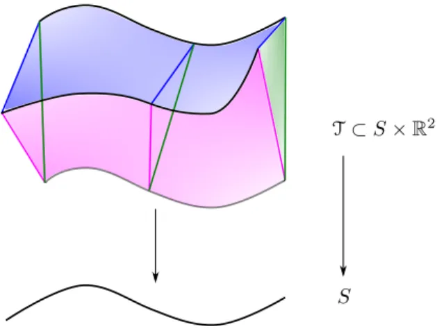
We will now attempt to define moduli functors of labelled and unlabelled triangles. Since we are primarily interested in constructing these moduli spaces as topological spaces, we will consider the category Top of topological spaces and consider representability as a topological space.

Example 0.4.35(Labelled triangles). IfS is a topological space, then we define afamily of labelled triangles overS as a tuple (T, σ1, σ2, σ3) whereT⊂S×R2

is a closed subset andσi:S →T are continuous sections fori = 1,2,3 of the

projection T → S such that for every s ∈ S, the subset Ts ⊂R2 is a labelled

(29)

S

T⊂S×R2

Figure 13: A family of labelled triangles over a curve. Likewise, we define themoduli functor of labelled trianglesas

FM: Top→Sets, S7→ {families (T, σ1, σ2, σ3) of labelled triangles}

We claim this functor is represented by the topological space of full rank 2×3 matrices

M :=

(x1, y1, x2, y2, x3, y3) | det

x2−x1 x3−x1

y2−y1 y3−y1

6

= 0 ⊂R6.

There is a bijection of the setFM(pt) of labelled triangles andM given by taking

the coordinates of the vertices. It is easy to see that this bijection can be promoted to an equivalence of functorsFM

∼

→hM, i.e. to a functorial bijection

FM(S)

∼

→Mor(S, M)

for eachS∈Top, which assigns a family (T, σi) of labelled triangles to the map

S→M wheres7→(σ1(s), σ2(s), σ3(s))∈T.

SinceFM is representable by the topological space M, we have a universal

familyTuniv⊂M ×R2withσ1, σ2, σ3:M →Tuniv. This universal family can be

visualized over the locus (x1, y1) = (0,0) and (x2, y2) = (1,0) by takingFigure 3

and drawing the trianglesaboveeach point rather than ateach point.

Example 0.4.36 (Labelled triangles up to similarity). We say two families (T,(σi)) and (T0,(σi0)) of labelled triangles over S ∈Top aresimilar if for each

s∈S, the labelled trianglesTs andT0sare similar. We define the functor

FMlab: Top→Sets, S7→ {familiesT⊂S×_R2of labelled triangles}/∼

where∼denotes similarity. Recall from (0.2.2) that the assignment of a triangle to its side lengths yields a bijection betweenFMlab and

Mlab=

      

(a, b, c)

a+b+c= 2 0< a < b+c

0< b < a+c

0< c < a+b

       ;

As in the previous example, this extends to an isomorphism of functorsFMlab→

Mor(−, Mlab_{), showing that the topological space}_Mlab _{represents the functor}

(30)

b= 1

a= 1

a+b= 1

-(0,1,1) (1,0,1)

(1,1,0)

Mlab

a c b

(31)

Example 0.4.37 (Unlabelled triangles up to similarity). In Examples 0.4.35

and0.4.36, we considered the moduli functor oflabelledtriangles up to isomorphism and similarity, respectively. We now consider the unlabelled version.

IfS is a topological space, afamily of trianglesis a closed subsetT⊂S×R2

such that for alls∈S, the fiberTs⊂R2is a triangle. We say two families T,T0

overS are similar if the fibersTs andTs0 are similar for alls∈S.

We define the functor

F: Top→Sets, S7→ {familiesT⊂S×R2of triangles}/∼

where∼denotes similarity.

This functor isnotrepresentable as there are non-trivial families of triangles

Tsuch that all fibers are similar triangles (Proposition 0.4.23). For instance, we construct a non-trivial family of triangles overS1 _{by gluing two trivial families}

via a symmetry of an equilateral triangle.

Figure 15: A trivial (left) and non-trivial (right) family of equilateral tri-angles. Image taken from a video produced by Jonathan Wise: see http: //math.colorado.edu/~jonathan.wise/visual/moduli/index.html.

0.5 Illustrating example: Grassmanian

As an illustration of the utility of the functorial approach, we introduce the Grass-manian functor Gr(k, n) over_Z(Definition 0.5.1) and show that it is representable by a projective scheme (Proposition 0.5.7). Since the Grassmanian parameterizes subspaces V of a fixed vector space, this moduli problem does not have non-trivial symmetries, i.e. automorphisms, and thus we do not need the language of groupoids or stacks. This also provides a warmup to the representability and projectivity of Hilbert and Quot schemes (??).

0.5.1 Functorial definition

The points of the Grassmanian Gr(k, n) arek-dimensionalquotientsofn-dimensional space.3 _{But what are families of}_k_{-dimensional quotients over a scheme}_S_{? As} motivated byExample 0.4.30, they should be locally free quotients ofOn

S:

Definition 0.5.1. TheGrassmanian functoris Gr(k, n) : Sch→Sets

S7→

On

S Q

Qis a vector bundle of rankk

/∼

3_{Alternatively, the points could be considered as}_k_-dimensional_subspaces_{but in these notes,} we will follow Grothendieck’s convention of quotients.

(32)

where [On S

q

Q ∼[On

S q0

Q0

if there exists an isomorphism Ψ :Q→∼ Q0 such that

On

S q //

q0 Q Ψ Q0

commutes (i.e. q0= Ψ◦q) or equivalently ker(q) = ker(q0).

Pullbacks are defined in the obvious manner. Observe that if k = 1, then Gr(1, n)∼=Pn−1.

0.5.2 Representability by a scheme

In this subsection, we show that Gr(k, n) is representable by a scheme ( Propo-sition 0.5.4). Our strategy will be to find a Zariski-open cover of Gr(k, n) by representable functors; seeDefinition 0.4.17. Given a subsetI⊂ {1, . . . , n} of size

k, let Gr(k, n)I ⊂Gr(k, n) be the subfunctor where for a schemeS, Gr(k, n)I(S)

is the subset of Gr(k, n)(S) consisting of surjections On S

q

Q such that the composition

OI S

eI

−→On S

q

Q

is an isomorphism, whereeI is the canonical inclusion. When there is no possible

ambiguity, we set GrI := Gr(k, n)I.

Lemma 0.5.2. For eachI⊂ {1, . . . , n}of sizek, the functorGrI is representable by affine spaceAk_Z×(n−k)

Proof. We may assume that I = {1, . . . , k}. We define a map of functors

φ:_Ak×(n−k)_→_Gr

I where over a schemeS, ak×(n−k) matrixf ={fi,j}1≤i≤n

1≤j≤k

of global functions onS is mapped to the quotient



   

1 f1,1 · · · f1,n−k

1 f2,1 · · · f2,n−k

. ._. .._.

1 fk,1 · · · fk,n−k 

   

:On_S →Ok

S. (0.5.1)

The injectivity ofφ(S) :_Ak×(n−k)₍_S₎_→_Gr

I(S) is clear. To see surjectivity,

let [On S

q

−→Q]∈GrI(S) where by definition OIS eI

−→On S

q

Qis an isomorphism. The tautological commutative diagram

On S

q _/_/

(q◦eI)−1◦q

Q

(q◦eI)−1

OI S

shows that [On S

q

Q] = [On S

(q◦eI)−1◦q

OI

S]∈Gr(k, n)(S). Since the composition OI

S eI

−→ On S

(q◦eI)−1

OIS is the identity, the k×n matrix corresponding to (q◦

eI)−1◦q has the same form as (0.5.1) for functionsfi,j∈Γ(S,OS) and therefore

φ(S)({fi,j}) = [On S

q

(33)

Lemma 0.5.3. {GrI}is an open cover ofGr(k, n)whereIranges over all subsets of size k.

Proof. For a fixed subsetI, we first show that GrI ⊂Gr(k, n) is an open subfunctor.

To this end, we consider a schemeSand a morphismS→Gr(k, n) corresponding to a quotientq: On_S →Q. LetCdenote the cokernel of the compositionq◦eI:OIS→

Q. Notice that ifC= 0, then qis an isomorphism. The fiber product

FI //

S

[On S q

Q]

GrI //Gr(k, n)

of functors is representable by the open subschemeU =S\Supp(C) (the reader is encouraged to verify this claim).

To check the surjectivity ofF

IFI →S, lets∈Sbe a point. Sinceκ(s)n q⊗κ(s)

Q⊗κ(s) is a surjection of vector spaces, there is a non-zerok×kminor, given by a subsetI, of thek×nmatrixq⊗κ(s). This implies that [κ(s)n q⊗κ(s)

Q⊗κ(s)]∈

FI(κ(s)).

Lemmas 0.5.2and0.5.3together imply:

Proposition 0.5.4. The functor Gr(k, n)is representable by a scheme.

!

a

Warning 0.5.5. We will abuse notation by denoting both the functor and the scheme as Gr(k, n).

Exercise 0.5.6. Use the valuative criterion of properness to show that Gr(k, n)→

SpecZis proper.

0.5.3 Projectivity of the Grassmanian

We show that the Grassmanian scheme Gr(k, n) is projective (Proposition 0.5.7) by explicitly providing a projective embedding using the functorial approach. The

Pl¨ucker embeddingis the map of functors

P: Gr(k, n)→P(

k ^

On SpecZ)

defined over a schemeS by mapping a rankkquotientOn S

q

Qto the correspond-ing rank 1 quotientVk_On

S→

Vk_Q_{. As both sides are representable by schemes,}

the morphismP corresponds to a morphism of schemes via Yoneda’s lemma.

Proposition 0.5.7. The morphismP: Gr(k, n)→_P(VkOn

Spec_Z)of schemes is a closed immersion. In particular, Gr(k, n)is a projective scheme.

Proof. Let I⊂ {1, . . . , n} be a subset which corresponds to a coordinate xI on

P(VkOnSpecZ). Let P(

Vk_On

(34)

P(VkOnSpec_Z)∼= Gr(1, n k

), then _P(VkOn

Spec_Z)I ∼= Gr(1, nk

){I} (viewing {I} as

the corresponding subset of{1, . . . , n_k} of size 1). Since

Gr(k, n)I PI//

P(VkOnSpecZ)I

Gr(k, n) P //P(VkOnSpecZ)

is a cartesian diagram of functors, it suffices to show thatPI is a closed immersion.

Under the isomorphisms ofLemma 0.5.2,PI corresponds to the map

Ak_Z×(n−k)→A(

n k)−1

Z

assigning a k×(n−k) matrixA ={ai,j} to the element ofA(

n k)−1

Z whoseJth

coordinate, whereJ ⊂ {1, . . . , n} is a subset of lengthk distinct from I, is the

{1, . . . , k} ×J minor of thek×nblock matrix



   

1 a1,1 · · · a1,n−k

1 a2,1 · · · a2,n−k

. ._. .._.

1 ak,1 · · · ak,n−k 

   

(of the same form as (0.5.1)). The coordinatexi,j on Ak_Z×(n−k) is the pull back of

the coordinate corresponding to the subset{1,· · · ,bi,· · · , k, k+j} (seeFigure 16).

This shows that the corresponding ring map is surjective thereby establishing that

PI is a closed immersion.

Figure 16: The minor obtained by removing the ith column and all columns

k+ 1, . . . , nother thank+j is preciselyai,j.

Exercise 0.5.8. For a field K, let Gr(k, n)K be theK-scheme Gr(k, n)×ZK,

andp= [Kn q

Q] be a quotient with kernel K= ker(q). Show that there is a natural bijection of the tangent space

TpGr(k, n)K

∼

→Hom(K, Q).

with the vector space ofK-linear mapsK→Q. Exercise 0.5.9.

(35)

(1) Show that the functor P: Gr(k, n)→_P(VkOn

Spec_Z) is injective on points

and tangent spaces.

Hint: You may want to use the identification of the tangent space ofGr(k, n)

from Exercise 0.5.8. Alternatively you can also show it is a monomorphism.

(2) Use Exercise 0.5.6, part (1)above and a criterion for a closed immersion (c.f.[Har77, Prop. II.7.3]) to provide an alternative proof that Gr(k, n)K is

projective.

0.6 Motivation: why the ´

etale topology?

Why is the Zariski topology not sufficient for our purposes? The short answer is that there are not enough Zariski-open subsets and that ´etale morphisms are an algebro-geometric replacement of analytic open subsets.

0.6.1 What is an ´

etale morphism anyway?

I’m always baffled when a student is intimidated by ´etale morphisms, especially when the student has already mastered the conceptually more difficult notions of say properness and flatness. One reason may be due to the fact that the definition is buried in [Har77, Exercises III.10.3-6] and its importance is not highlighted there.

The geometric picture of ´etaleness that you should have in your head is a covering space. The precise definition of an ´etale morphism is of course more algebraic, and there are in fact many equivalent formulations. This is possibly another point of intimidation for students as it is not at all obvious why the different notions are equivalent, and indeed some of the proofs are quite involved. Nevertheless, if you can take the equivalences on faith, it requires very little effort to not only internalize the concept, but to master its use.

A1 A1

x2 x

Figure 17: Picture of an ´etale double cover of_A1_\₀

For a morphismf:X →Y of schemes of finite type overC, the following are

equivalent characterizations of ´etaleness:

• f is smooth of relative dimension 0 (i.e. f is flat and all fibers are smooth of dimension 0);

• f is flat and unramified (i.e. for ally∈Y(_C), the scheme-theoretic fiberXy

is isomorphic to a disjoint unionF

iSpecCof points); • f is flat and ΩX/Y = 0;

(36)

• for all x∈X(_C), the induced map ObY,f(x) →ObX,x on completions is an

isomorphism; and

• (assuming in addition that X and Y are smooth) for all x∈ X(_C), the induced mapTX,x→TY,f(x) on tangent spaces is an isomorphism.

We say thatf is´etale atx∈X if there is an open neighborhoodU ofxsuch that

f|U is ´etale.

Exercise 0.6.1. Show that f: A1 →A1, x7→x2 is ´etale over A1\0 but is not

´etale at the origin.

Try to show this for as many of the above definitions as you can.

´

Etale and smooth morphisms are discussed in much greater detail and generality inSection A.3.

0.6.2 What can you see in the ´

etale topology?

Working with the ´etale topology is like putting on a better pair of glasses allowing you to see what you couldn’t before. Or perhaps more accurately, it is like getting magnifying lenses for your algebraic geometry glasses allowing you to visualize what you already could using your differential geometry glasses.

Example 0.6.2 (Irreducibility of the node). Consider the plane nodal cubic

C defined by y2 ₌ _x2₍_x₋_{1) in the plane. While there is an analytic open}

neighborhood of the nodep= (0,0) which is reducible, there is no such Zariski-open neighborhood. However, taking a ‘square root’ ofx−1 yields a reducible ´etale neighborhood. More specifically, defineC0= Speck[x, y, t]t/(y2−x3+x2, t2−x+1)

and consider

C0→C, (x, y, t)7→(x, y)

Sincey2−x3+x2= (y−xt)(y+xt), we see thatC0 is reducible.

Introduction to Stacks and Moduli