The Geometry of Moduli Spaces of Maps from Curves

The Geometry of Moduli Spaces of Maps from Curves

Thesis by

Seunghee Ye

In Partial Fulfillment of the Requirements for the degree of

Doctor of Philosophy

CALIFORNIA INSTITUTE OF TECHNOLOGY Pasadena, California

2017

To Yang

© 2017 Seunghee Ye

ACKNOWLEDGEMENTS

First, I would like to thank my avdisor, Tom Graber, for his guidance over the past five years. I have learned a lot under his supervision, and his insights helped me get through numerous obstacles that I encountered in my research. I am very grateful for his help and guidance, without which I could not have completed my research. I would also like to thank Tanvir Ahamed Bhuyain, William Chan, Brian Hwang, Emad Nasrollahpoursamami, and Pablo Solis for helpful discussions and their sup-port. I am also grateful for Craig Sutton for having inspired me to pursue research in mathematics.

ABSTRACT

A class of moduli spaces that has long been the interest of many algebraic geome-ters is the class of moduli spaces parametrizing maps from curves to target spaces. Different such moduli spaces have distinct geometry and also invariants associated to them. In this thesis, we will study the geometry of three such moduli spaces,

f

M_g,n([pt/_C×]),QuotC(n,d), andQ₀,₂(G(n,n),d). By understanding the global ge-ometry of each moduli space, we will produce a stratification, which plays a central role in proving a result about invariants associated to the space.

In Chapter 1, we study gauge Gromov-Witten invariants, which are the Euler char-acteristics of admissible classes onMf_g,n([pt/_C×])_{, the moduli space of maps from} stable curves to [pt/C×]. In [1], Frenkel, Teleman, and Tolland show that while

f

M_{g,nis not finite type, thsese gauge Gromov-Witten invariants are well-defined. By}

using a particular stratification ofMf₀,n_{, we prove that when}g =_0,n_{-pointed gauge} Gromov-Witten invariants can be reconstructed from 3-pointed invariants. This reconstruction theorem provides a concrete way to compute gauge Gromov-Witten invariants, and serves as an alternate proof of well-definedness of the invariants in genus 0 case.

TABLE OF CONTENTS

Acknowledgements . . . iii

Abstract . . . iv

Table of Contents . . . v

List of Illustrations . . . vi

Chapter I: Reconstruction Theorem in Gauge Gromov-Witten Theory . . . 1

1.1 Introduction . . . 1

1.2 Reconstruction in quantum K-theory . . . 2

1.3 Moduli stack of Gieseker bundles . . . 5

1.4 Outline . . . 8

1.5 EmbeddingCe_g,n →Mf_g,n+1 _{. . . . 10}

1.6 Stratification ofZe_g,n =Mf_g,n\Ce_g,n−₁ . . . 15

1.7 Type I curves . . . 16

1.8 Type II curves . . . 22

1.9 Type III curves . . . 29

1.10 Cohomology overZe_g,n _{. . . . 30}

1.11 Towards finiteness of χ(Mf₀,n, α) _{. . . . 33}

1.12 String equation and divisor relations onMf₀,n _{. . . . 41}

1.13 Reduction to boundary loci . . . 46

1.14 Admissible classes onΣi . . . 51

1.15 Proof of the reconstruction theorem . . . 55

1.16 Future directions . . . 57

Chapter II: Generating Series for the Poincare Polynomials of Quot Schemes andQ₀,₂(G(n,n),d) . . . 60

2.1 Introduction . . . 60

2.2 Grothendieck ring of varieties and the Poincare polynomial . . . 61

2.3 Grothendieck Quot schemes . . . 63

2.4 Moduli space of stable quotients . . . 64

2.5 Poincare polynomials of punctual Quot schemes . . . 66

2.6 Generating series for Poincare polynomials ofQuotC(n,d) . . . 71

LIST OF ILLUSTRATIONS

Number Page

1.1 Examples of the correspondenceCg,n → Mg,n+1. . . 10

1.2 Examples of the correspondenceCe_g,n →Mf_g,n+1 . . . 12

1.3 Examples of type I curves . . . 15

1.4 Examples of type II curves . . . 15

1.5 Examples of type III curves . . . 16

1.6 Type I curve lying in the image ofCe_g,n−₁. . . 16

1.7 Modular graphs and curves ofW_i,d1 . . . 17

1.8 Modular graphs and curves ofF_i,d1 . . . 17

1.9 Smoothing the node in the dashed circle . . . 18

1.10 Smoothing the node in the dashed circle . . . 18

1.11 Stratification of Z_i1by Z_i,d1 . . . 19

1.12 Choosing a node on two stable components . . . 23

1.13 Choosing a point on a Gieseker bubble . . . 23

1.14 Choosing a node on a stable component and a bubble . . . 23

1.15 Modular graphs and curves ofW_I,(d2 1,d2) . . . 24

1.16 Modular graphs and curves ofY_I,(d2 1,d2) . . . 24

1.17 Modular graphs and curves ofF_I,(2_d 1,d2) . . . 25

1.18 Type II strata and their closure relations . . . 26

1.19 Closer look atU_I,(2_d 1,d2) . . . 26

1.20 Stratification of Z_I2 . . . 28

C h a p t e r 1

RECONSTRUCTION THEOREM IN GAUGE GROMOV-WITTEN

THEORY

1.1 Introduction

In [9], Lee defines quantum K-invariants, which are K-theoretic push-forwards to SpecC of certain vector bundles on Mg,n(X, β). These quantum K-invariants are shown to satisfy several axioms. Moreover, wheng= 0 andX =Pr, Lee and Pand-haripande prove in [10] that there exist divisor relations in Pic(M0,n(Pr, β))which allow one to reconstruct all quantum K-invariants of M0,n(Pr, β) from quantum K-invariants ofM0,1(Pr, β).

In [1], Frenkel, Teleman, and Tolland consider the compactification of the moduli space of maps from curves to a space with automorphisms. They define the moduli stack of Gieseker bundles on stable curves,Mf_g,n_{, and showed that there exist} well-defined K-theoretic invariants in the case where the target is [pt/C×]. Proving well-definedness of these invariants is difficult because the resulting moduli space is complete but not finite type. Their proof of well-definedness of invariants relies on their description of local charts on the moduli stack. While the use of charts allows them to conclude that the invariants are indeed finite, it does not tell us how the invariants can be computed and does not easily generalize to[X/C×]for arbitrary schemeX.

Instead of using local charts, I describe a stratification of Mf_g,n by locally closed strata. When g = 0, this stratification, along with divisorial relations, allows us to reconstructn-pointed invariants from lower pointed invariants.

Theorem 1.1. n-pointed genus 0 gauge Gromov-Witten invariants can be

recon-structed from 3-pointed invariants.

1.2 Reconstruction in quantum K-theory

In this section, we will define the moduli spaces Mg,n(X, β) and the resulting quantum invariants. We then state the reconstruction theorem for quantum K-invariants wheng = 0. The background onMg,nfollows [2] and the discussion of quantum K-invariants follows [9].

The moduli spacesM_g,n(X, β)

Definition 1.1. [2] Let X be a scheme and let β ∈ H₂(X). Then, a stable map of

classβfrom a prestable curve(C,x₁, . . . ,xn)of genusgwithnmarked points,xi, is a morphism f :C → X satisfying the following conditions.

1. The homological push-forward ofCsatisfies f∗([C])= β.

2. Each irreducible component ofCcontracted by f is stable. In other words, if

E is an irreducible component ofCwhich is contracted by f, then

g(E)+n(E) ≥ ₃,

wheren(E)is the number of nodes and marked points onE.

The moduli space of such maps is denoted byM_g,n(X, β).

It follows from the definition that stable maps have finite automorphisms. Using this fact, Kontsevich prove the following theorem.

Theorem 1.2. [8] Let X be a smooth projective scheme overC, and letβ ∈H2(X).

Then,M_g,n(X, β)is a proper Deligne-Mumford stack.

When X = SpecC, we denote Mg,n(SpecC) = Mg,n. There are two classes of morphisms that arise naturally. The first is the class of forgetful morphisms which forget the k-th marked point and stabilize if necessary. We denote the morphism forgetting thek-th marked point by

f tk :Mg,n+1(X, β) → Mg,n(X, β).

We also have the stabilization morphisms which forget the map f : C → X, and stabilize the prestable curve, C, if necessary. This map is denoted by

Quantum K-invariants

Definition 1.2. [11] Let X be a scheme. The Grothendieck group of locally free

sheaves onXis the quotient of the free abelian group generated by the isomorphism classes of the locally free sheaves on X by the relation Í₍₋

1)iFi = 0, whenever 0→ F0 → F1 → · · ·Fk →0is an exact sequence.

The Grothendieck group of locally free sheaves onX is denotedK(X).

If f : X → Y is a proper morphism, we define the K-theoretic push-forward homomorphism f∗ :K(X) → K(Y)by

f∗([F])=

Õ

(−₁)i[Rif∗F].

The K-theoretic push-forward to SpecCis denoted χ.

Now, we define the quantum K-invariants as the K-theoretic push-forwards of certain K-classes onMg,n.

Definition 1.3. [9] The quantumK-invariants are

hγ₁, . . . , γ_n,Fi= χ(M_g,n(X, β),Ovir ⊗ev∗(γ₁⊗ · · · ⊗γ_n) ⊗st∗F),

whereγ₁, . . . , γn∈ K(X), F ∈K(Mg,n), andOvir is the virtual structure sheaf.

While quantum K-invariants do not satisfy all the axioms of cohomological Gromov-Witten invariants [7], they satisfy seven of them, two of which are the splitting axiom and the string equation.

Proposition 1.1. [9] Letg= g₁+g₂andn=n₁+n₂and let

Φ_:M_g

1,n1+1× Mg2,n2+1→ Mg,n

be the map gluing the last marked point ofM_g

1,n1+1 with the first marked point of M_g

2,n2+1. Then, pulled back quantum K-invariants from Mg,n can be written as a sum of products of quantum K-invariants ofM_g

1,n1+1andMg2,n2+1.

Theorem 1.3 _{(String Equation)}. [9] Let f t : Mg,n+1(X, β) → Mg,n(X, β)be the

morphism forgetting the last marked point. LetL_idenote the cotangent line bundle along thei-th marked point. Then, forg= 0we have

π∗ Ovir n

Ö

i=1

1 1−qiLi

! !

= 1+

n

Õ

i=1

qi

1−qi

!

Ovir n

Ö

i=1

1 1−qiLi

where both sides of the equation are formal series in formal variablesqi. Forg ≥ ₁we have

π∗ Ovir 1

1−qH−1

n−₁

Ö

i=1

1 1−qiLi

!

(1.1)

= Ovir 1

1−qH−1 "

1− H−1+

n−₁

Õ

i=1

qi

1−qi

! _n−1 Ö

i=1

1 1−qiLi

! #

, (1.2)

whereH= R0π_∗ω

C/M is the Hodge bundle.

Note that Theorem 1.3 relates(n+1)-pointed quantum K-invariants notinvolving

L_n+1withn-pointed quantum K-invariants.

Reconstruction of quantum K-invariants

In [10], Lee and Pandharipande prove that two relations hold in Pic(M0,n(Pr, β)). These divisor relations, combined with the axioms of quantum K-invariants, show thatn-pointed quantum K-invariants can be reconstructed from 1-pointed invariants. Let β ∈ H2(Pr). Let β1, β2 ∈ H2(Pr) such that β1 + β2 = β. Partition the set

{₁, . . . ,n} _intoS₁and its complementS2:= S₁c. Then, we denote byDS1,β1|S2,β2 the

divisor inM0,nparametrizing reducible curvesC = C1∪C2 such that the marked pointspj ∈Ci if j ∈Si and the images ofCiareβi fori= 1 and 2. Now, define

Di,β₁|j,βj =

Õ

i∈S1|j∈S2

DS1,β1|S2,β2, and Di,j =

Õ

i∈S1,j∈S2,β1+β2=β

DS1,β1|S2,β2.

Denote by Li the class in Pic(M0,n(Pr, β)) corresponding to the i-th cotangent bundle. Then, we have the following theorem.

Theorem 1.4. [10] Let β ∈ H₂(_Pr) and let L ∈ _Pic(_Pr). Then, the following

relations hold inPic(M0,n(Pr, β)).

1. ev∗_i L =ev∗_j L+ hβ,LiLj−

Õ

β₁+β₂=β

hβ₁,LiDi,β₁|j,β₂.

2. L_i+L_j = Di|j.

With Theorem 1.4, Lee and Pandharipande prove the reconstruction theorem for invariants in both quantum cohomology and quantum K-theory.

1. LetR ⊂ H∗(X)be a self-dual subring generated by Chern classes of elements ofPic(X). Suppose

(τ_i

1(γ1), . . . , τkn−1(γn−1), τkn(ξ))=0

for all n-pointed invariants with γi ∈ R and ξ ∈ R⊥. Then, all n-pointed invariants of classes of Rcan be reconstructed from 1-point invariants ofR.

2. Let R ⊂ K∗(X) be a self-dual subring generated by elements of Pic(X).

Suppose

(τ_i

1(γ1), . . . , τkn−1(γn−1), τkn(ξ))=0

for alln-pointed invariants withγi ∈ Randξ ∈ R⊥. Then, alln-pointed quan-tum K-invariants of classes ofR can be reconstructed from 1-point quantum K-invariants ofR.

1.3 Moduli stack of Gieseker bundles

We will now present the moduli stack of Gieseker bundles as defined in [1]. Moduli stack of Gieseker bundles arise when studying the moduli space of maps from prestable curve to spaces with automorphisms such as [pt/C×]. We recall the definition of families of prestable marked curves.

Definition 1.4. (π _: C → B,{σ_i|i ∈ I}) is called a family of prestable marked

curves over a base schemeBif

1. π : C → B is a flat proper morphism whose fibers are connected curves of

genusgwith at-worst-nodal singularities, and

2. I is an ordered indexing set such that for all i, σi : B → C is a section not

passing through nodes of fibers, and

If all rational components of C has at least 3 special points, we say (C, σ_i) is a family of stable marked curves.

We will always assume that any rational component of a fiber ofπ has at least two special points.

of identifications of the two fibers is isomorphic toC×, the moduli stack of principal

C×-bundles on stable curves fails to be complete.

To make the space complete, we consider all Gieseker bundles on stable curves.

Definition 1.5. [1] Let (C, σ_i) be a stable marked curve. A Gieseker bundle on

(C, σ_i)is a pair(m,L)consisting of

1. a morphismm:(C0, σ_i0) → (C, σi)such thatmis an isomorphism away from preimages of nodes ofC, and the preimages of nodes ofCare either nodes or aP1with two special points; and

2. a line bundleL onC0such that the degree ofL restricted to every unstable P1has degree 1. Such unstable rational components ofC0are called Gieseker bubbles.

Then,Mf_g,n_{is defined to be the moduli stack of Gieseker bundles on stable genus}g_, n-pointed curves.

Definition 1.6. [1] The stackMf_g,nof Gieseker_C×-bundles on stable genusgcurves

withnmarked points is a fibered category whose objects are(X,C, σ_i,P), where

1. X is a test scheme,

2. π _:C → X is a flat projective family of prestable curves with marked points

σi : X →C, and

3. p:P →Cis a Gieseker bundle on the stabilization ofC.

The morphisms in this category are commutative diagrams

P f˜ //

p

P0

p0

C f //

π

C0

π

X

σi

H

H

/

/_X0 σ0

i

V

V

,

f

M_{g,ncarries several universal families. It has a family of stable curves of genus}g

withnmarked pointsπ :Ce_g,n→Mf_g,n_withσ_{i :}Mf_g,n→C_{, and a Gieseker bundle} p:Pg,n → Ceg,n. The universal Gieseker bundle defines a mapϕ :Ceg,n→ [pt/C×]. We define the evaluation maps evi =ϕ◦σi :Mf_g,n → [pt/_C×].

The moduli space, Mf_g,n_{, is a disjoint union of components corresponding to the} total degree of the Gieseker bundle. Each of the components ofMf_g,n _{is complete} but is not finite type in general. For example, consider the component of the moduli space Mf₀,_{4 corresponding to total degree} D_{. There are infinitely many Gieseker} bundles over reducible curve with two components,C =C1∪C2, such that the line bundle, L, has degreesd1 andd2overC1 andC2and d1+d2 = D. Thus,Mfg,nis not finite type and therefore not proper. However, the following properties hold for

f

M_g,n.

Proposition 1.2. [1]

1. Mf_g,nis locally of finite type and locally finitely presented.

2. Mf_g,nis unobstructed.

For a prestable curve with a Gieseker bundle (C, σi,P), we define its topological type to be the pair(γ,d), whereγ is the modular graph ofC and d :V(γ) → Zis the degree map. The topological type of Gieseker bundles allow us to stratifyMf_g,n.

Proposition 1.3. [1]Mf_g,nadmits a topological type stratification by locally closed

and disjoint substacksM_(γ,d) parametrizing all curves with modular graphγ with degreed. Moreover,M_(γ,d)are of finite type and finite presentation.

Moreover, we know which kinds of deformations of curves can occur.

Lemma 1.1. [1] Let(C, σ_i,P)be aC×bundle on a prestable curve having

topolog-ical type(γ,d). Suppose that we are given a deformation(C0, σ_i0,P0) of(C, σ_i,P) over the Spec of a complete discrete valuation ring. The topological type(γ0,d0)of the generic fiber can be any degree labeled modular graph obtained from(γ,d)by finite combinations of the following elementary operations:

2. Resolve a splitting node: join a pair of adjacent vertices v₁ and v₂ into a

single vertexv, having genusgv = gv1+gv2 and degreedv =dv1+dv2. Delete one edge joiningv₁andv₂, and convert the others to self-edges.

Moreover, all such modular graphs occur in some deformation.

OnMf_g,n_{, there are special K-theory classes that we want to consider.}

Definition 1.7. LetV be a finite dimensional representation of_C×. LetL_i = σ∗

iTπ be the relative tangent sheaf to C at σi. Then, we define the following K-theory classes onMf_g,n.

1. The evaluation bundle isev∗_i[V]= σ_i∗ϕ∗V.

2. The descendant bundles are_ev∗_i[V] ⊗ [L⊗ji

i ], where ji ∈Z. 3. The Dolbeault indexIV ofV is the complexRπ∗ϕ∗V.

4. The admissible line bundlesL are L (_detRπ∗ϕ∗C1)

⊗−q_{, whereq ∈} Q>0.

5. An admissible complex is the tensor product of an admissible line bundle with

Dolbeaut index, evaluation, and descendant bundles

α= L ⊗ Ì a

Rπ∗ϕ∗Va

!

⊗ ⊗_iev∗_iWi ⊗ L_ini

_.

Theorem 1.6. [1] Let α be an admissible class. Let F : Mf_g,n → M_g,n be the

forgetful morphism forgetting the bundle and stabilizing the curve. Then, the derived

push-forwardRF∗αis coherent.

1.4 Outline

LetMf₀,n := Mf₀,n([_pt/_C×])_{be the moduli stack of Gieseker stable bundle with the} universal curveπn:Ce₀,n→ Mf₀,n_{. We will denote the universal bundle by} P₀,n_. Let α = det(Rπ∗ϕ∗C1)−q ⊗ ⊗ev

∗

i Cλi ⊗ L

ai

i

First, we show that one can define an open embeddingCe_g,n→Mf_g,n+1_{. If we denote} the complement of the image of Ce_g,n by Ze_g,n+1_{, using the long exact sequence of} local cohomologies, we obtain

χ(Mf_g,n+1, α)= χ(Ce_g,n, α)+ χ

e Z_g,n+1

(α),

provided all the terms above are finite. Now, since Ce_g,n is the universal curve overMf_g,n _{we can compute} χ(Ce_g,n, α) by pushing forward toMf_g,n _{along the map} πn: Ceg,n→ Mf_g,n_.

χ(Ceg,n, α)= χ(Mf_g,n,Rπ_n∗α).

Therefore, we have

χ(Mf_g,n+1, α)= χ(Mf_g,n,Rπ_n∗α)+ χ e Zg,n+1

(α).

Repeating, we conclude that

χ(Mf_g,n, α)=                     

χ(Mf₀,₃,Rπ∗α)+

Õ 4≤k≤n

χ

e

Z₀,k(Rπ∗α) g= 0

χ(Mf₁,₁,Rπ∗α)+

Õ 2≤k≤n

χ

e

Z_1,k(Rπ∗α) g= 1

χ(Mf_g,₀,Rπ∗α)+

Õ 1≤k≤n

χ

e

Zg,k(Rπ∗α) g ≥ 2

,

where π : Mf_g,n d Mf_g,k,k ≤ n is the composition of π` : Ce<sub>g</sub>,` → Mf_g,` for k ≤ ` ≤ n−_1.

We then stratify Ze_g,n by countably many locally closed strata. This stratification will have the property that forg=0, we can compute χ_Ze

0,n

(α)_{recursively as a finite}

sum of products of lower pointed invariants onMf₀,k_{, where}k <n_.

Moreover, the embedding of Ce_g,n → Mf_g,n+1_{will show that for admissible classes,} α, onMf_g,n+1_{that do not involve ev}∗

n+1Cλn+1 andLn+1, the push-forward ofα|Ceg,nto

f

M_{g,nis an admissible class on}Mf_g,n.

A divisor relation similar to the relation proven in Theorem 1.4 then reduce the problem of computing admissible classes onMf₀,n+1to computing those that do not involve ev∗_n+1Cλn+1 andLn+1. Lastly, understanding the structure of the boundary

loci inCe₀,nasAs× (P1)t bundles over products ofMf₀,n0_{, where}n0< n_{, allows us to} compute χ(Mf₀,n+1)_{as a finite sum of} χ(Mf₀,n0)_wheren0< n_.

1.5 EmbeddingCe_g,n →Mf_g,n+1

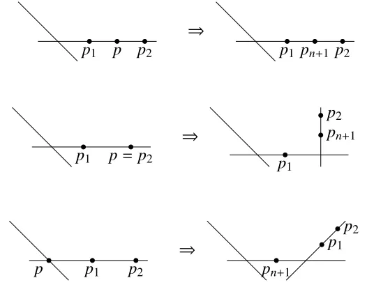
In this section, we will define an embedding Ce_g,n → Mf_g,n+1_{. Recall that we have} a similar embedding for the stable curves. If we letCg,n → Mg,n be the universal curve, we have an embedding Cg,n → Mg,n+1. In short, given a point p on a n -pointed stable curve,(C,p1, . . . ,pn), we can associate to it a(n+1)-pointed curve,

(C0,p0 1, . . . ,p

0

n+1), where

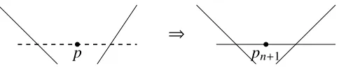
1. if p ∈ C is not a special point, thenC0 = C, p0_i = pi for alli = 1, . . . ,n, and pn+1= p; or

2. if p ∈ C is a special point, then (C0,p0₁, . . . ,p0_n+1) is the stable curve whose stabilization after forgetting p0_n+1isC, with the images ofp0_i under the stabi-lization are pi fori = 1, . . . ,n and pfori = n+1. In other words,C0is the stable curve obtained fromC by adding a rational component atpwith three special points, one of which isp0_n+1.

Figure 1.1 show a few examples of the correspondence described above. In the second and third examples in the figure, the components containingpn+1are rational.

⇒

p₁ p p₂ p₁ pn+1 p₂

⇒

p₁ p= p₂

p₁

p₂ pn+1

⇒

p₁

p p₂ pn+1

p₂ p₁

Figure 1.1: Examples of the correspondenceCg,n → Mg,n+1.

In other words, we consider a resolution of Cg,n ×_M

g,n Cg,n along the subscheme

is a(n+1)-pointed, genusg stable curve. This gives us the desired embedding of

C_g,n→ M_g,n+1.

More precisely, we have the following theorem by Knudsen.

Theorem 1.7. [6] Consider aS-valued point ofC_g,n, i.e. ann-pointed stable curve

π : X → Swithnsections, σ1, . . . , σn, and an extra section∆. Let Ibe the ideal sheaf of∆, and defineK onX by the exact sequence

0 //OX //Iν⊕ OX(σ1+· · ·+σn) //K //0,

where δ : OX → Iν ⊕ OX(σ1+· · ·+ σn) is the diagonal, δ(t) = (t,t). Now, let Xs := Proj(SymK). Then, σ1, . . . , σn,∆have unique liftingsσ

0

1, . . . , σ

0

n+1making

Xs into a(n+1)-pointed stable curve with Xs → X a contraction. Moreover, this

gives rise to an embedding

C_g,n → M_g,n.

We will use a similar strategy to define our embedding of Ce_g,n → Mf_g,n+1_{. Let}

(C,p₁, . . . ,pn,P)be a Gieseker bundle parametrized by a point ofMf_g,n_{and let} p∈ C. Then, we define a Gieseker bundle on a(n+1)-pointed curve,(C0,p0₁, . . . ,p0_n+1,P0) as follows:

1. ifp∈Cis not a special point, thenC0=C,p0_i = pifori =1, . . . ,n,p0_n+1= p, andP0= P; or

2. if p ∈ C is a special point, thenC0 is the curve obtained fromC by adding a rational component at p with three special points, one of which is p0_n+1. The map, ϕ : C0 → C, contracting the component containing p0_n+1 is an isomorphism away from p ∈ C, and the images ofp0_i are pi fori = 1, . . . ,n. Finally, we defineP0:= ϕ∗P.

Note thatP0does satisfy the Gieseker condition. We always have a mapϕ:C0→C which forgets p0_n+1 and stabilizes the component containing p0_n+1 if necessary. In both cases, P0 = ϕ∗P and note that all Gieseker bubbles of C0 are preimages of Gieseker bubbles ofC1. Hence,P0satisfies the Gieseker conditions sincePsatisfies them.

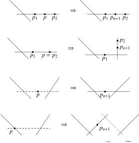
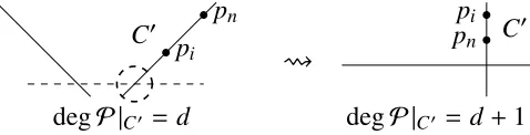
Figure 1.2 shows a few examples of the correspondence described above. The dashed lines in third and fourth figures represent Gieseker bubbles, which are

unstable rational components with two nodes over which the line bundle has degree 1. In the first and third examples, the line bundle over the(n+1)-pointed curve is the same as the line bundle over then-pointed curve as the two curves are the same. In second and fourth examples, p collides with a special point on the n-pointed curve and the corresponding(n+1)-pointed curve has an extra rational component containing pn+1. In these cases, the line bundle over the(n+1)-pointed curve has degree 0 over the component containing pn+1. Over the other components, the line bundle remains “unchanged”.

⇒

p₁ p p₂ p₁ pn+1 p₂

⇒

p₁ p= p_{2 p}

1

p₂ pn+1

⇒

p pn+1

⇒

p pn+1

Figure 1.2: Examples of the correspondenceCeg,n →Mf_g,n+1

In other words, we can define an embedding Ce_g,n → Mf_g,n+1 _{as follows. Let} πn : Ceg,n → Mf_g,n _{be the universal curve over} Mf_g,n_{. Then, we have sections} σi :Mf_g,n→ Ceg,nfori =1, . . . ,n. Let Di := σi∗(Mf_g,n)_{and let}Dsing_{be the locus of} singular points of the fibers ofπn.

Let∆ ⊂ Ce_g,n×

f

Mg,n Ceg,n be the diagonal. Then, by using the analogous sheaf, K,

defined in Theorem 1.7, we get a contraction

ε: Ce:=Proj(SymK) → Ce_g,n×

f

Composing with the projection from the fiber product toCe_g,nwe get ˜

π = pr₂◦ε_:C →e Ce_g,n×

f

Mg,nCeg,n→ Ceg,n,

such that the bundle(pr1◦ε)

∗_P

g,nis a Gieseker bundle overCe_g,n. As in Theorem 1.7, the sections,σi, have unique lifts, giving us nsectionseσi : Ceg,n → Ce. The lift of the diagonal,∆, gives us another section, which we will denote byeσn+1. Therefore,

(Ce,_eσ₁, . . . ,_eσ_n+1,(pr₁◦ε)∗P_g,n)is a family of Gieseker bundles overCe_g,nwith(n+1) sections. Hence, we get a map Ce_g,n → Mf_g,n+1 _{which is an open embedding. We} have the following diagram:

e

C  //

e π=pr2◦ε

% % ε e

C_g,n+1

πn+1

e

C_g,n× f M_g,nCeg,n

pr_{2 //}

pr1

e

C_g,n

πn

 _//

f

M_g,n+1

e

C_g,n πn //Mf_g,n

Note that ϕ∗C1 eev

∗

n+1C1, where ϕ : Ceg,n → [pt/C×] and even+1 : Mfg,n+1 →

[pt/_C×]_.

Now, we consider the restriction toCe_g,nof the determinant bundle and the evaluation bundles onMf_g,n+1_{. In particular, we want to compare these line bundles to the} pull-backs of their analogs fromMf_g,n_.

Proposition 1.4. Let πn : Ceg,n → Mf_g,n be the universal curve, and consider the

embedding of Ceg,n → Mf_g,n+1 described above. Then the following are true over e

C_g,n.

1. For alli = 1, . . . ,n, πn∗◦ev ∗

i Cλ eve

∗

iCλ, whereevi : Mf_g,n → [pt/_C×]and e

evi :Mf_g,n=1→ [pt/_C×]are the respective evaluation morphisms.

2. detRπn+1∗ϕ_e∗C1 π

∗

ndetRπn∗ϕ∗C1, where ϕ : Ce_g,n → [pt/C×] and ϕ_e : e

C_g,n+1→ [pt/_C×].

Proof. First, let’s consider the evaluation line bundles. We know π∗

n◦ev ∗

i Cλ π ∗ n◦σ

∗ i ◦ϕ

∗

Cλ (σi◦πn)∗ϕ∗Cλ.

By definition, ˜σi is the lift of σi. In other words, ˜π ◦σ˜i σi◦πn. Hence, we see that (σi ◦πn)∗ϕ∗Cλ (π˜ ◦σ˜i)∗ϕ∗Cλ σ˜_i∗(π˜∗ ◦ϕ∗Cλ) eve

∗

pull-back of the evaluation line bundles onMf_g,n_{are isomorphic to the evaluation} line bundles onMf_g,n+1_{when restricted to}Ce_g,n.

Since Ce_g,n → Mf_g,n is flat, we know that π_n∗(Rπ_n∗P) Rpr₂∗(pr∗

1P) and hence, π∗

n(detRπn∗P) detRpr2∗(pr

∗

1P). If ˜ϕ : C → [e pt/C

×_]

, then we know that ˜

ϕ∗

C1 pr

∗

1 ◦ε

∗_◦ϕ∗

C1. Since ε : C →e Ce_g,n×

f

Mg,n Ceg,n simply contracts rational

curves, we have that Rε∗O e

C =OCeg,n×Mf_g,_nCeg,n

. Thus, we conclude that detRpr2∗(pr

∗

1ϕ

∗

C1) detR(pr2◦ε)∗((ε◦pr1)

∗_◦ϕ∗

C1) detRπ˜∗(ϕ˜

∗ C1).

Sinceeπis the restriction ofπn+1toC →e Ceg,n, the pull-back of the determinant line bundle is isomorphic to the restriction of the determinant line bundle.

Letαbe an admissible class onMf_g,n+1_{, which is a class of the form} α=(_detRπ_n+1∗ϕ∗C1)

−q_{⊗ ⊗}

iev∗i Cλi ⊗ L

ai

i

_.

We are interested in the push-forward ofα|C_eg,ntoMfg,n. We first recall the projection

formula.

Theorem 1.8 _{(Projection formula)}. [4] Let f : X → Y be a morphism of ringed

spaces. LetFbe anO_X-module and letEbe a locally freeO_Y-module of finite rank. Then, for alli,

Rif∗(F ⊗ f∗E) Rif∗(F) ⊗ E.

By the projection formula and the observations above, we have

Rπ_n∗

α|

e Cg,n

Rπn∗ (detRπn+1∗ϕ

∗

C1)

−q_⊗ n+1

Ì

i=1

ev∗iCλi ⊗ L

ai

i

! !

Rπn∗ π∗_n(detRπn∗ϕ∗C1)

−q_⊗ n

Ì

i=1

π∗ nev

∗

iCλi ⊗ L

ai

i

!

⊗_ev∗_n+

1Cλn+1⊗ L

an+1

n+1

!

(detRπn∗ϕ∗C1)

−q _⊗ n

Ì

i=1

ev∗i Cλi

!

⊗ Rπn∗ ev∗_n+1Cλn+1⊗

n+1

Ì

i=1 Lai

i

!

.

In particular, ifαdoes not involve ev∗_n+1Cλn+1 andL an+1

n+1, we have

Rπn∗

α|

e C_g,n

=(_detRπ_n∗ϕ∗_C1)−q⊗ n

Ì

i=1

ev_i∗Cλi

!

⊗ Rπ_n∗ n

Ì

i=1 Lai

i

1.6 Stratification ofZe_g,n=Mf_g,n\Ce_g,n−₁

Now, we will study the complement of the image of Ce_g,n−₁ in Mf_g,n _{and define a} stratification of the complement by a countably infinite collection of locally closed strata.

Recall that we embedded Ce_g,n−₁ in Mf_g,n _{by considering points of the fibers of} πn−₁ : Ce_g,n−₁ → Mf_g,n−₁ as the last marked point and attaching an extra rational component atpif necessary. In particular, anyn-pointed curve such where pnlies on a component with more than 4 special points is in the image of Ceg,n−₁. Hence, a point in Mf_g,n _{is not in the image of} Ceg,n−₁ only if it parametrizes a Gieseker bundle(C,p1, . . . ,pn,P)such that the component containingpn, call itC

0

, becomes unstable after forgettingpn.

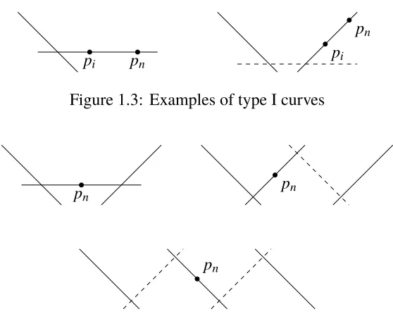
Thus,Cis not in the image ofCe_g,n−₁only ifC0is a rational curve containing precisely three special points2. Since one of the special points is pn, C0can have either one or two nodes. IfC0has exactly one node, we will callCa curve of type I. IfC0has two nodes,C\C0can either have one or two connected components. IfC\C0is the disjoint union of two connected components we will sayC is a curve of type II. If C\C0is connected, we will sayC is of type III.

pi pn pi

pn

Figure 1.3: Examples of type I curves

pn pn

pn

Figure 1.4: Examples of type II curves

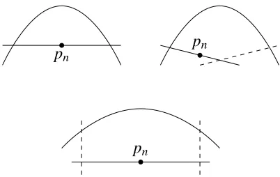
Figures 1.3, 1.4, and 1.5 show examples of type I, II, and III curves, respectively. As before, dashed lines represent Gieseker bubbles over which the line bundle has

2_{This is because all rational components have at least two components and only Gieseker bubbles}

pn

pn

pn

Figure 1.5: Examples of type III curves

degree 1. In all the figures, the component containing pn is rational. All other connected components of the curves in the figures, along with the restriction of the given line bundle, are lower pointed Gieseker bundles3.

Note thatZe_g,n_{is the disjoin union of the strata of type I, II, and III curves. In the} sub-sections that follow, we will stratify subschemes ofZe_g,n_{of type I, II, and III curves.} Also, we will consider the connected component Mf_g,n,D ⊂ Mf_g,n _{parametrizing} Gieseker bundles of some fixed total degreeD.

1.7 Type I curves

Let (C,p1, . . . ,pn,P) ∈ Mf_g,n _{be a type I curve. As before, let} C0 _{denote the} irreducible component of C containing pn. Then, C0 is a rational component containing 2 marked points and a node. Let the marked points be pi andpn. Note that there is only one way a type I curve can be in the image ofCe_g,n−₁. This happens when we choose the point p= pion the fiber as shown in Figure 1.6.

⇒

p= pi

pi

pn C 0

Figure 1.6: Type I curve lying in the image ofCe_g,n−₁

If a type I curve is in the image of Ce_g,n−₁, then the degree of P |_C0 must be 0. Moreover, such curve cannot have a Gieseker bubble attached to C0. Therefore, the type I curves that do not lie in the image of Ce_g,n−₁are the ones such that either degP |C0 _{,0 or}C0_{is attached to a Gieseker bubble.}

3

Fori =1, . . . ,n−1, letZ_i1be the closed subscheme ofMf_g,n_{whose points parametrize} type I curves not in the image ofCe_g,n−₁such thatC0containspnand pi. First, note thatZ_i1is closed inMf_g,n_{: any degeneration of a type I curve is another type I curve;} and the degree ofP |C0 is locally constant away from the Gieseker bubble.

Now, denote by W_i,d1 the locally closed stratum corresponding to the topological types depicted in Figure 1.7, where (γ,D− d) is any topological type of genusg Gieseker bundle of degreeD−d. In other words,W_i,d1 is the stratum corresponding

pi

pn

g=0

d

γ D−d

pi

pn C 0

degP |C0 = d Figure 1.7: Modular graphs and curves ofW_i,d1

to type I curves such that

1. degP |C0 =d_{; and}

2. C0is not attached to a Gieseker bubble. Note thatW_i,d1 ⊂ Ce_g,n−₁if and only ifd =0.

Denote byF_i,d1 the closed stratum corresponding to the topological types depicted in Figure 1.8, where(γ,D−d−1)is any topological type of genusgGieseker bundle of degree D−d −1. In other words, F_i,d1 is the stratum corresponding to type I

pi

pn

g=0

d

g=0 1

γ

D−d−₁ pi

C0 pn

degP |C0 = d Figure 1.8: Modular graphs and curves ofF_i,d1

curves such that

1. degP |C0 =d_{; and}

Note thatF_i,d1 1 Ce_g,n−₁for alliandd.

By Lemma 1.1, we see that for eachiandd, we have W1

i,d =Wi,d1 ∪Fi,d1 ∪Fi,d1−₁.

Moreover, all the curves inZe_g,n_{that are deformations of curves of}F_i,d1 _{are parametrized} by points ofF_i,d1,W_i,d1 andW_i,d1₊₁. More precisely, points ofW_i,d1 parametrize curves obtained from a curve in F_i,d1 by smoothing the node on the connecting Gieseker bubble opposite toC04. Figure 1.9 shows such a deformation.

pi

C0

pn

degP |C0 = d

pi

pn C 0

degP |C0 = d Figure 1.9: Smoothing the node in the dashed circle

Likewise, the points of W_i,d1 ₊₁ parametrize curves obtained from curves in F_i,d1 by smoothing the node onC0as shown in Figure 1.10.

pi

C0

pn

degP |C0 = d

pi

pn C 0

degP |C0 = d+₁ Figure 1.10: Smoothing the node in the dashed circle

We can visualize the stratum of type I curves in the following way:

· · · W1

i,d−1 fF 1

i,d−1 W 1

i,d f Fi,d1 Wi,d1+1 fFi,d1+1 Wi,d1 +2 f· · ·,

where A Bmeans Alies in the closure of B. Now, we define Z_i,d1 as follows.

Z1

i,d =

      

W1

i,d∪Fi,d1 d <0 W1

i,d+1∪Fi,d1 d ≥ 0 .

Keeping in mind W_i,1₀ ⊂ Ce_g,n−₁, we see that Z_i1 = ∪Z_i,d1 gives us the desired stratification ofZ_i1(see Figure 1.11).

4_{We cannot smooth both since such a deformation would result in a curve that lies in the image}

... W1

i,−₂

F1

i,−2 W1

i,−₁

F1

i,−1 W1

i,₀

F1

i,0 W1

i,₁

F1

i,₁

W1

i,−₁

...

⊂ Ce_g,n−₁

Z1

i,−1← Z1

i,₀←

Z1

i,1←

Z1

i,−2←

Figure 1.11: Stratification ofZ_i1by Z_i,d1

Before we move onto type II curves, we give an alternate way of definingZ_i,d1 , which will be useful later. LetU_i,d1 be the stratum of points parametrizing all curves of

e

Z_{g,nobtained by smoothing nodes of curves in}F1

i,d. By Lemma 1.1, this is precisely U1

i,d =Wi,d1 ∪Fi,d1 ∪Wi,d1 +1.

Note that{U_i,d1 | d ∈Z}is an open cover of Z_i1. Then, we can defineZ_i,d1 as follows.

Z1

i,d =

      

U1

i,d\Ui,d1 +1 d < 0 U1

i,d\Ui,d1 −₁ d ≥ 0

.

Geometry ofF1

i,d andZi,d1

We defined F_i,d1 as the stratum of points parametrizing curves of splitting type

({i,n},{i,n}c₎

component, C0, containing pi and pn, and degree e := D−d −1 restricted to the component,C1, containing the other marked points. Hence,

F1

i,d Mfd 0,3×Mf

e

g,n−1,

where we identify the third marked point ofMfd

0,3 and the (n−1)-st marked point ofMfe

g,n−₁as the two nodes on the connecting Gieseker bubble. The marked points

ofMfd

0,3 are denotedpi,pn, and the node p3. The marked points ofMf

e

g,n−1 are the pointspjfor j ,i,n, and the nodepn−1.

Now, we take a closer look at Z_i,d1 . Proposition 4.15 and Corollary 4.16 of [1] tell us that Z_i,d1 is an affine bundle overF_i,d1 .

Proposition 1.5. [1]

1. For d ≥ ₀, Z1

i,d classifies bundles which arise from Fi,d1 by smoothing away the node attachingC0to the connecting Gieseker bubble.

2. For d < 0, Z_i,d1 classifies bundles which arise from F_i,d1 by smoothing away

the node attaching the connecting Gieseker bubble to the components not

containingpn.

3. We have a mapη : Z_i,d1 → F_i,d1 such thatη is the structure map of an affine

bundle.

Note that ourF_i,d1 correspond to those labeled F in [1], and our Z_i,d1 correspond to those labeled Z (when d ≥ 0) andW (when d < 0). 1 and 2 of Proposition 1.5 follow directly from the definition ofZ_i,d1 .

While Frenkel, Teleman, and Tolland do not say exactly which affine bundle η : Z1

i,d → Fi,d1 is, the proof of Proposition 4.15 in [1] contains more information which leads to the following Proposition:

Proposition 1.6. The map η : Z_i,d1 → F_i,d1 from Proposition 1.5 is given by the

bundle

      

(L−1 3 ⊗ P

d

3)(P

e n−1)

−_{1 d ≥}

0

(Pd

3)

−₁

(L−1

n−1⊗ P 3

n−1) d < 0 ,

where

2. L_n−₁is the cotangent bundle along the(n−1)-st section onMfe g,n−₁,

3. Pd

3 is the restriction of the universal bundle along the third section onMf

d

0,3,

and

4. Pe

n−₁is the restriction of the universal bundle along the(n−1)-st section on

f

Me

g,n−₁.

Proof. Letd ≥ 0 and consider curves parametrized by points ofZ_i,d1 . All such curves have splitting type({i,n},{i,n}c). Recall that we denote the component containing pnbyC0, and the other component byC1, where we discard the connecting Gieseker bubble between them if there is one. LetPdenote the universal bundle over curves of Z_i,d1 . Now, we have two trivializations of P restricted to the two components C0 and C1, say t

0

: Ppn → C

×

and t1 : Ppk → C

×

, where k , i,n. These two

trivializations then give us the gluing isomorphism, ι, of the fibers of P over the node. Now, as proof of Proposition 4.15 in [1] points out, scalingt0to 0, we obtain in the limit a connecting Gieseker bubble with a degree 1 transferred from C05. Hence, this gives rise to a mapη : Z_i,d1 → F_i,d1 ford ≥ 0. Similarly, scalingt0to∞ gives a mapZ_i,d1 → F_i,d1 ford <0.

Moreover, the choices of the trivializationst0andt1give us a map between the two fibers of the universal bundles over the nodes onC0andC1, which arePp3andPpn−1,

respectively. As Remark 1.12.1 in [1] explains, this map Ppn−1 → Pp3 is given by

t0/t₁, and is precisely the gluing isomorphism,ι, over the node attachingC0withC1 when we have a type I curve with no connecting Gieseker bubble. When t0 = 0, this mapPpn → Pp3 becomes the 0 map and we get a connecting Gieseker bubble,

as we saw above. Hence, given a section ofη : Z_i,d1 → F_i,d1 , we obtain a morphism

P |_σn−

1 → P |σ3.

Now, since F_i,d1 Mfd

0,3 × Mf

e

g,n−1, we try to write P |σn−1 and P |σ3 in terms of

pull-backs of line bundles over Mfd

0,3 and Mf

e

g,n−1. Let pr1 : F 1

i,d → Mfd 0,3 and pr₂ : F_i,d1 → Mfe

g,n−₁ be the projection maps. First, P |σn−1 is equal to pr ∗

2P

e n−₁

by definition. However, P |σ₃ is not equal to pr₁∗P₃d since P₃d is the restriction of the universal bundle over Mfd

0,3 to σ3 and thus, has 1 lower degree than P |σ3:

degP |σ₃ = d+1. Recall that the mapη: Z_i,d1 → F_i,d1 inserted a connecting Gieseker bubble by scaling the trivialization,t0, to 0 and transferring 1 degree fromC0to the bubble. Hence,P |σ₃ pr₁∗(P₃d⊗ L₃−1).

Therefore, sections ofη: Z_i,d1 → F_i,d1 correspond to sections of

Hompr∗ 2P

e n−1,pr

∗

1(L

−₁

3 ⊗ P

d

3)

pr₁∗(L₃−1⊗ P₃d) ⊗ (pr₂∗Pn−e 1)

−_1.

Hence, we conclude that ford ≥ 0,η: Z_i,d1 → F_i,d1 is the affine bundle given by

(L−1 3 ⊗ P

d

3)(P

e n−1)

−_1.

Ford < 0, the situation is symmetric. Recall that whend < 0, instead of transferring 1 degree to the bubble fromC0, we transfer it fromC1. The mapη : Zi,d1 → Fi,d1 is then defined by scaling the trivialization,t0, to∞. By the same argument as in the d ≥ _{0, case we conclude that}η_: Z1

i,d → Fi,d1 is the affine bundle given by

(Pd

3)

−₁

(L−1

n−1⊗ P

e n−1).

Another way to show thatZ_i,d1 is the affine bundle given by(L−₃1⊗ P₃d)(P_ne−₁) −₁

is by considering the formal neighborhood ofF_i,d1 . Z_i,d1 corresponds to smoothings of the node attachingC0to the connecting Gieseker bubble, which is the marked point p₃onMfd

0,3. Smoothing a node is represented by the formal neighborhood given by T₊⊗T−whereT±denote the tangent bundles at the node on the two components. In our case, those bundles areL₃−1 fromC0, and P₃d (P_n−e ₁)−1 from the connecting Gieseker bubble. The tangent bundle at the node on the connecting Gieseker bubble is P₃d(P_ne−₁)

−₁

since O(1)of the Gieseker bubble is glued on the two nodes, p3 and pn−1, to the fibers Pp3 and Ppn−1. Hence, Z

1

i,d corresponds to the affine bundle overF_i,d1 given by

pr₁∗L−1 3 ⊗

Pd

3 (P

e n−1)

−₁

(L₃−1⊗ P₃d)(Pn−e 1)

−_1.

1.8 Type II curves

Now, we stratify the stratum of type II curves.

Let (C,p1, . . . ,pn,P) ∈ Mfg,n be a type II curve and letC

0

denote the irreducible component ofC containing pn. SinceC is a type II curve,C0contains the marked pointpnand two nodes, andC\C0has two connected components. Note that there are precisely three ways for a type II curve to lie in the image ofCe_g,n−₁.

2. we choose a point on a Gieseker bubble asp(Figure 1.13); or

3. we choose the node on a stable component and a Gieseker bubble asp (Fig-ure 1.14).

⇒

p pn+1

Figure 1.12: Choosing a node on two stable components

⇒

p pn+1

Figure 1.13: Choosing a point on a Gieseker bubble

⇒

p pn+1

Figure 1.14: Choosing a node on a stable component and a bubble

Therefore, a type II curve is in the image ofCe_g,n−₁if and only if either

1. degP |C0 =_{1 and}C0_{is not connected to a Gieseker bubble; or} 2. degP |C0 =_{0 and}C0_{is connected to 0 or 1 Gieseker bubbles.}

For a type II curve, C\C0 has two connected components. For I ⊂ [n− 1] :=

{₁, . . . ,n− ₁} _{such that} |I|,|Ic| ≥ _{2, let} Z2

I be the closed subscheme of Mfg,n

whose points parametrize type II curves not in the image ofCe_g,n−₁such that points

{pi | i ∈ I} and {pi | i < I} are on separate connected components of C\C0. Without loss of generality, denote byC1the curve containing points with indices in I, andC2the other connected component.

that type II curves can have 0, 1, or 2 Gieseker bubbles attached toC0. We will call these strataW2,Y2, andF2, respectively.

Let d1,d2 ∈ Z. We denote by WI,(2d1,d2) the locally closed stratum corresponding

to the topological type depicted in Figure 1.15, where (γi,di) is any topological type of genusgi Gieseker bundle of degree di with marked points ofCi, such that

g =g₁+g₂.

pn γ₁

d₁ g=0_d

γ₂ d₂

d = D−d₁−d₂

pn

Figure 1.15: Modular graphs and curves ofW_I,(d2

1,d2)

In other words,W_I,(2_d

1,d2)is the stratum corresponding to type II curves such that

1. degP |Ci =di; and

2. C0is not connected to any Gieseker bubbles.

We will denote by

W2

I,d :=

Ø

D−d₁−d₂=d

W2

I,(d₁,d₂).

Note thatW_I,d2 ⊂ Ce_g,n−₁if and only ifd =0 or 1 by the discussion from the beginning of the section.

The type II curves with a Gieseker bubble connectingC0withC1will be denoted Y2

I,(d₁,d₂). The topological type of such curves is shown in Figure 1.16.

pn γ₁

d1

g=0 1

g=0

d

γ₂ d2

d = D−d₁−d₂−₁

pn

Figure 1.16: Modular graphs and curves ofY_I,(2_d

1,d2)

We also define

Y2

I,d :=

Ø

D−d₁−d₂=d

Y2

I,(d₁,d₂)∪YI2c_,(d

2,d1)

Note thatY_I,d2 ⊂ Ce_g,n−₁if and onlyd =1. Lastly, we denote byF_I,(2_d

1,d2)the stratum of type II curves with two Gieseker bubbles

with the topological type shown in Figure 1.17. pn γ₁ d1 g=0 1 g=0 d g=0 1 γ₂ d2

d = D−d₁−d₂−₂

pn

Figure 1.17: Modular graphs and curves ofF_I,(2_d

1,d2)

Also, define

F2

I,d :=

Ø

D−d1−d2=d

F2

I,(d1,d2).

Again by Lemma 1.1, we see thatF_I,d2 andF_I,(d2

1,d2)are closed in

f

M_{g,n. Similarly to}

the type I case, letU_I,(2_d

1,d2) denote the stratum of points parametrizing all curves of

e

Z_{g,nthat are obtained by smoothing 0 or 1 of the nodes on each Gieseker bubble of}

curves ofF_I,(2_d

1,d2) 6.

U2

I,(d1,d2) := F

2

I,(d1,d2) ∪Y2

I,(d1,d2) ∪Y2

I,(d1,d2+1) ∪Y2

Ic_,(d

2,d1) ∪Y2

Ic_,(d

2,d1+1) ∪W2

I,(d₁,d₂)∪WI,(d2 ₁+1,d₂)∪WI,(d2 ₁,d₂+1)∪WI,(d2 ₁+1,d₂+1).

Note that{U_I,(d2

1,d2)

| D−d₁−d₂= d} _{forms an open cover of}Z2

I,dinZe_g,n_. Also, the stratum of all smoothings of curves ofF_I,d2 is

U2

I,d =

Ø

D−d1−d2=d

U2

I,(d1,d2)

= F2

I,d∪YI,d2 ∪YI,d2 −₁∪WI,d2 ∪WI,d2 −₁∪WI,d2 −₂.

Note that{U_I,d2 | d ∈Z}forms an open cover ofZ_I2.

We can visualize the closure relations of these type II strata using the following infinite two dimensional grid7in Figure 1.188.

Figure 1.19 showsU_I,(2_d

1,d2) as deformations of curves in

F2

I,(d1,d2). The dashed lines

attached to the nodes on the Gieseker bubbles indicate which deformation happen as we smooth the chosen node.

6

As we saw in Section 1.7, we cannot smooth both nodes of the same Gieseker bubble since such deformation would result in a curve lying in the image ofCeg,n−₁.

7_{The two dimensions correspond to smoothings of the two connecting Gieseker bubbles. The}

W2

I,(d₁−₁,d₂−₁) YI,(d2 ₁−₁,d₂−₁) WI,(d2 ₁,d₂−₁) YI,(d2 ₁,d₂−₁) WI,(d2 ₁+1,d₂−₁)

Y2

Ic_,(d

2−1,d1−1)

F2

I,(d₁−₁,d₂−₁) YI2c_,(d

2−1,d1)

F2

I,(d₁,d₂−₁) YI2c_,(d

2−1,d1+1)

W2

I,(d₁−₁,d₂) YI,(d2 ₁−₁,d₂) WI,(d2 ₁,d₂) YI,(d2 ₁,d₂) WI,(d2 ₁+1,d₂)

Y2

I,(d₁−₁,d₂) FI,(d2 ₁−₁,d₂) YI2c_,(d

2,d1)

F2

I,(d₁,d₂) YI2c_,(d

2,d1+1)

W2

I,(d₁−₁,d₂+1) YI,(d2 ₁−₁,d₂+1) WI,(d2 ₁,d₂+1) YI,(d2 ₁,d₂+1) WI,(d2 ₁+1,d₂+1)

U2

I,(d₁−₁,d₂−₁)

U2

I,(d1,d2)

Figure 1.18: Type II strata and their closure relations

(d₁,d₂+1) (d1+1,d2+1)

(d₁,d₂+1) (d1+1,d2+1)

Figure 1.19: Closer look atU_I,(2_d

We are finally ready to define our stratification ofZ2_I. Define

Z2

I,d :=

      

U2

I,d\UI,d2 +1 d ≤ 1 U2

I,d\UI,d−2 1 d ≥ 2 .

We also define

Z2

I,(d₁,d₂) := ZI,d2 ∩UI,(d1,d2).

Recalling thatW_I,2₀,W_I,2₁,Y_I,2₁ ⊂ Ce_g,n−₁, we see that Z_I,d2 stratify Z_I2. Moreover, for eachd, Z_I,d2 is the disjoint union

Z2

I,d =

Ø

D−d1−d2=d

Z2

I,(d1,d2).

Figure 1.20 shows the stratification ofZ_I2by Z_I,d2 andZ_I,(d2

1,d2). All superscripts and

subscripts except for the degrees are suppressed for the sake of simplicity.

In Figure 1.20, d1,d2 ∈ Zare such that D− d1−d2 = 1. The strata that lie in the blue shaded region are the ones that are in the image ofCeg,n−1. The red boxes are theZ2_I,(d0_,d00₎, where(d

0_,

d00)_{are the degrees corresponding to the}F(d0_,d00_{)in the same} box. For example, the box labeled (2.2) correspond to Z_I,(2_d

1,d2−1). Moreover, each

box labeled(d,k)lie in Z_I,d2 . For example, boxes (1.1), (1.2), and (1.3), which are Z2

I,(d₁−₁,d₂+1),Z2I,(d₁,d₂),ZI,(d2 ₁+1,d₂−₁), respectively, all lie inZI,2₁. Note that

D− (d₁−₁) − (d₂+1)= D−d1−d2= D− (d1+1) − (d2−1)=1.

Geometry ofF2

I,(d1,d2)

andZ2

I,(d1,d2)

By the same argument as in the type I case, F2

I,d₁,d₂ Mfd1

g₁,|I|+1×Mf d

0,3×Mf

d2

g₂,|Ic_|+1,

whered = D−d1− d2−2. Also, by Proposition 1.5, we know that there exists a mapη : Z_I,(2_d

1,d2) → F2

I,(d1,d2), which is the structure map of an affine bundle. From

our description ofZ_I,(2_d

1,d2), we know that

1. ford ≥ 2, Z_I,(2_d

1,d2)classifies bundles which arise from F

2

I,(d1,d2)by smoothing

away nodes attaching the connecting Gieseker bubbles toC1andC2; and 2. ford ≤ 1, Z_I,(d2

1,d2)classifies bundles which arise from F

2

I,(d₁,d₂)by smoothing

Wd₁−₁,d₂−₂ Yd₁−₁,d₂−₂ Wd₁,d₂−₂ Yd₁,d₂−₂ Wd₁+1,d₂−₂ Yd₁+1,d₂−₂ Wd₁+2,d₂−₂

Yd₁−₁,d₂−₂ Fd₁−₁,d₂−₂ Yd₁,d₂−₂ Fd₁,d₂−₂ Yd₁+1,d₂−₂ Fd₁+1,d₂−₂ Yd₁+2,d₂−₂

Wd1−1,d2−1 Yd1−1,d2−1 Wd1,d2−1 Yd1,d2−1 Wd1+1,d2−1 Yd1+1,d2−1 Wd1+2,d2−1

Yd1−1,d2−1 Fd1−1,d2−1 Yd1,d2−1 Fd1,d2−1 Yd1+1,d2−1 Fd1+1,d2−1 Yd1+2,d2−1

Wd1−1,d2 Yd1−1,d2 Wd1,d2 Yd1,d2 Wd1+1,d2 Yd1+1,d2 Wd1+2,d2

Yd₁−₁,d₂ Fd₁−₁,d₂ Yd₁,d₂ Fd₁,d₂ Yd₁+1,d₂ Fd₁+1,d₂ Yd₁+2,d₂

Wd1−1,d2+1 Yd1−1,d2+1 Wd1,d2+1 Yd1,d2+1 Wd1+1,d2+1 Yd1+1,d2+1 Wd1+2,d2+1

Yd1−1,d2+1 Fd1−1,d2+1 Yd1,d2+1 Fd1,d2+1 Yd1+1,d2+1 Fd1+1,d2+1 Yd1+2,d2+1

Wd1−1,d2+2 Yd1−1,d2+2 Wd1,d2+2 Yd1,d2+2 Wd1+1,d2+2 Yd1+1,d2+2 Wd1+2,d2+2

4.1 3.2 2.3

3.1 2.2

2.1

1.1 0.1 -1.1

1.2 0.2

1.3

Figure 1.20: Stratification ofZ_I2

Figure 1.21: Z2_I,(d

1,d2)when

D−d₁−d₂ ≥ ₂

Proposition 1.7. The mapη: Z_I,(d2

1,d2) → F2

I,(d₁,d₂)is the structure map of the affine bundle         

L−1

|I|+1⊗ P

d1 |I|+1

(Pd 1) −₁ O e M₂

⊕ O e

M₁(P₃d) −₁

L−1

|Ic_|+1⊗ P

d2

|Ic_|+1 d ≥ 2

Pd1 |I|+1

−1

L−1 1 ⊗ P

d 1 O e M2 ⊕ O e M2

L−1 3 ⊗ P

d

3

Pd2 |Ic_|+1

−1

d ≤ ₁, where

1. L_|I|+1is the cotangent bundle along the(|I|+₁)-st section,σ|I|+1, onMfd1 g₁,|I|+1;

2. Pd1

|I|+1is the restriction toσ|I|+1of the universal bundle overMf d₁

g1,|I|+1 ;

3. L₁andL₃are the cotangent bundles alongσ₁andσ₃onMfd 0,3;

4. Pd

1 and P

d

3 are the restrictions to σ1 and σ3 of the universal bundle over f

Md

0,3;

5. L_|Ic_|+1is the cotangent bundle alongσ_|Ic_|+1onMfd2

g₂,|Ic_|+1; and

6. Pd2

|Ic_|+1is the restriction toσ|Ic_|+1of the universal bundle overMfd2 g2,|Ic|+1

.

1.9 Type III curves

A necessary and sufficient condition for a type III curve to be in the image ofCe_g,n−₁ is the same as the condition for type II curves. Denote by Z3the closed subscheme of Mf_g,n _{whose points parametrize type III curves that do not lie in the image of}

e

C_{g,n−1. For} j ∈ _{Zconsider the strata} F3

d whose points parametrize type III curves

such that

1. degP |C0 = j_{; and}

2. C0is connected to two Gieseker bubbles.

Then, for j ≥ 0, we defineZ3_j recursively as Z3

j =

U3

j ∩Z3

\ Ø

0≤k≤j−1 Z3

k,

Similarly for j ≤ −1, we defineZ3_j recursively as Z3

j =

U3

j ∩Z3

\ Ø

j+1≤k≤−₁

Z3

k.

By the same argument we see that Z3_j is locally closed for all j ∈Zand that χ_Z3(F)= Õ

j∈Z

χ_Z3

j

(F).

For j ≥0, Z3_j parametrize all type III curves that are obtained from curves ofF_j3by smoothing the nodes onC0. For j ≤ −1, Z3_j parametrize all type III curves that are obtained from curves ofF_j3by smoothing the nodes on the two connecting Gieseker bubbles that do not lie onC0.

1.10 Cohomology overZe_g,n

Recall that we would like to compute χ(Mf_g,n, α)_{, where}α_{is an admissible bundle} on Mf_g,n_{. In order to compute} χ(Mf_g,n, α)_{, we use the stratification of} Mf_g,n _{as a} union of Ce_g,n, Z_i1, Z_I2, and Z3. First, we recall the definition of cohomology with support on a locally closed subscheme.

Definition 1.8. [5] LetX be a topological space and let Z ⊂ X be a locally closed

subset. Define the sections ofFwith support inZ as

Γ_Z(X,F):= {s ∈ F(X) | Supp(s) ⊂ Z}.

Then,Γ_Z is left exact but not necessarily exact. We define the right derived functors ofΓ_Z to be the local cohomology groups with support withZ,

H_Zi(X,F):= RiΓZ(X,F).

Local cohomologies satisfy several properties.

Proposition 1.8. [5] Let Z be a locally closed subset of X. Suppose Z ⊂ Y ⊂ X.

Then,

Hi_Z(X,F)= H_Zi(Y,F|_Y), for alliand for all sheavesFon X.

Proposition 1.9. LetZ ⊂ X be an open subset. Then,

Hi_Z(F)= Hi(Z,F),

for alliand for all sheavesFon X.

When Z ⊂ X is a locally closed subset, there is an associated long exact sequence of cohomologies.

Lemma 1.2. [5] Let X be a topological space and let Z ⊂ X be a locally closed

subset. LetZ0⊂ Z be closed inZ and letZ00 := Z\Z0. Then, we have the following long exact sequence of local cohomologies for any abelian sheafFon X:

0→H0_Z0(F) →H_Z0(F) →H_Z000(F) →H_Z10(F) →H_Z1(F) →H_Z100(F) → · · · .

Corollary 1.1. Let X be a topological space and let Z ⊂ X be a locally closed

subset. LetY = X \Z and letFbe a sheaf on X. Then, we have the following long exact sequence of local cohomologies:

0→ H_Z0(F) →H0(X,F) →H0(Y,F) → H_Z1(F) →H1(X,F) →H1(Y,F) → · · · .

Proof. The long exact sequence is the one associated to the triple Z,Y ⊂ X from Lemma 1.2, where the local cohomologies with support on open subsets of X are replaced with regular cohomologies using Proposition 1.9. Note thatCeg,n−₁is open inMf_g,n_{and thus,}Ze_g,n_{is closed. By Corollary 1.1, for any} sheafFonMf_g,n, we have the following long exact sequence of local cohomologies 0→ H0

e Z_g,n

(F) →H0_{(F) →H}0₍ e

C_g,n−1,F) →H1

e Zg,n

(F) →H1_{(F) →H}1₍ e

C_g,n−1,F) → · · · ,

whereHi(F):= Hi(Mf_g,n,F). Hence, if all the following terms are well-defined, we have

χ(Mf_g,n,F)= χ(Ce_g,n−₁,F)+ χ

e Zg,n(F).

In following sections, we will show that when g = 0, the terms are indeed well-defined and that the equation above gives us a formula for computing n-pointed invariants, χ(Mf₀,n, α), from lower pointed invariants, χ(Mf₀,m, α), wherem< n. Note that the strataZ1,Z2, andZ3are a pairwise disjoint collection of locally closed strata. Hence, by using Lemma 1.2 onZ1,Z2,Z3 ⊂ Ze_g,n, we get

χ

e