Sample Size Planning for the Squared Multiple Correlation Coefficient: Accuracy in Parameter Estimation via Narrow Confidence Intervals

(1)

ISSN: 0027-3171 print/1532-7906 online DOI: 10.1080/00273170802490632

Sample Size Planning for the Squared

Multiple Correlation Coefficient:

Accuracy in Parameter Estimation

via Narrow Confidence Intervals

Ken Kelley

Department of Management

University of Notre Dame

Methods of sample size planning are developed from the accuracy in parameter approach in the multiple regression context in order to obtain a sufficiently narrow confidence interval for the population squared multiple correlation coefficient when regressors are random. Approximate and exact methods are developed that provide necessary sample size so that the expected width of the confidence interval will be sufficiently narrow. Modifications of these methods are then developed so that necessary sample size will lead to sufficiently narrow confidence intervals with no less than some desired degree of assurance. Computer routines have been developed and are included within the MBESS R package so that the methods discussed in the article can be implemented. The methods and computer routines are demonstrated using an empirical example linking innovation in the health services industry with previous innovation, personality factors, and group climate characteristics.

In the behavioral, educational, managerial, and social (BEMS) sciences, one of the most commonly used statistical methods is multiple regression. When designing studies that will use multiple regression, sample size planning is often considered by researchers before the start of a study in order to ensure there Correspondence concerning this article should be addressed to Ken Kelley, Department of Management, Mendoza College of Business, University of Notre Dame, Notre Dame, IN 46556. E-mail: [email protected]

524

(2)

is adequate statistical power to reject the null hypothesis that the population squared multiple correlation coefficient (denoted with an uppercase rho squared, P2) equals zero. Planning sample size from this perspective is well known in the sample size planning literature (e.g., Cohen, 1988; Dunlap, Xin, & Myers, 2004; Gatsonis & Sampson, 1989; Green, 1991; Mendoza & Stafford, 2001). However, with the exception of Algina and Olejnik (2000), sample size planning when interest concerns obtaining accurate estimates of P2 has largely been ignored. With the emphasis that is now being placed on confidence intervals for effect sizes in the literature, and with the desire to avoid “embarrassingly large” confidence intervals (Cohen, 1994, p. 1002), planning sample sizes so that one can achieve narrow confidence intervals continues to increase in importance. Planning sample size when one is interested in P2 _{can thus proceed in (at least)}

two fundamentally different ways: (a) one that plans an appropriate sample size based on some desired degree of statistical power for rejecting the null hypothesis that P2_D₀_{(or some other specified value) and (b) one that plans an appropriate}

sample size in order for the confidence interval for P2 _{to be sufficiently narrow.}

The purpose of this article is to provide an alternative to the power analytic approach to sample size planning for the squared multiple correlation coefficient in theaccuracy in parameter estimation(AIPE) context (Kelley, 2007c; Kelley & Maxwell, 2003, 2008; Kelley, Maxwell, & Rausch, 2003; Kelley & Rausch, 2006; Maxwell, Kelley, & Rausch, 2008). The general idea of the AIPE approach to sample size planning is to obtain a confidence interval that is sufficiently narrow at some specified level of coverage and thus avoid wide confidence intervals, which illustrate the uncertainty with which the parameter has been estimated. The theoretical differences between the AIPE and power analytic approaches to sample size planning and the implications for the cumulative knowledge of an area are delineated in Maxwell et al. (2008).1

As recommended by Wilkinson and the American Psychological Association (APA) Task Force on Statistical Inference (1999), researchers should “always present effect sizes for primary outcomes” (p. 599). Similarly, the American Educational Research Association recently adopted reporting standards that state, “An index of the quantitative relation between variables” (i.e., an effect size) and “an indication of the uncertainty of that index of effect” (i.e., a confidence interval) should be included when reporting statistical results (2006, p. 10). Although not true for effect sizes in general, BEMS researchers have tended to report the estimated squared multiple correlation coefficient. However, Wilkinson and the APA Task Force go on to recommended that “interval estimates should

1_{The use of the term “accuracy” in this context is the same as that used by Neyman (1937)} in his seminal work on the theory of confidence interval construction: “The accuracy of estimation corresponding to a fixed value of1!’may be measured by the length of the confidence interval” (p. 358; notation changed to reflect current usage).

(3)

be given for any effect sizes involving principal outcomes” (1999, p. 599), something that has not historically been done. This is not a problem unique to BEMS research: it seems confidence intervals for P2 have not historically been reported in any domain of research. Nevertheless, with increased emphasis on confidence intervals for effect sizes, there is almost certainly going to be an increase in the use of confidence intervals for P2. Indeed, confidence intervals for effect sizes may well be the future of quantitative research in the BEMS sciences (Thompson, 2002).

One problem waiting to manifest itself when researchers routinely begin to report confidence intervals for P2 is that, even with sufficient statistical power, the widths of the confidence interval for P2 might be large, illustrating the uncertainty with which information is known about P2_{. This article fills a void}

in the multiple regression and sample size planning literatures by developing methods so that sample size can be planned when there is an interest in achieving a narrow confidence interval for P2_{. The first method developed yields necessary}

sample size so that theexpected width of the obtained confidence interval for P2 is sufficiently narrow. For example, a researcher may plan sample size so that the expected width of the confidence interval for P2 is .10. Because the confidence interval width is itself a random variable based in part onR2, the usual (although biased) estimate of P2, the observed width is not guaranteed to be sufficiently narrow even though its expected width is sufficiently narrow. A modified approach yields the necessary sample size so that the confidence interval for P2will be sufficiently narrow with some desired degree of assurance, where the assurance is a probabilistic statement. For example, a researcher may plan sample size so that the confidence interval for P2 is no wider than .10 with 99% assurance.

Multiple regression is used with fixed and/or random regressors. Distribu-tional characteristics of regression coefficients are different for fixed and random regressors due to the increased randomness in the model when regressors are random because of the sample-to-sample variability (e.g., Gatsonis & Sampson, 1989; Rencher, 2000; Sampson, 1974).2 _{The sample size procedures developed} here are for the case where regressors are random, which is how multiple regression is generally used in the BEMS sciences. Confidence intervals for P2 have not often been considered in applied work (but see Algina & Olejnik, 2000; Ding, 1996; Kelley & Maxwell, 2008; Lee, 1971; Mendoza & Stafford, 2001; Smithson, 2001; and Steiger & Fouladi, 1992, for discussions and pro-cedures of confidence interval formation for P2). However, with the strong

2_{The term “regressors” is used as a generic term to denote the}_{K X}_{variables. In other contexts} the regressors are termed independent, explanatory, predictor, or concomitant variables. The term “criterion” is used as a generic term for the variable that is modeled as a function of theKregressors. In other contexts, the criterion variable is termed dependent, outcome, or predicted variable.

(4)

encouragement from methodologists and important professional associations, as well as the development and recognition of software to implement confidence intervals for P2, there is likely to be an increase in reporting confidence intervals for P2.

The article begins with a discussion of confidence interval formation for P2 and idiosyncratic estimation issues that become important when the sample size procedures are developed. Development of sample size planning for AIPE in the context of P2 is then given. Results of a Monte Carlo simulation study are summarized that illustrate the effectiveness of the proposed procedures. The procedures used and methods developed in this article can be easily implemented in the program R (R Development Core Team, 2008) with the MBESS package (Kelley, 2007a, 2007b, 2008; Kelley, Lai, & Wu, 2008). A demonstration of the methods developed is given using an empirical example, where the methods are implemented with MBESS in the context of innovation in the health services industry linking innovation with previous innovation, personality factors, and group climate characteristics (Bunce & West, 1995). Because the value of P2_{is of}

interest in many applications of multiple regression, not literally the dichotomous reject or fail to reject decision of a null hypothesis significance test, it is hoped that researchers will consider the AIPE approach instead of or in addition to the power analytic approach when planning a study where multiple regression will be used to analyze data.

ESTIMATION AND CONFIDENCE INTERVAL FORMATION FOR P2

The common estimate of P2_,_R2_{, is positively biased and thus tends to}

overes-timate the degree of linear relationship between theK regressor variables and the criterion variable in the population, especially when sample size,N, is very small. The expected value ofR2 _{given P}2_,_N_{, and}_K _{is given as}

E! R2j" P2; N; p#$ D1!N !K!1 N !1 .1!P 2_/_H % 1I1IN C1 2 IP 2 & (1) for multivariate normal data, where H is the hypergeometric function (Johnson, Kotz, & Balakrishnan, 1995, p. 621; Stuart, Ord, & Arnold, 1999, section 28.32). For notational ease, E!

R2_j"

P2; N; p#$

will be written as EŒR2_!_.

As discussed by Steiger (2004), “confidence intervals for the squared multiple correlation are very informative yet are not discussed in standard texts, because a single simple formula for the direct calculation of such an interval cannot be obtained in a manner that is analogous to the way one obtains a confidence interval for the population mean” (p. 167). The difficulties when forming a

(5)

confidence interval for P2 arise for several reasons. First, there is no closed form solution for confidence intervals for P2. The lack of closed form solutions requires iterative algorithms for forming the confidence intervals. Second, there is a nontrivial difference in the distribution of R2 when regressors are fixed compared with when they are random when P2 > 0. Fixed regressors are specified a priori as part of the design of the study. These values are “fixed” in the sense that over theoretical replications of the study, the values of the regressors would not change. This is contrasted to the situation of random regressors, where the regressors are a function of the particular sample. These values are “random” in the sense that over theoretical replications of the study, each sample would yield a different set of regressors. This article focuses only on the case of random regressors, as applications of multiple regression in the BEMS sciences tend to be random. Although confidence intervals for fixed regressor variables are fairly straightforward given the appropriate noncentral

F-distribution routines, confidence interval formation is much more difficult when regressors are random.

Sampson (1974) and Gatsonis and Sampson (1989) provide a discussion of the differences between the fixed and the random regressor models for multi-ple regression. Lee (1971) and Ding (1996) provide algorithms for computing various aspects of the distribution ofR2 for random regressors, which can be used in order to compute confidence intervals. Although the programming of the algorithms underlying the computer programs is not trivial, nearly exact confidence intervals for P2 under the case of random regressors variables can be found with the use of freely available software (e.g., MBESS; Kelley, 2008; MultipleR2; Mendoza & Stafford, 2001; R2; Steiger & Fouladi, 1992) and in other programs indirectly with proper programming (e.g., in SAS; Algina & Olejnik, 2000).

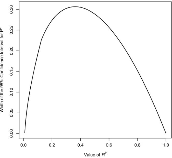
Unlike many effect sizes, there is not a monotonic relation between the width of the confidence interval for P2 _{and the value of}_R2_{. An illustration between}

the relation ofR2 _{and the confidence interval width is shown in Figure 1. The}

values on the abscissa are hypothetical observed values ofR2 _{with the 95%}

confidence interval width on the ordinate for a sample size of 100 and five regressor variables. The confidence interval width,w, is simply the value of the upper limit minus the lower limit,

wDP2_U !P2_L; (2)

where P2_U is the upper limit of the confidence interval for P2, and P2_Lis the lower limit of the confidence interval for P2 (note that both P2_L and P2_U are random quantities that depend onR2_{). Although the exact value of}_R2_{for the maximum}

confidence interval width depends on sample size and the number of regressors, it approaches .333 as sample size increases; although no proof of this is given,

(6)

FIGURE 1 Relationship between the confidence interval width for P2

givenND100and KD5for all possible values ofR2

.

the reason is alluded to in Algina and Olejnik (2000), where it can be shown that the approximate variance ofR2 _{is maximized at}_R2_D_:333_{(p. 125).}

Thus, Figure 1 clearly illustrates that there is a nonmonotonic relationship between confidence interval width andR2_{. Usually confidence interval width is}

independent of the size of the effector the confidence interval width increases (decreases) as the absolute value of the of the effect increases (decreases). Notice in Figure 1 that confidence intervals for P2_{increase to a peak and then decrease.}

For very small or very large values ofR2 _{the confidence intervals are narrow.}

For values ofK other than five and for sample sizes that are not exceedingly small, combinations of confidence interval width and the size of standard errors tend to be similar to the relationship displayed in Figure 1. The nonmonotonic relationship betweenR2 _and_w _{displayed in Figure 1 becomes important in a}

future section when determining necessary sample size for obtaining a confi-dence interval no wider than desired with some desired degree of assurance. Given the figure and the fact that the approximate variance ofR2 _{is maximized}

close to .333, it is no surprise that values of P2 close to .333 will mandate a larger sample size than other values of P2 _{for some desired confidence interval}

width, holding everything else constant.

(7)

SAMPLE SIZE FOR NARROW CONFIDENCE INTERVALS FOR THE POPULATION SQUARED

MULTIPLE CORRELATION COEFFICIENT

The idea of obtaining a narrow confidence interval for the lower bound of the population multiple correlation, P, was discussed by Darlington (1990), where a small table of necessary sample size for selected conditions was provided in order for the lower confidence limit to be at least some specified value. Algina and Olejnik (2000) discussed a procedure for sample size planning so that the

R2 _{would be within some defined range of P}2 _{with a specified probability.}

The present work develops methods of sample size planning from the AIPE perspective so that the width of confidence intervals for P2 _{will be sufficiently}

narrow. Although similar, the AIPE and Algina & Olejnik methods are actually fundamentally different ways of planning sample size. The sample size planning methods developed by Algina & Olejnik have as their goal obtaining an estimate of P2 _{that is within some defined range of P}2_{, whereas the goal of the AIPE}

approach is to obtain a sufficiently narrow confidence interval.3

The width of the confidence interval for P2 is a function ofR2,N,K, and

1!’. By holding constant P2,K, and1!’, the expected confidence interval width can be determined for different values of N. The expected confidence interval width for P2 is defined as the width of the confidence interval for E!R2$given a particularN,K, and 1!’,

EŒP2UjEŒR2!!!EŒP2LjEŒR2!!DEŒ.P2U !P2L/jEŒR2!!DEŒwjEŒR2!!; (3)

where EŒ.P2_U!P2_L/jEŒR2_!!_{is found by calculating the width of a confidence}

inter-val using EŒR2_!_{in place of}_R2_{from the standard confidence interval procedure.}4 For notational ease, EŒwjEŒR2_!! _{is written as E}_Œw!_{, realizing that the expected}

width will necessarily depend on1!’and EŒR2_!_{, which itself depends on}_N

3_{Tables of sample size comparisons between the AIPE and Algina and Olejnik (2000) methods} have developed and are available from Ken Kelley.

4_{In the work of Kelley and Rausch (2006), where the AIPE approach was developed for the} standardized mean difference, the population value of the standardized mean difference was used throughout the sample size procedures rather than the expected value of the sample standardized mean difference even though the commonly used estimate is biased. This contrasted to the approach here where the E!R2$

is used in place of P2

. As noted in Kelley & Rausch (2006, footnote 13), for even relatively small sample sizes the bias in the ordinary estimate of the standardized mean difference is minimal and essentially leads to no differences in planned sample size except in unrealistic situations (see also Hedges & Olkin, 1985, chap. 5). However, the bias betweenR2

and P2

can be large, relatively speaking, which would lead to differences in necessary sample sizes if the procedure was based on P2

directly, as confidence intervals are based on the positively biased value ofR2

.

(8)

andK. Because in any particular studyN,K, and1!’are fixed design factors, the only random variable when forming confidence intervals for P2 isR2.

For unbiased estimators, calculation of the expected confidence interval width is simple given the population value because the expected value of the estimator and the population parameter it estimates are equivalent. Due to the positive bias ofR2 as an estimator of P2, basing the sample size procedure on P2 directly would lead to inappropriate estimates of sample size because the obtained confidence interval is ultimately based on R2_{. Therefore, the expected value}

ofR2 _{is used in the calculation of necessary sample size in order to achieve a}

confidence interval calculated from the obtainedR2 _{that is sufficiently narrow.}

The algorithms used to obtain appropriate sample size are iterative with regard to sample size. Thus, it is necessary for the expected value ofR2_{to be updated}

for each iteration of the sample size procedure.

Sample Size so That the Expected Confidence Interval Width is Sufficiently Narrow

Recall that the sample size methods are developed specifically in the case of random regressor variables. The method begins by determining a lower bound (starting) value for sample size, say N.0/, where the quantity subscripted in

parentheses represents the iteration of the procedure, so that the minimum sample size where EŒw! is no larger than ¨ can be found, where ¨ is the desired confidence interval width. Thus, the procedure seeks the minimum necessary sample size so that EŒw!"¨. For convenience,N.0/D2KC1.

GivenN.0/, EŒw.0/! is calculated, where EŒw.0/! is the expected confidence

interval width based onN.0/. If EŒw.0/! > ¨, sample size is incremented by one

and EŒw.1/! determined. This iterative procedure continues until EŒw.i /! " ¨,

where the corresponding value ofN.i / is set to the necessary sample size with

i representing the particular iteration of the procedure. Thus, the N.i / where

EŒw.i /!"¨is set to the necessary sample size. The rationale of this approach

is based on the fact thatw is a function ofR2_{, so finding the necessary sample}

size based on EŒR2_! _{that leads to E}_Œw

.i /! " ¨ leads to the necessary sample

size.

A sample size planning procedure was developed in this section so that the expected confidence interval width for P2 is sufficiently narrow. No formal mathematical proof is known to exist and the procedure may not always give exactly the correct sample size. However, a follow-up procedure developed later exists that updates the (approximate) sample size to the exact value based on an a priori Monte Carlo simulation study. Given the sample size that leads to an

expected confidence interval width being sufficiently narrow in the procedure

described earlier, provided P2 _{has been properly specified, the sample size}

obtained will ensure that the expected confidence interval width is sufficiently

(9)

narrow. A modified sample size method, discussed in the next section, can be used so that the observed confidence interval will be no wider than specified with some desired degree of assurance.

Ensuring the Confidence Interval is Sufficiently Narrow With a Desired Degree of Assurance

Recall that planning sample size so that the expected confidence interval width is sufficiently narrow does not imply that it will be sufficiently narrow in any particular study. The confidence interval width is a random variable because it is a function of the random statisticR2_{, which is a function of the random data}

and the fixed design factors. A modified sample size procedure is developed that can be used in order to guarantee with some desired degree of assurance that the observed confidence interval for P2 _{will be no wider than desired. In order}

to carry out this modified method, the desired degree of assurance, denoted

”, must be specified, where ” represents the desired probability of achieving a confidence interval no wider than desired. This procedure yields a modified sample size so that the obtained confidence interval will be no wider than¨

with no less than”100% assurance:p.w"¨/#”. For example, suppose one would like to have 99% assurance that the obtained 95% confidence interval will be no wider than .10. In such a case”is set to .99 and¨is set to .10, implying that an observed confidence interval for P2 will be wider than desired no more than 1% of the time. The way in which the modified sample size procedure works is quite involved and necessitates several steps. As before, no formal mathematical proof is known to exist, but an a priori Monte Carlo simulation study is developed later so that the exact sample size can be obtained.

Depending on the particular situation, obtaining anR2_{either larger or smaller}

than EŒR2_!_{, which is the value the standard sample size was based, will lead}

to a wider than desired confidence interval. For example, suppose sample size is based on EŒR2_! _D _:60_{, where} _N _D ₁₀₀_, _K _D ₅_{, and} ₁_!_’ _D _:95_{. From}

Figure 1 it can be seen that any value of R2 _{larger than .60 in this situation}

will lead to a w < ¨ (desirable). However, values of R2 _{between .1676 and}

.6 will lead to aw > ¨(not desirable), whereas values ofR2 _{less than .1676}

will lead to aw < ¨(desirable). This situation can be contrasted to one where sample size is based on EŒR2_!_D_:20_{, where}_N _D₁₀₀_,_K_D₅_{, and}₁_!_’_D_:95_.

From Figure 1, it can be seen that any value of R2 _{smaller than .20 in this}

situation will lead to aw < ¨ (desirable). However, values of R2 _{between .2}

and .5527 will lead to aw > ¨ (not desirable), whereas values ofR2 _greater

than .5527 will lead to aw < ¨ (desirable). Thus, depending on EŒR2_!_{for the}

particular situation, obtaining an R2 _{value either larger or smaller than P}2 _can

lead to a wider than desired confidence interval. One thing not obvious from the figure is the probability thatR2_{will be beyond the values that lead to larger}

(10)

or smaller than desired w values (i.e., the sampling distribution of R2 is not addressed in the figure). These issues, and another issue discussed momentarily, need to be addressed in order for the necessary sample size to be planned so that thep.w"¨/#”:

The starting point for the modified sample size, denotedNM, planning proce-dure is the original sample size based on the expected width being sufficiently narrow. Given the necessary sample size from the standard procedure, an upper and a lower”100% one-sided confidence interval is formed using EŒR2_!_{in place}

of R2 _{(as was done in the standard confidence interval formation procedure}

section). The reason two”100% one-sided confidence intervals are specified is to determine theR2 _{value that will be exceeded}_.1_!_”/100_{% of the time and}

theR2_{value that will exceed only}_.1_!”/100_{% of the distribution of}_R2_values.

These lower and upper confidence limits forR2_{, denoted P}2

L! and P2_U!, are then

used in the standard procedure as if they were the population values. There will then be two different sample sizes, one based on treating P2

L! as if it were P2

and one based on treating P2

U! as if it were P2. The larger of these two sample

sizes is then taken as thepreliminaryvalue of the necessary sample size. Ignoring a complication addressed momentarily, a discussion of the rationale for the approach thus far is given. Using EŒR2! in the two”100% confidence intervals in place ofR2, the sampling distribution ofR2 will be less than P2_L!

.1!”/100% of the time and greater than P2_U! .1!”/100% of the time. The

rationale for using P2_L! and P 2

U! in place of P

2 _{in the standard procedure is to}

find the value from the distribution ofR2 _{values that will divide the sampling}

distribution ofw values from those that are desirable (i.e.,w"¨) from those that are undesirable (i.e.,w > ¨), while maintaining the probability of aw"¨

at the specified level. The reason for using two one-sided”100% confidence intervals is that depending on the situation, values larger than the confidence limit or values smaller than the limit will lead to confidence intervals wider than desired. Thus, values beyond one of the limits will lead toR2 _{values that}

produce confidence intervals wider than desired.1!”/100% of the time, but in any particular situation it is not known which limit. Thus, if the value ofR2

that leads to aw larger than desired can be found (which is either P2

L! or P2U!

[momentarily ignoring the complication yet to be discussed]), then the standard sample size procedure can be based on P2_L! or P

2

U! in place of P

2_{. Doing so}

will lead to a sample size where no more than.1!”/100% of thew values are wider than ¨. Recall that this sample size is regarded as preliminary, as there is a potential complication that will arise in certain situations that is now addressed.

Because the relationship between R2 _{and the confidence interval width is}

not monotonic (recall Figure 1), difficulties with the approach just presented can arise in a limited set of circumstances. Although one difficulty was in part addressed by using both the lower and the upper”100% one-sided confidence

(11)

limits in order to find the larger of the two sample sizes, in some situations values between the confidence limits will lead to wider than desired confidence intervals. When there areR2values contained within the two one-sided”100% confidence interval limits that lead to aw > ¨, it is necessary to incorporate an additional step in the procedure. This additional step is so that no more than

.1!”/100% of the sampling distribution ofR2 is contained within the limits sample size is based.

LetR2

max.w/be theR2 value that leads to the maximum confidence interval

width for a particular set of design factors. If R_max.w/2 is outside of (i.e., beyond) the confidence interval limits defined by the two one-sided ”100% confidence intervals (i.e.,R2

max.w/…ŒP2L!;P2_U!!), then no complication arises and

the procedure stops by choosing the largest of the previously calculated sample sizes. However, ifR2

max.w/is contained within the interval defined by the limits of

the two one-sided”100% confidence intervals (i.e.,R2

max.w/2ŒP2L!;P2_U!!), then

an additional step is necessary. Although no known derivation exists for finding

R2

max.w/between two limits, it is easy to findR2max.w/with an optimization search

routine. WhenR2

max.w/2ŒP2L!;P2_U!!, basing the sample size planning procedure

on R2

max.w/ would lead to 100% of the confidence intervals being sufficiently

narrow, as it would not be possible to obtain a confidence interval wider than¨

when sample size is based onR2

max.w/. Because ” would not generally be set

to 1, although doing so imposes no special difficulties in the present context, an additional step must be taken in order to obtain the modified sample size so that no less than”100% of the confidence intervals are sufficiently narrow. The rationale for this additional step is to base the sample size procedure on the values ofR2 _{that bound the widest} _.1_!_”/100_{% of the distribution of}_w_.

Doing so will lead to no more than.1!”/100% of the confidence intervals being wider than¨.

Although it may seem desirable at first to plan sample size so that 100% of the intervals are no wider than desired, doing so would tend to lead to a larger sample size than necessary whenever” < 1. An additional step of forming a two-sided.1!”/100% confidence interval usingR2

max.w/as the point estimate

is necessary for.1!”/100% of the sampling distribution of thews to be larger than desired (and thus”100% of the sampling distribution of thews smaller than desired). The limits of the.1!”/100% two-sided confidence interval based on

R2

max.w/are then used in the standard procedure so that”100% of the confidence

intervals will be sufficiently narrow whenR2

max.w/ 2 ŒP2L!;P2_U!!. Formation of

the.1!”/100% two-sided confidence interval is to exclude the.1!”/100% of the sampling distribution ofR2 _{values that would yield}_w _{values smaller than}

desired (so that no less than”100% of the w values will be less than¨). The larger of the four sample sizes based on the four confidence limits substituted into the standard procedure, two from this additional step (when necessary) and

(12)

two from the two one-sided confidence limits in the first step of the modified sample size procedure, is the necessary sample size. Necessary sample size cannot be based solely on the limits at this step because these limits can lead to a smaller sample size than necessary when based on one or both of the limits from the two one-sided”100% confidence limits. That is, the lower or upper limit from the.1!”/100% two-sided confidence interval based onR_max.w/2 can be beyond the upper or lower limits of the confidence intervals based on P2_L! or

P2_U!, respectively.

A step-by-step summary of the procedure is provided.

Step 1: Based on the necessary sample size from the standard procedure, two one-sided”100confidence intervals are calculated.

Step 2: The limits from Step 1 are used in the standard procedure as if they were P2_{. The larger of the two sample sizes is regarded as the}_preliminary

value of necessary sample size. Step 3: The value ofR2

max.w/that leads to the maximum confidence interval

width is found.

Step 4: IfR_max.w/2 is not contained within the limits of the two one-sided

”100% confidence intervals, no additional steps are necessary and sample size is set to the preliminary sample size value in Step 2.

Step 5 [if necessary]: If R2_max.w/ is contained within the limits of the two one-sided .1!”/100% confidence intervals, then the limits of the two-sided.1!”/100% confidence interval based onR2

max.w/are used in the

standard procedure as if they were P2.

Step 6 [if necessary]: The largest sample size from the contending sample sizes (from Step 2 and from Step 5) is taken as the necessary value. The steps above are used to find the value of EŒR2_! _{that when substituted for}

P2 _{in the standard procedure will lead to no less than}_”100_{% of the confidence}

intervals being sufficiently narrow. As discussed momentarily, a Monte Carlo simulation study revealed that procedures perform very well but not perfectly. The next section discusses a computationally intense a priori Monte Carlo simulation that can be used to obtain the exact sample size in any situation of interest.

Obtaining the Exact Sample Size

This section discusses a computationally intense approach that leads to the exact value of sample size in any condition, provided certain assumptions are met. As noted, the methods previously discussed are approximate, although as shown later they tend to yield very close approximations. Because a mathematical proof

(13)

that would always lead to the exact sample size in the context of AIPE for P2 has not been established, a general principle of sample size planning is applied: the exact value of necessary sample size can be planned in any situation under

any goal with the appropriate use of computationally intense procedures. The

benefit of a computationally intense approach, known as an a priori Monte Carlo simulation, is that by designing the appropriate a priori Monte Carlo simulation, exact sample size can be planned in any situation of interest. The idea is to generate data that conforms to the population of interest, which requires the assumption that what is true in the population is represented in the simulation procedure (this is also implicit for analytic approaches to sample size planning), and determine the minimum sample size so that the particular goal is satisfied. One goal might be rejecting the null hypothesis that a particular effect equals zero with no less than .85 probability. Another goal might be obtaining a 95% confidence interval for some population effect size less than— units with .99 probability, where — is the desired width in some situation. Yet another goal might be a combination where the null hypothesis is rejected with no less than .85 probability and the 95% confidence interval is sufficiently narrow with no less than .99 probability. The benefit of the computationally intense approach is that it can be used for any procedure, and existing analytic work on sample size planning need not exist—or if it does it need not be exact. In order for the sample size to literally be exact, (a) all necessary assumptions of the model must be correct, (b) all necessary parameters must be correctly specified, and (c) the number of replications needs to tend toward infinity.

Muthén and Muthén (2002) discuss a similar a priori Monte Carlo simulation study in the context of factor analysis and structural equation modeling (see also Satorra & Saris, 1985). M’Lan, Joseph, and Wolfson (2006) apply an a priori Monte Carlo study for sufficiently narrow confidence interval estimates for case-control studies in a Bayesian framework (see also Joseph, Berger, & Bélisle, 1995; Wang & Gelfand, 2002). In general, Monte Carlo simulation studies are used to evaluate properties of some aspect of the distribution of some effect, often to assess various properties of a procedure or to evaluate robustness when the model assumptions are violated. In an a priori Monte Carlo study, however, what is of interest is the properties of statistics, and functions of them, so that the information can be used to plan a study in order to accomplish some desired goal.

In the context of sample size planning for a desired power for the test of P2 D 0, O’Brien & Muller (1993) base sample size planning on models with fixed regressors with the intended use being models with random regressors. They state that “because the population parameters are conjectures or estimates, strict numerical accuracy of the power computations is usually not critical” (p. 23). Although sample size will likely never be perfect because the population

(14)

parameter(s) are almost certainly not known exactly, it is also desirable for procedures to always yield the exact answer if the parameters were known perfectly. The a priori Monte Carlo simulation generates data conforming to theK and P2 situation specified for multivariate normal data and calculates the confidence interval for P2. The process is replicated a large number of times (e.g., 10,000). If”E < ”, sample size is increased by one and the simulation again generates a large number of replications from the specified situation, where”Eis the empirical value of”from the specified condition.5Conversely, if”E> ”, the procedure recommended sample size is reduced by 1 and the simulation again generates a large number of replications from the specified situation. Successive sample sizes are found whereN.i / leads to ”E < ”andN.iC1/ lead to”E #” (or vice versa). The value ofN.iC1/is then set to necessary sample size (or vice

versa) because it is the minimum value of sample size where the specifications are satisfied. Provided the number of replications is large enough, the procedure will return the exact value of sample size. Although this Monte Carlo sample size verification feature was discussed in the context of sample size planning when”is specified, it is equally applicable for planning the expected confidence interval width or the median confidence interval width instead of the expected width (i.e., the mean) is sufficiently narrow.

EFFECTIVENESS OF THE PROCEDURES

A large scale Monte Carlo simulation study was conducted where K (2, 5, & 10), P2 (.10 to .90 by .1), ¨ (.05 & .10 to .40 by .10), and ” (expected width,:85, &:99) were manipulated, leading to a3$9$5$3 factorial design (405 conditions) in the case of random regressors. The conditions examined are thought to be realistic for most applications of AIPE for P2 _{within the BEMS}

sciences. For each of the conditions evaluated, multivariate normal data were generated that conformed to the specific conditions (N, K, & P2_{) in order to}

obtain a sampleR2 value and form a confidence interval for P2 in accord with the method of confidence interval formation for random regressors (using the ci.R2() MBESS function, as discussed later). All of the assumptions were satisfied and each set of results is based on 10,000 replications. The specific results are reported for K D 2, 5, and 10 in subtable A (the upper table) of Tables 1, 2, and 3, respectively. Subtable A within Tables 1, 2, and 3 reports

5_{Actually, it is desirable to first use a much smaller number of replications (e.g., 1,000) to} home in on necessary sample size. After an approximate sample size is determined in the manner discussed, then a large number of replications (e.g., 10,000) is used to find the exact value.

(15)

TABLE 1

Results of the Monte Carlo Simulation Study Based on the Standard Procedure (A)

and the Modified Procedure Where”D.85 (B) forKD2

KD2 P2 0.10 0.20 0.30 0.40 0.50 0.60 0.70 0.80 0.90 A EŒw!D¨ ¨D:05 Mean 0.0498 0.0499 0.0500 0.0500 0.0500 0.0500 0.0499 0.0499 0.0499 Median 0.0499 0.0500 0.0500 0.0500 0.0500 0.0500 0.0499 0.0499 0.0497 Nprocedure 1995 3146 3613 3540 3075 2364 1555 795 232 NExact 1983 3139 3608 3537 3073 2362 1553 794 231 ¨D:10 Mean 0.0987 0.0996 0.0997 0.0998 0.0998 0.0998 0.0997 0.0996 0.0994 Median 0.0994 0.0999 0.1000 0.1000 0.0999 0.0999 0.0996 0.0992 0.0973 Nprocedure 502 785 902 885 770 594 393 205 65 NExact 489 779 898 882 767 592 392 203 65 ¨D:20 Mean 0.1902 0.1968 0.1977 0.1984 0.1983 0.1985 0.1974 0.1975 0.1937 Median 0.1957 0.1996 0.1992 0.1997 0.1992 0.1993 0.1972 0.1955 0.1831 Nprocedure 128 195 225 221 194 151 103 57 23 NExact 116 189 220 218 191 149 101 56 22 ¨D:30 Mean 0.2732 0.2885 0.2927 0.2946 0.2948 0.2945 0.2930 0.2913 0.2704 Median 0.2866 0.2980 0.2976 0.2983 0.2984 0.2970 0.2936 0.2856 0.251 Nprocedure 58 86 99 98 87 69 49 29 15 NExact 48 79 94 95 84 67 47 28 14 ¨D:40 Mean 0.3686 0.3705 0.3825 0.3870 0.3849 0.3881 0.3817 0.3816 0.3617 Median 0.378 0.3929 0.3934 0.3941 0.3935 0.3943 0.3841 0.3751 0.3399 Nprocedure 31 48 55 55 50 40 30 19 11 NExact 27 40 50 52 47 38 28 18 10 (continued)

(16)

KD2 P2 0.10 0.20 0.30 0.40 0.50 0.60 0.70 0.80 0.90 B ”D.85 ¨D:05 %w < ¨ 0.8508 0.8539 0.8589 0.8636 0.8562 0.8598 0.864 0.8612 0.8788 Nprocedure 2182 3241 3631 3576 3155 2468 1663 887 289 NExact 2184 3244 3631 3576 3152 2464 1658 882 284 ¨D:10 %w < ¨ 0.8493 0.8466 0.9263 0.8711 0.8645 0.8658 0.8694 0.8806 0.8969 Nprocedure 587 829 909 901 809 645 447 251 94 NExact 590 830 909 900 807 643 443 246 89 ¨D:20 %w < ¨ 0.765 0.8431 1 1 0.889 0.8842 0.8835 0.8977 0.9521 Nprocedure 164 214 227 227 212 176 129 80 37 NExact 165 215 227 226 210 174 126 76 33 ¨D:30 %w < ¨ 0.7313 0.8511 1 0.7373 0.8903 0.8927 0.9062 0.9114 0.965 Nprocedure 79 97 100 99 97 85 66 44 24 NExact 80 97 100 100 97 83 63 41 20 ¨D:40 %w < ¨ 0.7488 0.7997 1 1 1 0.9065 0.9191 0.9541 0.973 Nprocedure 47 55 56 56 56 51 42 30 18 NExact 48 60 56 56 55 49 39 27 15 Note. P2

is the population squared multiple correlation coefficient,¨is the desired confidence interval width,wis the observed confidence interval width,NProcedureis the procedure implied sample size,NExactis the sample size from the a priori Monte Carlo simulation, and”is the assurance parameter.

539

(17)

TABLE 2

(18)

KD2 P2 0.10 0.20 0.30 0.40 0.50 0.60 0.70 0.80 0.90 B ”D.85 ¨D:05 %w < ¨ 0.8265 0.8335 0.851 0.8627 0.8668 0.8656 0.8685 0.8712 0.895 Nprocedure 2178 3243 3635 3581 3160 2474 1669 894 295 NExact 2201 3249 3636 3579 3155 2467 1660 884 285 ¨D:10 %w < ¨ 0.8066 0.8194 1 0.8823 0.8828 0.8897 0.8902 0.8989 0.921 Nprocedure 585 832 914 906 815 652 454 258 100 NExact 601 836 913 905 810 646 446 248 91 ¨D:20 %w < ¨ 0.765 0.7918 1 1 0.9037 0.9076 0.9108 0.9299 0.9521 Nprocedure 164 217 231 231 217 182 135 86 43 NExact 174 221 231 231 214 176 128 79 35 ¨D:30 %w < ¨ 0.7313 0.7566 1 0.6813 0.9508 0.9229 0.928 0.946 0.965 Nprocedure 80 100 105 103 103 90 71 50 29 NExact 88 103 105 105 100 86 65 43 23 ¨D:40 %w < ¨ 0.7488 0.7997 1 1 1 0.9388 0.948 0.9541 0.973 Nprocedure 50 59 61 61 61 56 47 35 23 NExact 55 60 60 60 59 53 43 29 18 Note. P2

541

(19)

TABLE 3

(20)

KD2 P2 0.10 0.20 0.30 0.40 0.50 0.60 0.70 0.80 0.90 B ”D.85 ¨D:05 %w < ¨ 0.7812 0.8094 0.8269 0.8777 0.8873 0.8779 0.8893 0.8978 0.9168 Nprocedure 2172 3246 3642 3589 3170 2485 1681 905 306 NExact 2218 3261 3644 3586 3161 2471 1664 889 288 ¨D:10 %w < ¨ 0.7124 0.7638 0.9128 0.9064 0.9008 0.902 0.9153 0.9217 0.9554 Nprocedure 581 836 921 914 824 662 464 268 110 NExact 619 849 921 911 816 650 450 252 94 ¨D:20 %w < ¨ — 0.6713 1 1 0.9413 0.946 0.9464 0.9596 0.9757 Nprocedure 163 222 239 239 226 192 145 95 51 NExact 174 231 239 238 219 182 132 81 35 ¨D:30 %w < ¨ — 0.6081 1 0.6629 0.9714 0.9708 0.9744 0.9803 0.9908 Nprocedure — 106 112 110 111 100 81 59 37 NExact 88 111 112 112 106 91 70 47 23 ¨D:40 %w < ¨ — — 1 1 1 0.9797 0.982 0.9884 0.992 Nprocedure — — 68 68 68 65 56 44 30 NExact 55 60 68 68 66 58 47 29 18 Note.P2

543

(21)

the mean and median confidence interval widths, the procedure implied sample size (NP r ocedur e) and the exact approach to sample size planning as determined

by the a priori Monte Carlo procedure (denotedNExact, which itself is based

on 10,000 replications).

For the conditions where the expected widths were examined using the originally proposed procedure, the mean of the discrepancy between the mean confidence interval width and the desired value was!.0075,!.0075, and!.0099 for K D 2, 5, and 10, respectively, with corresponding standard deviations of .0101, .0113, and .023, respectively. Examining the discrepancy between procedure implied sample size and the exact sample size as determined from the a priori Monte Carlo simulation procedure reveals that the mean sample size discrepancy is 3.71, 3.36, and 4.71 forK D 2, 5, and 10, respectively, with corresponding standard deviations of 3.15, 3.16, and 5.79, respectively.

Conditions where the ws were systematically too small tended to be in conditions where the desired width was very large. In the case of the largest discrepancy between the specified and observed ¨, the mean and median w

was 0.2542 and 0.2384, respectively, for the case where¨ D :40, P2 D :90, and K D 10. In this worst case, the procedure implied sample size was 23, whereas the exact sample size is 13. Sample size values are small when ¨is large, implying a large sampling variability ofR2. What tends to happen for relatively large values of¨coupled with very small or very large values of P2is that the procedure implied sample size is small and the confidence bound of 0 or 1 is reached with a nontrivial probability, and the confidence interval is smaller than it otherwise would have been if P2 were not bounded at 0 and 1, due to the necessary truncation at the lower or upper (as is the case in this condition) confidence bound of the confidence interval procedure. The procedure does not consider truncated confidence intervals but the a priori Monte Carlo simulation study does, which is why it returns the better estimate of sample size in cases of a nontrivial amount of truncation. Otherwise, the closeness of the mean and median w to¨ was excellent and the procedure implied sample size did not generally differ considerably from the exact sample size procedure. Examination of Tables 1, 2, and 3 show that the method performed less than optimally generally when confidence intervals widths were large. Such cases tended to lead to relatively small sample sizes and large variability ofR2, which yielded a nontrivial amount of confidence interval truncation at either 0 or 1. Many such situations are not likely to be of interest in the majority of applied research.

The pattern of results for ” D :85 is very similar to the case where ” D :99, and only the results for ” D :85 are reported and discussed for space considerations. The specific results are reported forK D2, 5, and 10 in subtable B (the lower table) of Tables 1, 2, and 3. Four conditions whenK D 10were not implementable (specifically P2 D :10 for¨ D :20, .30, & .40 as well as P2 D :20 for¨D :40) because the desired confidence interval width was too

(22)

large given the size of P2and number of regressors. In attempting to implement the modified sample size procedure as discussed, an intermediate confidence interval ranged from 0 to 1 and thus subsumed the entire range of allowable values for P2, which did not render subsequent steps possible. Such a failure of the procedure will occur only rarely, as it will not be likely researchers will plan sample sizes for very wide confidence intervals for very small (or very large) values of P2, coupled with a large number of predictors.

Examining the discrepancy between the procedure implied sample size and the exact sample size, as determined from the a priori Monte Carlo simulation study, reveals that the mean sample size discrepancy is 1.38, 1.76, and 3.86 for

KD2, 5, and 10, respectively, with corresponding standard deviations of 2.44, 6.79, and 13.51, respectively. The worst case in terms of the raw discrepancy between ”E and ” was for K D 10, P2 D :20, and ¨ D :30, where only 60.81% of the confidence intervals were sufficiently narrow, whereas 85% of the confidence intervals should have been given” was set to:85. The sample sized used, as suggested by the procedure, was 106. A follow-up Monte Carlo simulation study using a sample size of 107, 108, 109, 110, and 111 showed that 64.16%, 68.85%, 73.90%, 80.10%, and 86.13% of the confidence intervals were sufficiently narrow at those sample sizes, respectively. The exact sample size in this condition is thus 111 because 111 is the minimum value of sample size where ”E # ”. Thus, in the worse raw discrepancy between ”E and ” (a 85!60:81 D 24:19 discrepancy in percentages), the procedure yielded a necessary sample size that was too small by less than 5%.

Rather than observing a smaller than desired”E (i.e., less than 85% of the confidence intervals being sufficiently narrow), in some situations there was a larger than desired”E (i.e., more than 85% of the confidence intervals being sufficiently narrow). For example, examination of the condition where P2 D:20,

¨ D :20, and K D 10 shows that 100% of the confidence intervals were sufficiently narrow forN D239(the procedure implied sample size). However, a Monte Carlo simulation study shows that by reducing the sample size by 1 (to

N D 238) leads to only 78.56% of the confidence intervals being sufficiently narrow. Thus, the sample size of 239 is correct because it is the minimal value of sample size that leads to no less than”100% of the confidence intervals being sufficiently narrow. This is in no way a deficiency of the proposed methods, but rather it is a property of confidence intervals for P2because of the effect a small change inN can have on the confidence interval properties.6 _{Of course, not all}

6_{Similar issues also arise and have been reported in the context of AIPE for the standardized} mean difference, where small increase inN can have a large impact on”E (elaboration on this issue is given in Kelley & Rausch, 2006). Although not often discussed, similar issues as discussed here occur in power analysis, where increasing sample size by whole numbers almost always leads to an empirical power greater than the desired power.

(23)

of the conditions where”E> ”yield the proper sample size, which can be seen by looking at the tables on a case-by-case basis. Nevertheless, from the summary statistics provided the proposed procedure is quite successful at recovering the proper sample size. However, given that the a priori Monte Carlo simulation study can be implemented, there are no practical problems for planning the exact sample size in any condition.

By its very nature, the a priori Monte Carlo method discussed yields the exact results, provided the number of replications is sufficiently large, the value of P2 has been correctly specified, and all model assumptions hold. This approach literally uses a Monte Carlo simulation study to determine at what sample size the specified goals are achieved. The minimum value of sample size where the specified goal is realized is set to the necessary sample size. The way in which the a priori Monte Carlo approach could be evaluated is with a Monte Carlo simulation study. Because the method itself is a Monte Carlo simulation, the results are literally the same. The difference between the a priori Monte Carlo simulation study and the (standard) Monte Carlo simulation study is that the a priori Monte Carlo study is used to plan a research study, whereas the standard Monte Carlo simulation study is used to evaluate the effectiveness of a method under a specified set of conditions. Evaluating the set of conditions with a Monte Carlo study using sample size as obtained from the a priori Monte Carlo simulation study thus leads to the conclusion that is already known: the a priori Monte Carlo procedure selects the sample size that yields the exact value of sample size.

TABLES OF NECESSARY SAMPLE SIZE

Although determining sample size so that sufficiently narrow confidence inter-vals can be obtained in the context of the multiple correlation coefficient with ease using MBESS (as discussed in the next section), the necessary sample sizes for a variety of conditions are provided. These tables are not meant to supplant the use of the methods developed or the computer routines provided, but rather they are designed so that researchers can better understand the nonlinear relationship that exists between the planned sample size conditional on P2, the¨,

K, and”as well as to use the tables for sample size planning when appropriate. Table 4 provides the necessary sample size in order for the expected width to be sufficiently narrow for 2, 5, and 10 regressors. Table 5 provides the necessary sample size in order for there to be a degree of assurance of .99 that the obtained confidence interval will be sufficiently narrow for the same conditions given in Table 4.

(24)

for Selected Situations When the Number of Regressors Equals 2, 5, and 10 for the Expected Width to Equal the Desired Width P2 ¨ 0.05 0.10 0.15 0.20 0.25 0.30 0.35 0.40 0.45 0.50 0.55 0.60 0.65 0.70 0.75 0.80 0.85 0.90 0.95 K_D2 0.05 1106 1983 2657 3139 3450 3608 3631 3537 3345 3073 2740 2362 1961 1553 1159 794 478 231 69 0.10 273 489 658 779 857 898 904 882 835 767 685 592 493 392 294 203 126 65 24 0.15 120 214 288 342 377 396 399 390 370 341 305 264 221 177 134 94 60 33 15 0.20 70 115 158 189 210 220 223 218 207 191 171 149 126 101 77 56 37 22 12 0.25 47 71 98 118 131 139 141 138 132 122 110 96 81 66 51 38 26 17 10 0.30 35 48 65 79 89 94 96 95 91 84 76 67 58 47 37 28 20 14 9 0.35 27 35 45 56 63 68 69 69 66 62 56 50 43 35 29 22 17 12 8 0.40 21 26 33 40 46 50 52 52 50 47 43 38 33 28 23 18 14 10 8 0.45 17 21 25 30 35 38 40 40 39 37 34 30 27 23 19 15 12 9 7 0.50 15 17 19 23 26 29 31 31 31 29 27 25 22 19 16 13 11 9 7 K_D5 0.05 1137 2001 2667 3147 3457 3613 3635 3541 3349 3075 2742 2365 1962 1555 1161 796 480 233 71 0.10 295 504 668 786 864 903 909 886 838 770 688 595 494 395 296 206 128 67 26 0.15 136 227 298 350 384 401 404 394 373 344 308 267 223 178 136 97 62 35 18 0.20 82 128 168 196 216 225 227 222 211 195 175 152 128 103 81 59 39 25 15 0.25 56 81 108 125 137 144 145 142 135 125 113 99 84 69 54 41 29 19 13 0.30 43 55 73 87 95 100 101 99 94 88 79 70 60 50 40 31 23 16 12 0.35 33 41 52 63 69 73 74 73 70 65 59 53 46 38 31 25 19 14 11 0.40 27 32 39 46 52 55 57 56 54 51 46 41 36 31 26 21 17 13 11 0.45 22 25 30 35 40 43 44 44 43 40 37 34 30 26 22 18 15 12 10 0.50 19 21 24 27 31 34 35 36 35 33 31 28 25 22 19 16 14 12 10 K_D10 0.05 1178 2026 2683 3159 3467 3622 3643 3547 3354 3081 2746 2371 1968 1560 1164 799 484 237 75 0.10 329 528 685 799 874 911 916 892 844 776 693 599 498 398 300 209 131 70 30 0.15 157 248 313 362 393 409 411 400 379 349 312 271 227 183 140 100 66 40 22 0.20 97 144 183 208 225 234 234 228 216 200 179 157 132 107 84 62 43 29 19 0.25 69 93 120 137 148 152 153 149 141 131 118 104 88 73 58 44 33 24 17 0.30 53 66 83 97 105 108 108 106 100 94 84 75 64 54 44 35 27 21 17 0.35 42 49 61 71 78 81 82 80 76 71 65 58 50 43 36 30 24 19 16 0.40 34 39 46 54 60 63 64 63 60 56 52 46 41 36 30 26 22 18 15 0.45 29 32 36 42 47 50 51 51 49 46 43 39 35 31 27 23 20 17 15 0.50 25 27 30 33 37 40 42 42 41 39 37 34 30 27 24 21 19 17 15

Note.P2is the population squared multiple correlation coefficient,¨is the desired confidence interval width, andKis the number of regressor variables.

547

(25)

for Selected Situations When the Number of Regressors Equals 2, 5, and 10 With a Desired Degree of Assurance of .99 That the Observed Width Will Be Less Than the Desired Width

P2 ¨ 0.05 0.10 0.15 0.20 0.25 0.30 0.35 0.40 0.45 0.50 0.55 0.60 0.65 0.70 0.75 0.80 0.85 0.90 0.95 K_D2 0.05 1609 2394 2963 3343 3566 3641 3641 3608 3472 3241 2938 2583 2192 1786 1374 988 642 350 133 0.10 505 677 799 872 906 910 910 909 891 844 782 699 604 505 401 299 205 124 56 0.15 261 333 374 398 404 404 404 404 402 388 365 331 293 249 202 157 113 71 36 0.20 166 199 218 226 227 227 227 227 227 224 214 198 176 155 128 102 74 51 27 0.25 116 134 143 145 145 145 145 145 145 144 141 133 121 106 90 74 56 38 23 0.30 88 96 100 100 100 100 100 100 100 100 99 96 89 80 69 57 44 32 20 0.35 69 72 73 73 73 73 73 73 73 73 73 72 68 62 53 47 37 27 18 0.40 55 56 56 56 56 56 56 56 56 56 56 56 54 50 45 39 31 24 16 0.45 44 44 44 44 44 44 44 44 44 44 44 44 43 41 38 33 27 21 14 0.50 36 36 35 35 35 35 35 35 35 35 35 35 35 34 32 28 24 19 13 K_D5 0.05 1635 2404 2971 3353 3575 3645 3646 3613 3475 3244 2938 2588 2192 1790 1374 994 645 353 137 0.10 520 690 805 876 911 914 914 914 895 849 785 702 608 505 402 300 209 128 60 0.15 276 340 380 403 408 408 408 408 406 392 368 335 297 252 206 160 117 76 41 0.20 177 207 224 231 231 231 231 231 231 228 217 201 180 156 131 103 80 56 33 0.25 126 140 148 149 149 149 149 149 149 149 145 135 123 109 93 76 61 44 28 0.30 97 103 105 105 105 105 105 105 105 105 104 99 91 82 72 59 51 37 25 0.35 75 78 78 78 78 78 78 78 78 78 78 76 71 65 57 48 43 33 23 0.40 60 61 61 61 61 61 61 61 61 61 61 60 57 53 47 41 38 30 22 0.45 49 49 49 49 49 49 49 49 49 49 49 48 47 45 41 36 34 28 21 0.50 43 40 40 40 40 40 40 40 40 40 40 40 40 38 35 31 31 26 20 K_D10 0.05 1651 2425 2981 3362 3579 3653 3653 3620 3480 3251 2947 2592 2199 1789 1378 994 643 351 135 0.10 542 705 817 887 919 922 922 921 900 855 789 707 613 509 405 304 206 125 58 0.15 296 354 391 411 416 416 416 416 413 399 373 339 301 255 211 163 113 74 38 0.20 192 219 233 239 239 239 239 239 239 234 222 206 183 161 134 107 77 52 29 0.25 139 151 156 157 157 157 157 157 157 156 151 142 130 113 98 80 58 41 25 0.30 107 111 112 112 112 112 112 112 112 112 110 105 96 87 75 63 46 34 22 0.35 85 86 86 86 86 86 86 86 86 86 85 82 77 70 62 53 39 29 19 0.40 68 68 68 68 68 68 68 68 68 68 68 67 63 58 52 46 34 26 18 0.45 56 56 56 56 56 56 56 56 56 56 56 56 54 50 46 40 30 23 16 0.50 48 48 48 48 48 48 48 48 48 48 48 48 47 44 41 36 27 22 16

Note. P2is the population squared multiple correlation coefficient,¨is the desired confidence interval width, andKis the number of regressor variables.

(26)

EXAMPLE OF PLANNING SAMPLE SIZE FOR P2 _FROM THE AIPE APPROACH USING MBESS

As a way of solidifying the methods discussed, an illustrative example based on the work of Bunce and West (1995) is provided, which was previously used as an example in the context of power analysis by Murphy and Myors (2004, pp. 93–97). One question of interest to Bunce and West was linking innova-tion among health service workers to previous innovainnova-tion, personality factors (intrinsic job motivation, propensity to innovate, and rule independence), and group climate factors (participation in decision making, shared vision, support for innovation, & task orientation). Bunce and West found that in their analysis of 77 participants, nearly 40% of the variance in innovation among health service workers could be accounted for by the eight regressors of interest (R2_D

:39; F .8; 68/ D 5:38; p < :001). A confidence interval for P2 _{based on the}

summary values provided by Bunce & West reveals that, although they obtained statistically significant results, P2 _{was not estimated with much precision, as}

the 95% confidence interval for P2 ranges from .140 to .503 (a width of .363). Confidence intervals for P2 when regressors are random can be obtained with theci.R2()function from the MBESS (Kelley, 2007a, 2007b, 2008; Kelley et al., 2008) R package (R Development Core Team, 2008).7_{Both R and MBESS} are Open Source and freely available. A call to theci.R2() function for the example would be of the form

ci:R2.R2DR2;NDN ;KDK;conf:levelD1!’/:

Theci.R2()would be implemented as follows for the Bunce and West (1995) example:

ci:R2.R2D:39;ND77;KD8;conf:levelD:95/;

which yields .140 and .503 for the lower and upper 95% confidence limits, respectively.

Suppose that a researcher would like to build on the Bunce and West (1995) work with a goal of achieving a narrow 95% confidence interval for P2_{. Using}

the findings from Bunce & West and a triangulation of other sources, suppose that the researchers find support for P2 approximating .40. In an effort to obtain a narrow confidence interval for P2 in their study, say a confidence interval 7_{R and MBESS are both available from the Comprehensive R Archival Network} (CRAN) at www.cran.r-project.com and http://cran.r-project.org/src/contrib/ Descriptions/MBESS.html, respectively. On Macintosh and Windows systems, MBESS can be installed from within R directly using the Package Installation feature, which connects to the CRAN where the software is housed. Source code for Macintosh, Windows, Linux/Unix is available on CRAN.

(27)

that has a width of .10, the researchers follow the approach discussed in this article and plan sample size from the AIPE perspective. At present, the easiest way to implement the methods discussed and developed in this article is to use the MBESS R package. The function used to plan sample size from the AIPE perspective for P2isss.aipe.R2(). A basic call to thess.aipe.R2()function would be of the form

ss:aipe:R2.Population:R2DP2;widthD¨;KDK;conf:levelD1!’/:

The present example would thus be operationalized using thess.aipe.R2()a function s follows:

ss:aipe:R2.Population:R2D:40;widthD:10;KD8;conf:levelD:95/;

which yields a necessary sample size of 893. However, as discussed, the sample size obtained in this fashion should be regarded as approximate. To determine the exact value of sample size, an a priori Monte Carlo simulation study should be used, which can be implemented with specification of theverify.ss=TRUE argument in thess.aipe.R2()function:

ss.aipe.R2(Population.R2=.40, width=.10, K=8, conf.level=.95, verify.ss=TRUE),

which reveals that the exact sample size, such that the expected width of the confidence interval for P2 _{is .10 units wide, is 889. Although the approximate}

method yields essentially the correct value, it reveals a sample size that is larger than necessary by 4. Thus, using a sample size of 889 in the situation described will lead to a confidence interval for P2_{whose expected width is .10 (provided}

all necessary parameters are properly specified and assumptions met).

Although designing a study so that the expected width is sufficiently narrow is desirable, the researchers investigate the implications on sample size when an assurance parameter (i.e.,”) of .99 is also included, as doing so will ensure that the obtained confidence interval is no wider than .10 with no less than .99 probability. The way in which sample size can be planned in this case is by specifyingassurance=.99in thess.aipe.R2()R function. The approximate method can be implemented as

ss.aipe.R2(Population.R2=.40, width=.10, K=8, conf.level=.95, assurance=.99),

which yields a necessary sample size of 919. As before, incorporating the verify.ss=TRUEargument implements the a priori Monte Carlo simulation

(28)

study so that the exact sample size can be found. Thess.aipe.R2()R function would be used as follows:

ss.aipe.R2(Population.R2=.40, width=.10, K=8, conf.level=.95, assurance=.99, verify.ss=TRUE),

which returns a necessary sample size of 918. The exact approach shows that the approximate method overestimates the necessary sample size by 1. Thus, using a sample size of 918 in the situation described ensures with no less than .99 assurance that the observed confidence interval will not be larger than .10 (provided all necessary parameters are properly specified and assumptions met). It is interesting to note that had a desired confidence interval width of .20 been specified instead of .10 in this situation, necessary sample size would have been 226 and 236, respectively, for the expected confidence interval width and incorporating an assurance of .99 for the exact approach. Thus, by doubling the width of the confidence interval the necessary sample sizes are approximately quartered, a common relationship in sample size planning for narrow confidence intervals.

Sample size planning procedures almost always require one or more pop-ulation parameters to be specified. However, the poppop-ulation parameter(s) are generally unknown, and at least with the AIPE approach to sample size planning, their value(s) are what is of interest. Thus, in all likelihood one will not know P2 exactly, which will necessarily make the whole sample size planning endeavor approximate.8

DISCUSSION

Multiple regression is one of the most commonly used statistical procedures in the BEMS sciences. The value of P2 _{is often of considerable interest to}

researchers using multiple regression, as knowing the proportion of the variance in Y that is accounted for by the K regressor variables provides information on the adequacy of model fit. Although this relationship is often evaluated with a null hypothesis significance test in order to determine if the null hypothesis that P2 D 0 (or some other specified value) can be rejected, the benefits that confidence intervals can provide above and beyond null hypothesis significance tests have been clearly delineated in the methodological literature. As such, the 8_{A sensitivity analysis is often beneficial, where a variety of values for parameters are used to} assess the effect of misspecifying the parameters on the desired outcome (in this case the confidence interval width). The functionss.aipe.R2.sensitivity()from the MBESS R package can be used to assess the effects of misspecified parameter values in a variety of situations.

(29)

use of null hypothesis significance testing as a be-all and end-all way to draw inferential conclusions is beginning to wane to a degree in favor of confidence intervals. Wide confidence intervals are not generally desirable, which is where the AIPE approach can provide beneficial methods of planning sample size.

This article developed methods of sample size planning for the squared multiple correlation coefficient from the AIPE perspective. The first method developed allows sample size to be planned so that the expected confidence interval width for P2 will be sufficiently narrow. Choosing sample size in order for the expected value of the confidence interval for P2to be sufficiently narrow does not imply that any particular confidence interval will be sufficiently narrow. Therefore, a modified sample size procedure was developed with the goal of obtaining a sufficiently narrow confidence interval with some desired degree of assurance. A procedure for fine-tuning the sample size from the originally proposed procedure to obtain the exact value with an a priori Monte Carlo simulation was also discussed. The a priori Monte Carlo simulation study is used to evaluate the effect of a particular sample size on various aspects of the confidence interval width. The simulation can be performed using a systematic search of sample sizes until the minimum value of sample size is found that satisfies the stated research goals.

Sample size planning for the squared multiple correlation coefficient has largely been from a power analytic perspective. However, because researchers are often interested in the value of P2itself, calculation of sample size given the goals of AIPE is at times more appropriate than the power analytic approach. The AIPE approach to sample size planning and the power analytic approach each have their place. However, it should be clear that the goals of AIPE and the power analytic approach are fundamentally different, which has the effect of necessary sample sizes potentially being very different under different scenarios. Depending on the question of interest and the goals of the study, one approach may be more appropriate. Of course, when there is a desire to have narrow confidence intervals and an estimate that leads to statistical significance, both AIPE and the power analytic approach can be used. In such a situation it is recommended that the larger of the two sample sizes be used so that issues of both power and accuracy can be addressed.

Recall that the procedures for confidence interval formation for P2 assumes multivariate normality. Because the sample size planning procedures are based on the confidence interval formation methods, they also assume multivariate normality. What is not clear at present is the effectiveness of the sample size planning procedures when data are sampled from a population where multivari-ate normality does not hold. Among other things, Kromrey and Hess (2001) evaluated the confidence interval formation procedure for P2 under a variety of conditions, one of which was when multivariate normality did not hold. Under nonnormality, the results of a Monte Carlo simulation study conducted by