1107.pdf

ABSTRACT

BRIAN CLARK HAWS. An Assessment of Trihalomethane Levels in North Carolina Drinking Water (Under the direction of Dr. Philip C. Singer)

viii

KEY WORDS

DRINKING WATER

TRIHALOMETHANE CHLOROFORM

CHLORINATION

DISINFECTION BY-PRODUCTS HUMICS

IX

ACKNOWLEDGEMENTS

I would like thank Dr. Singer for his time, effort, and patience expended in

serving as my advisor on this project. I am also grateful to Dr. Johnson and Dr. Turner

for their time spent in reviewing this report and for serving as members of my

committee.

The collection of data for this report would not have been possible without the

cooperation of the staff at the Public Water Supply Branch of the North Carolina

Department of Human Resources, Division of Health Services, Environmental Health

Section in Raleigh. In particular, I would like to express my appreciation to Mr. Dick

Caspar and Ms. Grace Gunter for their willingness to assist me in locating the

information I needed.

Finally, I would like to thank my family and friends for their constant

encouragement through all the ups and downs of this report and graduate school. I am

especially grateful to Laurie Couture as she was a tremendous help at the end of the

Chapter 1

INTRODUCTION

In the early 1970's, new developments in analytical technology led to the

detection of several trace organic chemicals in drinking water. In response to concerns

about their effects on human health, the United States Environmental Protection Agency,

acting under the authority of the Safe Drinking Water Act (SDWA) of 1976, set national

standards for several organic chemicals. The regulation of additional trace organics is

anticipated in the near future. The SDWA Amendments of 1986 call for the promulgation,

of new standards for 83 contaminants by June of 1989, with 25 more standards to be=

added over the following three years.

One class of trace organic chemicals currently regulated under the SDWA is the

trihalomethanes (THMs). Because the formation of THMs in the water treatment process

is largely due to the addition of chlorine, the THMs are referred to as disinfection by¬

products. Chlorine addition has been a standard practice in water treatment in the

United States for many years because of its strong oxidation and disinfection abilities and

its relatively low cost. Because the use of chlorine is so common in water treatment, the

presence of THMs in drinking water is widespead. The extent of THM formation varies

significantly among water systems, depending primarily on chlorine dose and organic

content of the raw water.

The regulation of THMs in drinking water began with an amendment to the

National Interim Primary Drinking Water Standards on November 29, 1979. This was

chloroform, the predominant THM species in drinking water. The maximum contaminant

level (MCL) for THMs in drinking water was set at 0.10 mg/l. A minimum of four

samples must be taken each quarter from the distribution system and analyzed for THMs.

The running annual average, computed from the four most recent consecutive quarters of

data, must not exceed the MCL.

The current THM regulation applies to all water systems serving at least 10,000

persons. In North Carolina, 66 water systems are subject to the regulation, reporting

their THM levels on a quarterly basis to the Public Water Supply Branch of the North

Carolina Department of Human Resources, Division of Health Services, Environmental

Health Section in Raleigh . Once received by the Public Water Supply Branch, the THM

measurements are entered into a computer database before the report sheet is filed with

other correspondence from the water system.

The purpose of this investigation was to provide an overall assessment of THM

concentrations in the drinking water systems of North Carolina. While other

investigations of this kind are based on data from only a portion of North Carolina water

systems, this investigation involved the collection of all existing data from systems in

North Carolina serving at least 10,000 persons. The data was acquired from the

database and document files maintained by the Public Water Supply Branch. A value

representative of the current THM concentration was computed for each system. The

data were evaluated to identify variations in the THM concentrations due to season,

geographic location, and raw water source. In anticipation of a lower MCL for THMs of

50 or 25 p.g/1 in the near future, the impact of such a revision in the standard on

drinking water systems in North Carolina, based on current THM concentrations of these

concentrations in North Carolina water supplies in response to a more stringent MCL are

Chapter 2

REVIEW OF CURRENT LITERATURE

Definition of Trihalomethanes

H

---C---H

H-f

H X

IVIethane Trihalomethane :

X = CI, Br, or I

Figure 2.1

Molecular Structure of Trihalomethanes

Trihalomethanes (THMs) are a group of organic compounds, which are

derivatives of methane (CH4). While methane molecules are composed of a single carbon

surrounded by four hydrogens, THM molecules contain a single carbon, only one

hydrogen, and three halogens. These three halogens may consist of one or any

combination of the following types: chlorine, bromine, or iodine. During the treatment

of water for drinking purposes, THMs are produced by a reaction between free chlorine

and natural organic material in the water. The sum of the concentrations of all the

species of THMs that are measured in the water is commonly referred to as the total THM

bromodlchloromethane (CHBrCl2) are the species of THMs that occur most frequently in

drinking water. Two other species that frequently occur are dibromochloromethane

(CHBr2CI) and tribromomethane, commonly referred to as bromoform (CHBra). These

species usually amount to only a small fraction of the TTHM concentration, except for

cases in which the raw water contains a relatively high concentration of bromide. The

remaining six species, which contain iodine, are of little significance in water treatment

ͣ

since they occur infrequently and at low concentration.

Fornnatlon of THMs

In recent years, a considerable amount of research effort has been devoted to

learning more about the formation of THMs during water treatment. As a result, a much _,

better understanding has been gained about the mechanism of THM formation and

the-extent to which various factors affect the process. Another topic of recent research has

been the development of models for predicting the amount of THMs that will form in a

particular water source.

Mechanism of THM Formation

products (Hoehn, et al., 1978; Morris and Baum, 1978; Briley and Williams, 1984). In water treatment, chlorine is usually applied in the form of a gas (CI2). In

most waters, the chlorine gas converts quickly to hypochlorous acid (HOCI). Rapid

formation of chloroform occurs when the hypochlorous acid attacks the reactive sites on

the natural organic material. Humic substances most often provide these reaction sites.

When the bromide ion (Br-) is present in water, the brominated THM species may be formed. Hypobromous acid (HOBr) is produced by a reaction between aqueous chlorine

(HOCI) and the bromide ion. Once hypobromous acid is formed, it reacts with organic

material in a manner similar to hypochlorous acid to form brominated THMs (Minear,

1980; Minear, 1983; Cooper et al, 1985).

Factors Influencing THM Formation

Recent research has shown that THM formation can be significantly influenced by several factors. The amount and type of precursor material present in the raw water, the amount of chlorine applied, and the length of time for contact between precursors and chlorine have the greatest effect on the amount of THMs formed. Other factors which may significantly influence THM formation are pH, temperature, and bromide

concentration.

the findings of these and other similar studies, organic content, as reflected by the TOC

(total organic cartx>n) concentration, has been established as a good indicator of the

potential for THM formation.

The results of recent studies by Engerholm and Amy (1983) and Singer (1985)

indicate that the amount of chlorine applied has a significant influence on the amount of

THMs formed. The conclusion of earlier research was that the THM production increased

with increasing chlorine dose until the demand for it was met, with further addition of

chlorine having a minimal effect on THM production. Engerholm and Amy and Singer

concluded from their research that a strong relationship exists between the

chlorine/carbon ratio of the water and the amount of THMs formed.

Since even the most advanced treatment schemes are not capable of complete

removal of THM precursors, the formation of THMs will occur for the entire length of

time that free chlorine is present in the water. The THM levels at different points in the

treatment process and distribution system have been measured during the course of

several studies (Arguello et al., 1979; Glaze and Rawley, 1979, Young and Singer,

1979). This type of data clearly illustrates the upward progression in THM

concentration that occurs with chlorine contact time (Kissinger and Fritz, 1976). THM

formation begins with the first addition of free chlorine to the water and continues until

the supply is depleted.

THM formation occurs more rapidly as temperature is increased, causing more

THMs to form at higher temperature than at lower temperature. This effect was

demonstrated in a laboratory study in which Ohio River water was chlorinated at several

different temperatures (Stevens et al., 1976). Faster reaction kinetics at higher

demand of the water. Several studies have observed seasonal variations in THM levels,

with the highest levels typically occurring during the summer months, and the lowest

levels occurring in the winter months (Arguello et al., 1979; Veenstra and Schnoor,

1980; Schreiber, 1981; Singer et al., 1981). Singer et al. (1981) concluded that the

principal factors contributing to these seasonal variations were temperature and the

natural organic content of the raw water.

The pH of the water can also have an impact on the concentration of THMs

formed. The THM formation process is known to occur in a series of defined steps. The

rate at which the process proceeds is regulated by those steps which advance more

slowly than the others. Since these "slower" steps are catalyzed by the hydroxide ion

(0H-), raising the pH will cause THMs to form more rapidly. This was found to be true

in laboratory studies by Stevens et al. (1976) and other researchers. This effect of a

high finished water pH has resulted in elevated THM levels in treatment plants (Glaze

and Rawley, 1979; Singer, 1988).

The concentration of bromide in the raw water has been shown to influence the

distribution of the various species of THMs as well as the total yield of THMs.

Hypobromous acid is produced by a reaction between aqueous chlorine and bromide.

Organic matter may react exclusively with hypobromous acid to produce bromoform.

More often, though, it reacts with both hypobromous acid and hypochlorous acid to form

the mixed species such as bromodichloromethane and dibromochloromethane. The

findings of several studies have indicated that the total yield of THMs increases with

increasing concentration of bromide in the water (Bunn et al., 1975; Trussel and

Umphres, 1978; Minear, 1980). Lange and Kawczynski (1978) observed that the

bromide concentration of the water. This suggests that bromide may compete more

effectively for reactive sites on the organics than chlorine and that bromine substitution

is a faster reaction than chlorine substitution.

Estimating the Extent of THM Formation

One method of estimating the total concentration of THMs which may be formed

after chlorination of a water sample is to determine the THM formation potential

(THMFP). THMFP is defined as the difference between two THM measurements,

Instantaneous THMs and Terminal THMs, which are performed on samples taken from the

same source. Instantaneous THMs (Inst THMs) refer to the concentration of THMs which

already exist in the water at the time of sampling. Terminal THMs'(Term THMs) refer

to the concentration of THMs formed after chlorination of the water sample under

specific conditions. When measuring Term THMs, the chlorine dose, contact time, pH,

temperature, and other conditions are chosen to simulate typical conditions in the actual

treatment process.

Since the determination of THMFP involves sophisticated laboratory techniques

as well as a considerable amount of time, researchers have been trying to develop

accurate models to estimate final TTHM levels from simple water quality measurements.

A model developed by Amy and co workers (1987, 1983) predicts TTHM levels from the

parameter TOC»UVABS. TOC is the total organic carbon concentration, while UVABS is

the ultraviolet absorbance measurement. They concluded that this was the best

parameter for estimating TTHMs since TOC is an indicator of precursor content, while

10

considerable accuracy when another source of water is used. This is because the models

rely on overall measurements of organic content such as TOC, which measures all

organic constituents, not all of which are THM precursors. Although TOC is a good

indicator of precursor content, it has not been successfully used to quantitatively predict

TTHMs in samples from a wide range of sources.

Regulation of THM Levels in Drinking Water

The health effects associated with chloroform have been studied much more than

any of the other species of THMs. Because of their similarity in structure, the other

species of THMs are expected to produce health effects similar to chloroform.

Chloroform has been found to be carcinogenic in both rats and mice. Since metabolic

patterns in humans resemble those found in mice, it is probable that chloroform Is also

a human carcinogen (Searle, 1976). According to the most recent studies, the predicted

incremental risk of developing cancer is approximately one in 10,000 for a person

consuming one liter of water each day which contains 0.10 mg/l of chloroform for a

lifetime (National Research Council, 1987). The standard limiting TTHM levels in

drinking water is based on findings of this type.

The development of new analytical technologies in the early 1970's resulted in

the discovery of numerous organic chemicals in drinking water. This discovery caused

national concern over drinking water quality, since many of these organic chemicals

were suspected or known to be carcinogenic. A considerable lack of compliance and

enforcement of the standards recommended by the United States Public Health Service

(USPHS) was brought to the attention of the nation as drinking water quality

investigations began. In an effort to protect the nation's health by insuring the quality of

11

gave the Federal government the authority to establish standards of quality for drinking

water. Previously, this had been the responsibility of the state and local governments.

Soon afterward, the National Interim Primary Drinking Water Regulations (NIPDWR)

were published in the Federal Register. In June of 1977, these regulations went into

effect. On November 29,1979, an amendment was added to the NIPDWR which regulated

THMs in drinking water.

The maximum contaminant level (MCL) for TTHMs was set at 0.10 mg/l by the

1979 amendment to the NIPDWR. The requirements for THM monitoring and for

compliance with the MCL became effective one to four years later, depending on the

number of persons served by the particular system. For utilities serving less than

10,000 persons, the effective dates were left to the discretion of the state or primacy

agency. The regulation requires that each treatment plant take a minimum of four

samples each quarter. All four samples must be taken on the same day, with one-fourth

taken at the extremity of the distribution system and the other three-fourths taken at

points representative of the population distribution. Analysis of the samples must be

done at a certified laboratory, which uses one of the approved methods for the

measurement of THMs. The average TTHM level must be reported to the state or primacy

agency within 30 days. The running annual average is calculated by taking the average of

the quarterly averages of the four most recent quarters. If this running annual average

exceeds the MCL (0.10 mg/l), the plant is out of compliance and is required to notify its

customers of the situation and take corrective action.

Some systems may exhibit THM measurements which are consistently well

12

monitoring requirements. A system qualifies for reduced monitoring if the maximum

total THM potential (MTP) is less than 0.10 mg/l. The MTP is determined by a specific

procedure defined by the EPA, which is similar to the procedure for determining

Terminal THMs. If the criterion is met, the system is required to sample for the MTP a

minimum of once per year at the extremity of the distribution system. If a system is

unable to satisfy the MTP criterion, it may still qualify for reduced sampling if it

demonstrates that TTHM levels are consistently below 0.10 mg/l for a period of one

year. Systems satisfying this criterion are required to sample a minimum of one time

per quarter, with the sample being taken at the extremity of the distribution system.

Thereafter, if a TTHM measurement exceeds the 0.10 mg/l level or if the water source

is modified, the system must return to the regular monitoring scheme.

Due to the fact that the regulation of THMs is relatively new in the U.S., it is

difficult to provide a detailed assessment of its impact on the water treatment industry.

A recent survey conducted by McGuire and Meadow (1988) focused on THMs in the-U.S.

Input for the survey came from a variety of systems throughout the nation, representing

a wide range of capacities, source water types, and treatment process schemes. Although

the survey was not comprehensive, the trends it identified are likely to be accurate. In

general, smaller systems were found to have higher THM levels than larger systems,

with the highest THM levels occurring in systems serving 10,000 to 25,000

customers. The authors suggested that an explanation of this trend might be that smaller

systems typically do not have the personnel and resources to devote to controlling THM

levels that larger systems do. Since groundwater sources are usually low in precursor

content (Symons et al. 1975), it came as no surprise that systems using groundwater as

13

percentage (4.6%) of the systems surveyed reported that they had been out of compliance with the regulation at least once between 1984 and 1986. This is an indication that the current regulation poses few major problems overall. The impact of the regulation on THM levels was shown to be significant, as the survey reported an average reduction in THMs of 40 to 50 percent. Of the systems which had to alter their treatment process to achieve compliance, most of them modified their clarification and disinfection practices. A switch to the use of chloramines was common among those systems which modified their disinfection practices. An interesting finding was that many systems that altered their disinfection practices reported a savings in operation and maintenance costs, l-lowever, the modifications did not take place without problems. Those most commonly reported were taste and odor control, microbiological quality,

corrosion, biofilm control, and color.

The MCL for THMs will almost certainly be lowered in the coming years. It is not yet known, however, what the new standard will be. The authors of one recent article on

the SDWA amendments mentioned that the standard may be lowered to 50 ^.g/l or less in the future (Dyksen et al., 1988). Lowering the standard to that level would bring it

closer to the World Health Organization's recommended MCL of 30 ng/l for chloroform (Sayre, 1988). Under the SDWA Amendments of 1986, new standards for 83

contaminants are due to be promulgated by June of 1989, with 25 more standards added

14

research, recommendations will be made on the best available technology (BAT) for use in complying with each new standard. This type of research is currently in progress with regard to the THM regulation. The final regulations for disinfection by-products are scheduled to be complete by January of 1991, and to become effective in June of

1992 (Dyksen et al., 1988).

Seventy five percent of those water treatment plant representatives that

responded to the recent THM survey by McGuire and Meadow (1988) indicated that they

are opposed to a lower standard for THMs. Many commented that the reduced health risk associated with a lower standard would not justify the complications, expenses, and effort involved. Also, they expressed concern that efforts to comply with a lower standard might interfere with disinfection effectiveness and microbiological quality, which they felt to be the highest priority in water treatment. Finally, the validity of the data used to justify such a revision was questioned. After performing a series of case studies. Singer (1988) concluded that most systems would be unable to maintain a high degree of finished water quality while complying with a 20-50 \ig/\ MCL for THMs using alternative oxidants along with conventional treatment techniques.

Techniques for Controiiina THM Levels

Several techniques are currently used to control THM levels in finished drinking water. Most of the techniques reduce or prevent the formation of THMs, while some

remove THMs once they are formed. Prevention of THM formation may be accomplished

by removing the precursors before they have the opportunity to react with free chlorine to form THMs. Coagulation, flocculation, sedimentation, and filtration are used for

15

1984; Knocke et al., 1986; Hubel and Edzwald, 1987). Additional precursor removal can be accomplished using granular activated carbon (l\/lcCreary and Snoeyink, 1977;

McCarty et al., 1979; Meijers et al., 1979; Blanck, 1979; Jodellah and Weber, 1985;

Semmens and Staples, 1986). However, because of concerns about its effectiveness and

cost, the use of granular activated carbon for this purpose is currently not widespread. THM formation may also be controlled by minimizing the contact time between free chlorine and precursors. Moving the point of chlorination from near the head of the plant to a location downstream (such as the filter inlet) has been widely used to reduce chlorine contact time. This modification also allows for additional THM precursors to be

removed prior to initial chlorine contact, resulting in reduced THM levels In the

finished water.

One of the most promising technologies for minimizing chlorine contact time is the use of alternative oxidants, such as chlorine dioxide, ozone, chloramines, and potassium permanganate instead of chlorine. A substantial portion of research is being

devoted to the use of alternative oxidants for oxidation and disinfection, which reduces or

16

Techniques for Removing Precursors

The combination of coagulation, flocculation, sedimentation, and filtration is

capable of removing THM precursors to a degree of 50 percent or more (Singer et al.,

1981; Hoehn et al., 1984; Knocke et al., 1986; Hubel and Edzwald, 1987). The organic compounds that are removed most effectively by this series of processes are those of intermediate and high molecular weight (Hoehn et al., 1984; Semmens and Staples, 1986). According to Randke (1988), the portion of organic matter removed by this process is particularly significant Ijecause it is especially high in THMFP. Two controllable variables impacting the removal efficiency are the type of coagulant and pH. Alum is believed to be the best coagulant for the removal of precursors (Hubel and Edzwald, 1987). Hubel and Edzwald also found that the use of coagulant aids does not significantly improve the efficiency of alum for removing THM precursors. The use of a coagulant such as alum is also advantageous because the subsequent chlorine dosage required to maintain a residual is reduced. The pH range for optimal TOC and THM precursor removal by coagulation, flocculation, and sedimentation is 5.5 to 6.0

(Babcock and Singer, 1979; Singer, 1983; Edzwald et al., 1983; Oempsey et al.,

1984).

17

providing approximately 50 percent removal of precursors, pretreatment also removes particles that would cause rapid clogging of the bed. This results in a longer bed life, which is the length of time over which a bed provides effective removal before it must be replaced with fresh GAC. With many of the higher molecular weight materials removed, the GAC column can then adsorb the materials that are lower in molecular weight and more difficult to coagulate (Semmens and Staples, 1986; Randke, 1988).

Most of the concern about the use of GAC centers on the expense involved in

operating and maintaining the process. The effectiveness and economic feasibility of GAC for the removal of THM precursors are strongly influenced by the empty bed contact time (EBCT). The EBCT is defined as the volume of the empty carbon bed divided by the flowrate through the bed. GAC beds operating at longer EBCTs have demonstrated the highest percentage removals of THM precursors for longer periods of time (Symons et al., 1983). Long bed lives are desirable from an economic standpoint because regeneration of the GAC is an expensive process. However, the EBCT is also limited by economics because EBCT determines the volume of GAC used if the flowrate is constant through the bed. Because the effectiveness of GAC for removing THM precursors also varies according to the composition of the source water, the economic feasibility of the

18

Techniques for Llmmna Chlorine Contact Time

Moving the Point of Chlorination

Probably the most widely used method of reducing THM levels in drinking water

is moving the point of chlorination. This method is simple and it provides almost

Immediate results. Before the discovery and subsequent concern about THMs, pre¬ chlorination, the practice of adding chlorine to the raw water, was used by most treatment plants. Now, most plants that had elevated THM levels have discontinued the

practice of pre-chlorination because it allows THM formation to begin at the earliest

stage of treatment, maximizing contact time of free chlorine with precursors. In order to reduce the amount of contact time and postpone the onset of THM formation, the point of chlorination is often moved to a stage beyond coagulation, flocculation,. and sedimentation. This allows for a significant removal in the amount of precursor material before chlorine is added and THM formation begins.

19

Application of Chlorine Dioxide

Chlorine dioxide is a strong oxidant and disinfectant that can be used effectively to control iron and manganese, THM precursors, microorganisms, algal growth, and

organics responsible for undesirable tastes and odors. Its advantage over chlorine is that it forms no THMs (Werdehoff and Singer, 1987). Chlorine dioxide has been successfully applied as a pre-oxidant and disinfectant, eliminating many of the problems that result from moving the point of chlorination to a downstream location. Since no

THMs result from the application of chlorine dioxide, THM formation does not begin until the point at which free chlorine is applied.

The oxidation of THM precursors by chlorine dioxide is believed to provide additional THM control beyond that accomplished by simply moving the point of chlorine

addition. This makes it possible for reductions in THM levels of 50 percent or more to be achieved through the use of chlorine dioxide as a pre-oxidant (Lykins and Griese,

1986; Singer, 1988). Using chlorine dioxide as the sole oxidant and disinfectant

eliminates the use of chlorine entirely, resulting in TTHM levels of essentially zero (Lykins and Griese, 1986; Singer, 1988). Unfortunately, losses in microbiological quality, as indicated by elevated standard plate counts and increased incidence of coiiform

bacteria, have occurred at some systems where this strategy has been applied (Singer,

1988).

20

Because of the potential hazard posed by the inorganic by-products of chlorine

dioxide, there is a practical limit to the amount which may be applied. The products of

chlorine dioxide are chlorite (CIO2-), and chlorate (CIO3-). They are of concern

because Couri et al. (1982) found that the presence of chlorine dioxide, chlorite, and

chlorate residuals in drinking water caused hemolytic anemia in rats and mice, with

chlorate showing the greatest effect. In response, the EPA recommended that the sum of

chlorine dioxide, chlorate, and chlorite residuals in drinking water should not exceed

1.0 mg/l (EPA, 1983). To meet this recommendation, Werdehoff and Singer (1987)

suggested that chlorine dioxide dosage should be less than 2.0 mg/l and probably less

than 1,5 mg/l.

Application of Ozone

Although ozone has disinfection capabilities, it is more useful as an oxidant. Like

other oxidants, ozone may be used for the control of iron, manganese, and color. In

addition, ozone can oxidize THM precursors and is particularly effective in controlling

tastes and odors. Applied in place of chlorine as a pre-oxidant, ozone serves these

purposes and decreases the demand for chlorine. Ozone is an extremely strong viricidal

agent, but its usefulness as a disinfectant is limited because it does not provide a long

lasting residual (Rice et al., 1981; Vogt and Regli, 1981). This may result in problems

with algal growths in treatment basins. Due to the lack of a residual from

pre-ozonation, it is often applied at a second location where oxidative conditions are required,

such as the filter inlet. This practice is called two-stage ozonation. Chang and Singer

(1988) reported that pre-ozonation can improve removal of TOO, but that its effect is

negligible at the dosages applied in practice, which are typically 3.0 mg/l or less. Chang

21

ozone to TOO ratio was in the range of 0.25 to 1.2 mg/mg.

Ozone can improve coagulation and flocculation when applied under the correct

conditions. Oxidation by ozone destabilizes particles in solution, promoting their

aggregation. This results in the formation of larger particles, a phenomenon called

microflocculation. Since larger particles are more readily removed by filtration, the

quality of filtered water is improved and the filter run length is increased. One

parameter which influences the effectiveness of ozone-inducing microflocculation is the

dose applied. Chang and Singer (1988) found that in order for ozone to enhance particle

destabilization, a minimum hardness to TOO ratio must be present. Also, the region of

optimum dosage is significantly influenced by hardness and TOG. Ozone must be carefully

applied because overdosing can cause particles to restabilize. Other parameters which

may affect the process are pH and alkalinity.

Replacing chlorine with ozone as a pre-oxidant, as in the case of chlorine dioxide,

prevents the production of chloroform until chlorine is applied at a later stage in the

process. The benefit in postponing the start of THM formation has been discussed in a

previous section on moving the point of chiorination. However, formation of the

brominated THM species can occur when ozone is applied. Ozone reacts with bromide to

form hypobromous acid, which then can react with organic matter to produce the

brominated species of THMs. Still, however, TTHM levels in the distribution system can

be reduced significantly through pre-ozonation.

Application of Chloramlnes

Chloramines are a disinfectant that does not promote the formation of THMs

22

1983; Symons et al., 1983). In a few systems, the use of chlorine as a disinfectant can

be eliminated entirely, with chloramines providing adequate primary disinfection while

preventing the formation of THMs in the distribution system. However, only a few

systems will have contact times long enough to achieve primary disinfection with

chloramines. Chloramines can also be used in combination with free chlorine and other

pre-treatment oxidants and disinfectants; the latter provide oxidation and disinfection

during the treatment process, with chloramines providing disinfection in the

distribution system. Chloramines are also referred to as combined chlorine, since they

are produced from free chlorine and ammonia. In water treatment applications,

chloramines most commonly exist as monochloramine {NH2CI), and once formed, they

are relatively stable.

There are some concerns about the use of chloramines in place of free chlorine. A

common occurrence in plants switching to chloramines has been a measurable increase

in finished water color (Singer, 1986; Thompson and Ameno, 1987). The best approach

for achieving acceptable levels of color while minimizing THM production Is to maximize

the removal of the humic material which is responsible for the color prior to the

addition of free chlorine. Coagulation with ferric chloride is one strategy that has been

used successfully to remove color in a plant that applied chloramines (Thompson and

Ameno, 1987). A second strategy involves the oxidation of the color causing material by

strong oxidants such as ozone and chlorine dioxide.

The degree of disinfection is determined by the power and concentration of the

disinfectant used, and the contact time. This is often specified by the CT value, which is

the concentration of the disinfectant multiplied by the contact time. Because

23

concern when they are used in place of chlorine. This may be compensated for by

applying a higher residual of chloramines and by providing contact time with a stronger

disinfectant, such as ozone or free chlorine, prior to the addition of chloramines. The

presence of ammonia also introduces the potential for biological nitrification to occur.

This is a concern because the nitrite produced by the process could react with amines to

form nitrosamines, which are known to be a potent class of carcinogens.

Application of Potassium Permanganate

Potassium permanganate is very effective as a pre-oxidant. When the point of

chlorine addition is moved to reduce THM production, permanganate can be used to

provide oxidative pre-treatment. It may be applied to control iron and manganese, as

well as tastes and odors. The ability of permanganate to control THMs.is limited

(Colthurst and Singer, 1982; Kreft et al., 1985). It has no significant impact on

coagulation, flocculation, and sedimentation of THft^ precursors and it reduces THM

formation only to a small degree. Since its strength of oxidation is limited,

permanganate is not able to satisfy high oxidant demands. In these cases, permanganate

is useful because it can satisfy some of the demand, which decreases the amount of

chlorine required. A decrease in the amount of chlorine applied can translate to lower

THM production. A good disinfectant must be used when applying permanganate, since it

is not an effective disinfectant. Because of its limited abilities, permanganate's

principal use is in suppport of other, more effective methods of THM control (Colthurst

Zk

Technique of Removing THMa

THMs that already exist in the water may be removed by air stripping. Removal

rates as high as 95 percent are attainable (Bilello and Singley, 1986). Although this

technique is capable of removing a substantial portion of the THMs present, it does not

remove precursors. This is particularly significant for high TOC waters which are

likely to contain high levels of precursors after filtration. After air stripping, these

precursors can combine with subsequent chlorine to form additional THMs in the

distribution system. Reformation of THMs can, of course, be minimized through a high

degree of precursor removal by prior processes or by the subsequent use of combined

chlorine. In the future, air stripping may be less practical, since a large portion

(70%) of the halogenated disinfection by-products (soon to be regulated) are non¬

volatile.

Incidence of THMs In North Carolina and the Southeast

The water systems of North Carolina and the southeastern United States are

particularly susceptible to elevated THM levels because of raw water quality and

chlorination practices. The National Organics Reconnaissance Survey (1975) found that

southeastern water supplies are relatively high in humic content and TOC. To satisfy the

high oxidant demands of the raw water, many systems in the southeastern United States

practiced prechlorination. High THM precursor content, coupled with the application of

high chlorine dosages beginning early in the treatment process creates a condition which

is highly favorable for THM formation. This has resulted in average THM levels in North

Carolina (Singer et al., 1981) and the southeastern United States that are substantially

25

A lower maximum contaminant level (MCL) for THMs will have a significant

impact on the water systems of North Carolina and the southeast. Since the promulgation

of the initial standard for THMs, several water systems in North Carolina have modified

their treatment process to reduce their THM levels. Many systems have achieved

significant reductions in THM levels by reducing chlorine dosage or by discontinuing

prechlorination. In the event of a lower THM standard, additional systems will require

modification to achieve compliance. Those systems which have already reduced their

chlorine dosage or moved their point of chlorine addition will be forced to employ other

Chapter 3

METHODS

CoHectlon of Data

The primary objective of the data collection was to obtain complete and current

records of THM measurements for every water system serving at least 10,000 persons

in the State of North Carolina. This information was available from the primacy agency,

which is the Public Water Supply Branch of the North Carolina Department of Human

Resources, Division of Health Services, Environmental Health Section in Raleigh.

In North Carolina, THM measurements are performed by state-certified

laboratories. Each quarter, the utilities collect their own samples from the distribution

system, send them to a state-certified laboratory for analysis, and then send their

report of measured THMs to the Public Water Supply Branch in Raleigh. The Public

Water Supply Branch maintains records of most water quality measurements on a

computer database for easy access. Once the information is recorded in the appropriate

THM file of the database, the lab report sheet is stored in a folder with other records and

correspondence for that system. Although some of the data collected for this study were

obtained from the individual lab report sheets, most came from computer printouts of

water system files accessed from the database.

The records collected for this study include all THM reports stored in the

database- before June, 1988. At that time, there were 66 water systems in North

27

of these systems. THM records are not kept for the systems at Gamer and Union County because their water is purchased from larger systems. Records for the Brookwood and Pamlico County systems could not be found in the database. Although the system at Dunn serves less than 10,000 persons, its record was collected for the purpose of evaluating

the use of chlorine dioxide for reducing THM levels.

Additional information for each system was obtained from monthly operating reports and water supply data sheets for the individual utilities, which were also available from the Public Water Supply Branch in Raleigh. Yearly folders of monthly operating reports are maintained for each system. The examination of these records

focused primarily on the type and amount of chemicals added and the volume of water treated. The water supply data sheets provided a general description of each system; they are updated yearly. Information of particular interest on these sheets was the type and location of the raw water source and the types of treatment processes employed. However, the information regarding the treatment processes was often found to be vague and out-of-date. As a result, specific information about each system was acquired from the Regional Director of the Public Water Supply Branch for the district in which the utility was located, or directly from the plant superintendent.

Analysis of Data

Using Microsort Works software, a spreadsheet was created for each water

system to present the complete THM record in an organized fashion. Several computations were performed to reduce the data to a useful form for purposes of making

comparisons.

28

set. The most common types of errors found in the records were groups of duplicate

values. Often, two groups of identical measurements appeared in the record only a few

days apart, indicating that the same measurements had been recorded twice. This was

attributed to an error in reading the date of sampling from the report sheet. This was a

common occurrence in the records, accounting for a majority of the values that were

discarded. Another common error observed was a misplaced decimal point. This error

was often easily detected by observing that one measurement in a group differed from the

others by one or more orders of magnitude.

Before a representative average THM concentration was calculated for each

system, it was necessary to eliminate some questionable measurements from the record.

For example, in some cases, a group of four THM measurements would contain .three

values which were similar in concentration, while the fourth value was close to zero. In

other cases, one measurement was much higher than the other three values. The THM

regulation requires that three samples be taken from representative points in the

distribution system, while the fourth sample is taken at the extremity of the system. All

o7 the water enters the distribution system from the treatment plant at a common point,

with the same THM concentration. THM concentrations vary in the distribution system,

depending on how much chlorine contact time has occurred between the entrance of the

water into the distribution system and the point of sample collection. The three samples

taken at representative points in the distribution system are expected to have similar

THM concentrations because the chlorine contact time is similar. The sample taken at

the extremity of the distribution system will have a higher THM concentration, due to a

longer chlorine contact time. Since there was no practical way to confirm which

29

was adopted to determine which values should be discarded as being non-representative.

The following procedure was established to designate as outliers those

measurements which were deemed not to be representative of the entire group. The data

from each system were grouped by the quarter of the year in which the measurement

appeared in the record. In most cases, this produced a more normal distribution of

values with a smaller variance than would have been possible if the data were analyzed

as a whole. This allowed for extreme values in each quarter to be exposed. The 95

percent confidence interval was calculated for the group of measurements for each

quarter. All measurements which fell outside this interval were designated as outliers

and were discarded. Some system records did not contain enough data to make such an

analysis meaningful. In these cases, no values were discarded.

The following computations were performed on the data set from each system

record.

1. Unadjusted Average - average of all measurements taken on a given sampling

date.

2. Adjusted Average - same as Unadjusted Average except that outliers were

excluded from the computation.

3. Quarterly Average - average of all the measurements (excluding outliers) taken

during the quarter.

4. Running Annual Average - average of the four most recent quarterly averages.

5. Two-Year Mean - average of the eight most recent quarterly averages.

6. Percentage of Brominated Species - average percentage of brominated species for

30

Because several of the THM records had gaps (quarters for which no data were

recorded), a method of substituting reasonable values for these quarters was necessary

in order to calculate a meaningful Two-Year Mean THM concentration. The value chosen

for substitution was the Quarterly Average from the same quarter of the previous year.

If the Quarterly Average value from the previous year was also missing, the most recent

previous value available for that quarter was used. If no previous value was available, a

subsequent Quarterly Average from the same quarter was used.

The terms "unadjusted" and "adjusted" were used to distinguish between

computations that included outliers and those that did not. With the exception of the

computation of Unadjusted Averages, outliers were excluded from all other calculations.

The purpose of calculating the Two-Year Mean THM concentration was to get an

indication of the utility's current performance with regard to THM production. A period

of two years was chosen as opposed to a one-year period in order to establish confidence

in the value as a true indicator of current system performance. A longer period of time

was not chosen because of a desire for the value to be based on the most current data.

The results of all the computations appear in columns of the spreadsheet. Most of

the computations were performed using spreadsheet functions. These computations were

carried out to two significant figures.

J

Chapter 4

RESULTS AND DISCUSSION

Results

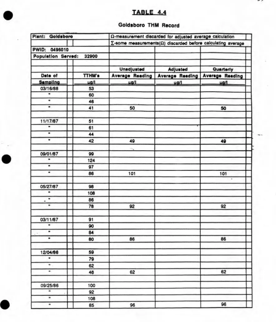
The THM record for each system was organized using a spreadsheet. The format

used for each record is shown in Tables 4.1, 4.2, 4.3 and 4.4, which are the THM

records for the Pasquatank County, Richmond County, Reidsville, and Goldsboro systems.

The name of the plant, the Public Water Supply Branch identification number, and the

number of persons served is indicated in the first few rows of the spreadsheet. The

records are arranged by the sampling date, which appears in the first column, beginning"

with the most recent data entry. The second column is used to designate those

measurements which were discarded, such as outliers, errors, and duplicates. These are

identified by an omega (Q) in the second column. Column 3 contains the individual total

trihalomethane measurements.

In Table 4.1, the first measurement on the 9/25/87 sampling date satisfied the

criteria for classification as an outlier, so it was discarded and an omega appears next to

it. The group of measurements appearing on the 9/1/87 sampling date in Table 4.1

were identified as duplicates, since they were identical to those measurements appearing

on 8/31/87. Accordingly, they were discarded. The same is true for the 6/22/87

entries, which were duplicates of the 6/18/87 entries. With the exception of one

measurement, the 5/7/86 entries are identical to the 2/13/86 entries. Because it is

32

TABLE 4.1

Pasquatank County THM Record

1 Plant: Pasquatank County

i £2-measurement discarded for adjusted average calculation

n

1

I-some measurements(n) discarded before calculating average |

PWID: 0470015

1 Population Served: 13000

1

1

Unadjusted Adjusted Quarterly

Date of TTHM'a Average Reading Average Reading

_{Average Reading |}

SamDilna ... ao/L ---uaa— Ufl/I _lUp/l

01/11/88 20

j

1 " 37

—1 **

60

I ** 67 46 46

09/25/87 a 144

1 ** 70

1 " 33

N

30 69 45

09/01/87 a 106

H a 76 • ** a 49 N

a 30 65

-. 08/31/87 30 n 49 ** 106

1 ** 76 65 56 I

06/22/87 a 73

**

a 53

N

a 42

"

a 21 47

—j

06/18/87 21

**

73

1 ** 42

"

53 47

47

—j

10/20/86 29

1 ** 42

1 ** 20

"

137 57

33

TABLE.

UL (cont'd)

Unadiuatad Adjuatad Quartarly

1 Data of

TTHM'a Avaraga Raading

1 Avaraga Raading

1 Avaraga Raading

1 SamollJ)a__ ug/l iia/1 ua/l UJ/I

r 08/29/86 23

8 70

88 47

07/07/86 30

1 ** 51

1 ** 61

1 ** 75 55 51

05/07/86 a 66

1 ** a 51

1 H _{a 51}

r " a 11 45

02/13/86 11

H

51

1 ** 44

**

66 "43 43

07/26/85 a 14

n

a 48

"

a 50

**

a 87 50

^

07/15/85 48

»

14

**

50

34

TABLE 4.2

Richmond County THM Record

1 Plant: Richmond County

_{^-measurement discarded for adjusted average calculation f 1}

I-some measurements(£2) discarded before calculating average ]

PWID: 0377109

1 Population Served: 13000

Unadjusted Adjusted Quarterly

Date of TTHM'e _{Average Reading Average Reading Average Reading}

Sampllny ug/l _atf/l uo/l ua/1

05/12/88 92

"

44 1 ** ₅₁

If

56 61 61

02/18/88 35

*'

24 1 ** 25

1 ** ₃₅ 30 30

ͣ

•

12/08/87 59

**

71

**

60

1 M

72 65

10/20/87 45

i ** 73 _J

'*

a 147

II

122 97 80 72 s

07/01/87 79

1 II

88

N

103

1 ** 90 90 90

03/31/87 97

1 ** 36

1 It ₅₆

1 ** _{a 114} 76 63 63

IJ

12/10/86 52

1 '* 47

"

84

35

TABLE 4.2 (cont'd)

Unadjusted Adjusted Quarterly

^^

Date of TTHM'e Average Reading Average Reading Average Reading

Sampling Ufl/l lifl/l Ufl/I u^/l

09/16/86 80

I*

101

*'

ci 207

1 " 132 130 104 104 I

1

06/23/86 59

1 *• 71

1 *' a 123

1 ** 65 79 65 65 I

03/21/86 49

1 H

39 H

50

H

77 54 54

12/19/85 67

1 H

49

1 ** 70 .

TABLE 4.3

Reidsviile THM Record

36

1 Plant: Reidsviile

£2-measurement discarded for adjusted average calculation { 1

I-some measurements(n) discarded before calculating average j

PWID: 0279020

1 Population Served: 13000

Unadjusted Adjusted Quarterly

Date of TTHM'e

_{Average Reading}

_{Average Reading}

Average Reading

1___Sampling___

ug/i ua/l _ug/l ua/l

03/16/88 30

**

35

-1 ** 34

**

41 35 35

12/08/87 34

ͣ

1 H ₃₄

1 ** 44

**

38 37 37

09/28/87 a 62

1 *• a 65

n

a 75

[... ...

H

a 78 70

09/03/87 62

" *'

65

*'

75

1 *' 78 70

07/31/87 a 76

1 ** _a 76 1 ** _Q 77

t «f

a 73 75 70

06/04/87 73

1 ** 76

1 " 77

1 ** 76 75 75

03/19/87 36

1 " 28 1 '* 26

TABLg 4.3 (cont'd)

37

Unadjuatad Adjuatad Quart ariy

^^^

Dat* of TTHM'a _{Avaraga Raading} Avaraga Raading Avaraga Raading

Sampling

iifl/1 u^l ua/l U9/I

11/25/86 33

1 ** 28

tl

33

I H 32 31 31

08/27/86 43

1 ** 39

[ ** 42

N

49 43 43

05/29/86 46

ft

39

H

52

1 ** ₅₄ 48

04/03/86 43

[ ** 52

M

50

1 ** 42 47 47

12/03/85 45 ^

1 ** 55

1 ** 25

1

51 44 44

09/03/85 77

1 ** 80

H

89

H

72 79 79

05/21/85 63

1 ** 71

1 ** 70

1 ** 50 63 63

03/19/85 32

1 ** 29 1 *' 42

38

TABUE 4.3 (cont'd)

Unadjuatad Adjuatad Quartarly ~^

Data of TTHM'a _{Avaraga Raading} Avaraga Raading Avaraga Raading

Samollnq Ufl/I uo/l _{.if/i "^f"}

08/02/84 65

**

77

-It

57

1 ** 69 67 67

05/15/84 52

H

48

**

46

1 ** 49 49 49

01/10/84 21

1 ** 32 1 ** 25

M

23 25 25

10/14/83 73

**

101

1 ** 88

1 ** 87 87 87

06/15/83 123

H

140

1 ** 132

1 II

139 133 133

"02/09/83 88 1 ** 79 1 *' _{a 104}

39

TABLE 4.4

Goldsboro THM Record

Plant: Goldsboro

n-measurement discarded for adjusted average calculation | |

Z-some measurements(n) discarded before calculating average

PWID: 0496010 1

Population Served: 32900

Unadjusted Adjusted Quarterly

Date of TTHM'8

_{Average Reading}

Average Reading Average Reading

Sumpllna ug/l liO/l ua/l ---ua/l

03/16/88 53

1

H

60

n

46

1 ** 41 SO 50

11/17/87 51

1 ** 61

H

44

1 " 42 49 49

09/01/87 99

H

124

**

97

1 H _{86 101} 101

-05/27/87 98

H

108

H

86

H

78 92 92

03/11/87 91

n

90

1 ** 84

** ₈₀ 86 86

12/04/86 59

**

79

'*

62

1 ** 48 62 62

09/25/86 100

1 ** 92 1 ** 108

TABLE 4.4 (confd)

kO

Unadjuatad Adjuatad Quartarly

^^n

Data of TTHM'a _{Avaraga Raading} Avaraga Raading Avaraga Raading

SamDlIn? iia/l ua/l Ufl/I

}^9'^ 06/03/86 97 If 109 ** 95 "

88 97 97

03/19/86 74 ** 87 H 71 M

68 75 75

12/05/85 a 113

H

65

M

58

1 ** 68 76 64 64

zl

09/20/85 83 •

1 ** 95 t

1 ** ₈₅

H

65 82 82

04/16/85 59

**

92

II

68

1 1*

63 70 70

02/07/85 50

H

58

H

53

1 It _{46 52} 52

12/18/84 58

1 " 71

M

50

1 H _{52 58} 58

09/18/84 96

II

112

1 " 94

II

TABLE 4.4 (cont'd)

41

Unadjustad Adluatad Quartarly

Data of TTHM'a Avaraga Raadlng Avaraga Raadlng Avaraga Raadlng

SamplliKf

ua/l ug/l ua/l ii^/l

05/03/84 96

"

114

**

73

1 If

88 93 93

03/06/84 100

*'

100

**

100

II

100 100 100

11/22/83 73

**

80

H

75 1 ** 62 1 ** a 73

H

a 80

II

a 75

1 II

a 62 72 72 72

n

06/21/83 50

II

93

H

75

H

84 75 75

03/10/83 124

"

111

ti

116

II

n 162 128 117

- 01/18/83 112

H

142

**

94

H

kZ

7/26/85 entries were identical to the 7/15/85 entries, these were also identified as

duplicates and discarded.

in Table 4.2, outliers were identified on the 10/20/87, 3/31/87, 9/16/86,

and 6/23/86 sampling dates. These measurements, designated by an omega (Q.)

appearing next to them, were discarded.

In Table 4.3, the entries appearing on the 9/28/87 sampling date were discarded

since they were identified as duplicates of the entries appearing on 9/3/87. The entries

appearing on 7/31/87 were also discarded as duplicates because they were identical to

the entries appearing on 6/4/87. One of the entries on the 2/9/83 sampling date

satisfied the criteria for classification as an outlier, so it was discarded.

In Table 4.4, the 12/5/85 and the 3/10/83 sampling dates each had one entry

which was discarded after it was identified as an outlier. Two identical sets of four

entries appear on the 11/22/83 sampling date, so four of the entries were discarded as

duplicates.

The Unadjusted Average, which is the average of all measurements taken on the

indicated sampling date, appears in column 4. The average of measurements taken on a

given sampling date, excluding all discarded measurements, appears in column 5. This

is the Adjusted Average and is computed only for those sampling dates where outliers

have been discarded. For example, on the 1/11/88 sampling date on Table 4.1, no

outliers were discarded, so an Adjusted Average did not have to be computed. An Adjusted

Average is computed for the 9/25/87 sampling date, since one of the values was

discarded as an outlier. A comparison of the Adjusted and Unadjusted Averages gives an

indication of the impact of discarded outliers.

^3

2.9 percent of the total number of entries. The number of low outliers and high outliers

was fairly evenly distributed, with 61 low outliers and 71 high outliers identified.

The Quarterly Average, appearing in column 6, is the average of all

measurements taken in a given quarter, excluding measurements discarded as outliers.

If any measurements taken during the quarter were discarded as outliers, a sigma (Z)

appears in column 7, next to the Quarterly Average. For example, one of the twelve

measurements taken during the third quarter (months 7, 8, and 9) of 1987 in the

Pasquatank County record (Table 4.1) was discarded as an outlier. The Quarterly

Average was computed for the remaining eleven measurements.

The Quarterly Average values were used for further analysis in computing the.

Two-Year Mean THM concentrations for each system and for preparing. graphical

representations of the data. Substitute Quarterly Average values were used for quarters

in which there was no data. The Pasquatank County record can be used to demonstrate the

method of substitution. It can be seen from Table 4.1 that no data exists in the

Pasquatank County record for the fourth quarter of 1987, the first quarter of 1987, and

the fourth quarter of 1985. The second quarter of 1986 was also considered to have no

data since all entries for the quarter were discarded because they were identified as

duplicates. In order to provide a continuous sequence of Quarterly Average values, these

gaps in the record were filled by reasonable substituted values. When these gaps

occurred, the Quarterly Average value for the same quarter of the previous, year was

substituted. For instance, the Quarterly Average from the fourth quarter of 1986 was

substituted for the missing value in the fourth quarter of 1987. Similarly, the gap in

the first quarter of 1987 was filled by the Quarterly Average value from the first

ki^

measurements were discarded as duplicate values. No data from the second quarter of a

previous year was available, so the Quarterly Average from the same quarter of the

following year (second quarter of 1987) was used.

Once the eight values representing the Quarterly Average TTHM concentrations of

the most recent two years of data were assembled, the Two-Year Mean TTHM

concentration was computed by taking the average of the eight values.

A plot of the Quarterly Average TTHM concentrations versus the quarter sampled

for the Pasquatank County water system is shown In Figure 4.1. This graph represents

the adjusted data from Table 4.1. The substituted Quarterly Averages are designated by a

different symbol which appears in the legend. Figure 4.1 indicates that Quarterly

Average values did not vary substantially over the course of the year. By contrast,

Figure 4.2 for the Richmond County system, illustrates a substantial variation in

Quarterly Average TTHM concentrations and a more distinct seasonal pattern to the

variations, with peak values occurring in the third quarter, and minimum values

occurring in the first quarter. The Quarterly Average TTHM concentration plots for the

Reidsville and Goldsboro systems are shown in Figure 4.3 and 4.4.

Speadsheets and graphs of the Quarterly Average TTHM concentrations were

prepared for all 63 of the systems for which TTHM data were available. The

spreadsheets and graphs appear in Appendix A. The Two-Year Mean TTHM concentrations

do not appear on the individual spreadsheets, but are tabulated in Table 4.5 (see below).

Summary of Two-Year Mean TTHM Concentrations

^5

T H M s

ng/i 100.

90_ 80_ 70_ 60_

50. 40.

30. 20.

10.

0

H---1---\---\---1---1---h-3 4 1 2 H---1---\---\---1---1---h-3 4 1

'86 Quarter Sampled

o Quarterly average a Substituted quarterly average

H---\---V

1

'88

Figure 4.1

Quarterly Average TTHM Concentrations for the Pasquatank County System

H iig/l

Quarter Sampled

«Quarterly average a Substituted quarterly average

1

'88

Figure 4.2

—smmm^m.

46

T

H M s

150

135_

120

105_ 90_

^g/i 75

60_ 45_ 30_

15

T

H M W/l s

I I I I I I I I I i I I I I I i I I I I I

123412341234123412341

•84 Quarter Sampled '87

o Quarterly average a Substituted quarterly average

Figure 4.3

Record of Quarterly ͣ Average TTHM Concentrations for the Reidsville System

150_ 135_

120

105 90

75 60 45 30 15

0

I I I I I I I I I I I I I I I I I I I I I

123412341234123412341

'84 Quarter Sampled '87

o Quarterly average a Substituted quarterly average

Figure 4.4

^7

TABLE 4.5

Average TTHIVI Concentrations in North Carolina

Water Systems Two-Year Mean TTHM

System Location Concentration (aa/M Type of Source

Elizabeth City 314 Surface & Ground

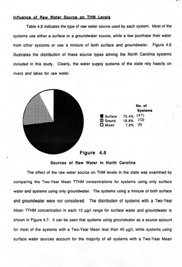
Rocl^y Mount 154 Surface

USMC-Cherry Point 101 Ground

Raleigh 94 Surface

Fayetteville 93 Surface

Southern Pines 93 Surface

Gary 91 Surface & Ground

Wilson 91 Surface

Wilmington 88 Surface

Sanford 87 Surface

Davidson 83 Surface

Goldsboro 82 Surface

King District 81 Surface

Durham 78 Surface

Lexington 78 Surface

Thomasville 78 Surface

CWASA 77 Surface

Asheboro 75 Surface

Roxboro 74 Surface

USMC-New River Air Station 74 Ground

High Point 70 Surface

Richmond County 68 Surface

-Winston-Salem 67 Surface

Anson County 65 Surface

Kannapolis 64 Surface

Monroe 64 Surface

Henderson-Kerr 63 Surface

Belmont 62 Surface

Burlington 62 Surface

Dunn 62 Surface

Morganton 62 Surface

Charlotte 60 Surface

Shelby 59 Surface

Davie County 58 Surface

Tarboro 55 Surface

Greenville 52 Surface & Ground

Albemarle 51 Surface

Greensboro 51

(continued)

48

TABLE 4.5 (cont'd)

Two-Year Mean TTHM

System Location Concentration. (Hfl/Q Tvpe of Source

Reidsville 51 Surface

Concord 50 Surface

Fort Bragg 50 Surface

Pasquatank County 50 Ground

Salisbury 49 Surface

Lenoir 46 Surface

Gastonia 45 Surface

Hickory 45 Surface

Statesville 45 Surface

Eden 44 Surface

Marion 44 Surface

Roanoke Rapids 43 Surface

Cape Fear Water Co. 42 Ground

Hendersonville 42 Surface

Jacksonville 38 Ground

Lumberton 38 Surface & Ground

Asheville 34 Surface

Waynesville 34 Surface

-New Bern 27 Ground

USMC-Hadnot Point (*) 26 Ground

Boone 25 Surface

Robeson County (*) 6 Surface & Ground

Laurinburg 2 Ground

Onslow County 2 Ground

Brookwood 6 Ground

Garner eo Purchased

Kinston 1 Ground

Pamlico County 8 Ground

Union County £ Purchased

(*) - Two Year Mean is basedon less than two years of data. S - Record was not found in the database.

« - Water is purchased from

Raleigh system; no THM values

reported.

§ - Less than one year of data

was available.