244
A hybrid metaheuristic algorithm for the robust pollution-routing
problem
Reza Eshtehadi
1, Mohammad Fathian
1∗, Mir Saman Pishvaee
1, Emrah Demir
21School of Industrial Engineering, Iran University of Science and Technology, Tehran, Iran
2The Panalpina Centre for Manufacturing and Logistics, Cardiff Business School, Cardiff University, Cardiff, United Kingdom
[email protected]; [email protected]; [email protected], [email protected]
Abstract
Emissions resulted from transportation activities may lead to dangerous effects on the whole environment and human health. According to sustainability principles, in recent years researchers attempt to consider the environmental burden of logistics activities in traditional logistics problems such as vehicle routing problems (VRPs). The pollution-routing problem (PRP) is an extension of the VRP which consists of routing a number of vehicles to serve a set of customers and determining their speed on each route segment so as to minimize a function of comprising fuel, emissions and driver costs. This paper proposes an adaptive large neighborhood search for the robust PRP (RPRP) under demand uncertainty. The achieved results indicate a premium performance of the solutions obtained by the proposed robust models.
Keywords:Green vehicle routing, pollution-routing problem, robust optimization, metaheuristic algorithm
1- Introduction
Green vehicle routing is related to dispatching goods not only based on economic goals, but also by considering the relevant harmful impacts on the environment (Sbihi and Eglese 2007). Transportation has dangerous effects on the environment such as resource depletion, land use, acidification, toxic effects on ecosystems and humans, noise and the impacts induced by Greenhouse Gas (GHG) emissions (Knörr, 2008; Kwon et al., 2013). GHGs and in particular, CO2-equivalent emissions are
the most disturbing matters about the environment in the last decade (Bektaş and Laporte, 2011; Li et al., 2015).
As vehicle planning has a significant effect on the environment and GHG emissions; a number of authors (e.g.,McKinnon, 2007; Sbihi and Eglese, 2007; Lee et al., 2014) mention that there are several opportunities for reducing GHG emissions by developing the classical VRP objectives to account for environmental and social burdens rather than just considering the economic profit (Bektaş and Laporte, 2011).
The Vehicle Routing Problem (VRP) is a well-known NP-hard problem which was firstly introduced by Dantzig and Ramser (1959). Since that time, VRP has been a topic of numerous studies
*Corresponding author
ISSN: 1735-8272, Copyright c 2018 JISE. All rights reserved
Journal of Industrial and Systems Engineering
Vol. 11, No. 1, pp. 244-257 Winter (January) 2018
245
in the literature of operations research. The traditional VRP includes a set of customers with known demands, a depot and a fleet of vehicles by objective of determining the optimized routes to minimize the total travel cost. The literature on VRP and its variants are very widespread and include many different models and extensions (see for example the latest surveys by Golden et al., 2008; Eksioglu et al., 2009; De Jaegere et al., 2014). Also various exact (e.g. Drexl 2014; Almoustafa et al., 2013; Baldacci et al., 2012;Dabia et al.;2017) and heuristics (e.g. Demir et al., 2012; Demir et al., 2014; Kopfer et al., 2014;Franceschetti et al.,2017) solution methods are suggested to solve these problems. In the real-word applications the input data of VRP is highly tainted with uncertainty. Therefore, several studies accomplished in this field and proposed mathematical approaches in order to handle the imprecision of input parameters in VRP. For example, Gendreau et al. (1996) illustrated different types and solution approaches for stochastic VRP (SVRP). The most common variant of SVRP is the VRP with stochastic customer demand. There are two main approaches in the literature for dealing with uncertain parameters in VRP: (1) stochastic programming which has been extensively applied in the condition that the probability distribution of the uncertain parameter is available according to sufficient and reliable historical data (e.g.Li et al., 2010;Juan et al., 2011), and (2) robust optimization which firstly used by Bertsimas and Simchi-Levi(1996) for SVRP and mostly applied when the probability distribution of uncertain parameter is unknown (i.e., deep uncertainty).
Sungur et al. (2008) introduced a robust optimization approach to solve the capacitated VRP (CVRP) with uncertain demand and compared the performance of robust solutions to deterministic ones. Adulyasak and Jaillet (2015) described a number models and algorithms for stochastic and robust vehicle routing problem (RVRP).
Green vehicle routing problem (GVRP) which was principally probed since 2006, is characterized by the objective of accounting of environmental burdens in addition to the economic costs (Lin et al., 2014). Lin et al. (2014) illustrated the three major directs of GVRP in their survey which includes GVRP, Pollution Routing Problem (PRP), and VRP in reverse logistics. The objective of PRP is to determine the vehicles path with less pollution. Demir et al. (2014) described main effective factors in fuel consumption and variant fuel consumption models in their review paper.
Despite the fact that the number of researches on PRPs is increasing in recent years, the studies are still restricted and have not covered many needed aspects. The uncertainty of input data, such as uncertain demand or travel time, is one of the important properties of real world problems. Many reasons like inventory fluctuations and customer interests may lead to demand uncertainty. Also any daily usual events can cause travel time uncertainty, such as road traffic, road accident and weather conditions. Eshtehadi et al. (2017) proposed several robust optimization models for the robust pollution routing problem (RPRP) regarding the PRP with uncertain demands (PRPUD) involve Hard worst case model, soft worst case model and chance constraint model. They show that the classical hard worst case approach commonly used for VRP, cannot achieve the right worst case solution of PRP. In this paper, we propose a solution method based on an enhanced adaptive large neighborhood search (ALNS) and a specialized speed optimization algorithm described in Demir et al. (2012) for the worst case robust PRP model is introduced by Eshtehadi et al. (2017). The results of adapted algorithm can show the effect of demand uncertainty in large scale instance and help decision makers to choose more suitable models in different uncertainty level.
The rest of this paper is organized as follows. In section 2,the Robust Pollution-Routing Problem is described and the related mathematical model is presented. Section 3 includes a brief description of the metaheuristic algorithm. The results of extensive numerical experiments presented in section 4. Finally, Section 5 concludes this paper and introduces some future research directions.
2- The robust pollution-routing problem
In this section the RPRP is described and the corresponding mathematical model is presented based on Eshtehadi et al. (2017) as the foundation of the proposed robust PRP models.
2-1- Problem description
The PRPUD is defined on a complete directed graph 𝐺𝐺= (𝑉𝑉,𝐴𝐴)with𝑉𝑉 = {0,1,2, … ,𝑛𝑛}as the set of nodes that node 0 considered as depot.𝐴𝐴= {(𝑖𝑖,𝑗𝑗):𝑖𝑖,𝑗𝑗 ∈ 𝑉𝑉,𝑖𝑖 ≠ 𝑗𝑗} is the set of arcs and the distance from node i to node j is shown by 𝑑𝑑𝑖𝑖𝑖𝑖. The number of homogeneous vehicles is a deterministic
246
exogenous parameter and set of vehicles is represented by𝑘𝑘= {1,2, … ,𝑚𝑚} and the capacity of each vehicle is equal to Q.
The tilde (~), bar (−) and hat (^) accents are distinguish the uncertain parameters, nominal value (which is used in deterministic modeling) and uncertain part of each uncertain parameter respectively; therefore, 𝑞𝑞�𝑖𝑖 is a uncertain parameter which is donated to customers demand with nominal value of 𝑞𝑞�𝑖𝑖 and maximum perturbation of 𝑞𝑞�𝑖𝑖 over and under nominal value (𝑞𝑞�𝑖𝑖𝑖𝑖uncertainty interval is �𝑞𝑞�𝑖𝑖𝑖𝑖−
𝑞𝑞�𝑖𝑖𝑖𝑖,𝑞𝑞�𝑖𝑖𝑖𝑖+𝑞𝑞�𝑖𝑖𝑖𝑖�). Uncertain demand results from a mixture of reasons such as some variation in customer interests, modes, styles and requirements as well as the number of them and their strategies. These factors may lead in undulation in real customer demand to expectations.
2-1-1- Diesel fuel consumption and CO2 emissions
The PRP model is introduced by Bektaş and Laporte (2011) based on the comprehensive emission models presented by Barth and Boriboonsomsin (2008), Barth et al. (2005) and Scora and Barth (2006). Later, Demir et al. (2012) have proposed a more useful formulation for fuel consumption rate that can be applied appropriately in PRP models. In this formulation the fuel consumption rate is calculated as the following:
(1)
𝐹𝐹(𝑣𝑣) =𝜆𝜆(𝐾𝐾𝐾𝐾𝑣𝑣+𝑤𝑤𝑤𝑤𝑤𝑤𝑣𝑣+𝑤𝑤𝑤𝑤𝛾𝛾𝑣𝑣+𝛽𝛽𝑤𝑤𝑣𝑣3)𝑑𝑑/𝑣𝑣
Where 𝑣𝑣,𝜏𝜏,𝜃𝜃,𝑑𝑑 and 𝑤𝑤 denote the vehicle speed, amount of acceleration, road angle, distance, and curb weight of an empty vehicle, respectively. Moreover, f denotes the vehicle load and α,𝛽𝛽,𝜆𝜆 and 𝑤𝑤 are constants which their formulations are as follows:
𝑤𝑤=𝜏𝜏+𝑔𝑔𝑔𝑔𝑖𝑖𝑛𝑛𝜃𝜃+𝑔𝑔𝐶𝐶𝑟𝑟𝑐𝑐𝑐𝑐𝑔𝑔, (2)
𝛽𝛽= 0.5𝐶𝐶𝑑𝑑𝜌𝜌𝐴𝐴, (3)
𝜆𝜆=𝜉𝜉/𝑘𝑘𝑘𝑘, (4)
𝑤𝑤= 1/1000𝑛𝑛𝑛𝑛𝑛𝑛𝑡𝑡𝑡𝑡. (5)
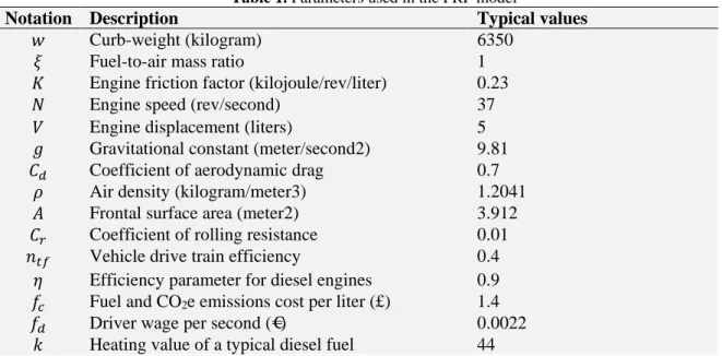
The definition of all parameters and their typical values are given in Table 1 based on Eshtehadi et al. (2017). The cost of fuel and CO2 emissions can be estimated as C=𝐹𝐹(𝑣𝑣)𝛾𝛾𝑐𝑐, where 𝛾𝛾𝑐𝑐 is the unit cost
of fuel and CO2 emissions.
Table 1. Parameters used in the PRP model
Typical values Description Notation 6350 Curb-weight (kilogram) 𝑤𝑤 1 Fuel-to-air mass ratio
𝜉𝜉
0.23 Engine friction factor (kilojoule/rev/liter)
𝐾𝐾
37 Engine speed (rev/second)
𝐾𝐾
5 Engine displacement (liters)
𝑉𝑉
9.81 Gravitational constant (meter/second2)
𝑔𝑔
0.7 Coefficient of aerodynamic drag
𝐶𝐶𝑑𝑑
1.2041 Air density (kilogram/meter3)
𝜌𝜌
3.912 Frontal surface area (meter2)
𝐴𝐴
0.01 Coefficient of rolling resistance
𝐶𝐶𝑟𝑟
0.4 Vehicle drive train efficiency
𝑛𝑛𝑡𝑡𝑡𝑡
0.9 Efficiency parameter for diesel engines
𝑛𝑛
1.4 (£)
emissions cost per liter e
2
Fuel and CO
𝛾𝛾𝑐𝑐
0.0022 Driver wage per second (€)
𝛾𝛾𝑑𝑑
44 Heating value of a typical diesel fuel
247 Typical values Description Notation (kilojoule/gram) 737 Conversion factor (gram/second to liter/second)
𝑘𝑘
5.55
(𝑐𝑐𝑜𝑜 20 𝑘𝑘𝑖𝑖𝑘𝑘𝑐𝑐 𝑚𝑚𝑚𝑚𝑚𝑚𝑚𝑚𝑜𝑜𝑔𝑔 ℎ𝑐𝑐𝑜𝑜𝑜𝑜⁄ ) Lower speed limit (meter/second)
𝑣𝑣𝑙𝑙
25 (𝑐𝑐𝑜𝑜 90 𝑘𝑘𝑖𝑖𝑘𝑘𝑐𝑐 𝑚𝑚𝑚𝑚𝑚𝑚𝑚𝑚𝑜𝑜𝑔𝑔 ℎ𝑐𝑐𝑜𝑜𝑜𝑜⁄ ) Upper speed limit (meter/second)
𝑣𝑣𝑢𝑢
2-2- The PRP Model formulation
In this section we present the model formulation for the PRP. Speed function should be discretized, that defined by R non-reducing speed levels𝑣𝑣̅𝑟𝑟(𝑜𝑜= 1,2, … ,𝑅𝑅) . Binary variables 𝑥𝑥𝑖𝑖𝑖𝑖are equal to 1 if arc (𝑖𝑖,𝑗𝑗) appears in solution.𝑧𝑧𝑖𝑖𝑖𝑖𝑟𝑟 is a binary variable equal to 1 if arc (𝑖𝑖,𝑗𝑗)∈ 𝐴𝐴 is crossed by a speed level r, and 0 otherwise. Continuous variables 𝛾𝛾𝑖𝑖𝑖𝑖 defined the total amount of flow on each arc. 𝑦𝑦𝑖𝑖is a non-negative continuous variable representing the time at that service starts at node 𝑗𝑗 ∈
𝐾𝐾0.Accordingly, the integer linear programming formulation of the PRP is shown in below:
(6)
𝑀𝑀𝑖𝑖𝑛𝑛𝑖𝑖𝑚𝑚𝑖𝑖𝑧𝑧𝑚𝑚 � �
𝛾𝛾𝑐𝑐𝑘𝑘𝐾𝐾𝑉𝑉𝜆𝜆𝑑𝑑𝑖𝑖𝑗𝑗�
𝑧𝑧𝑖𝑖𝑗𝑗𝑜𝑜�
𝑣𝑣�
𝑜𝑜𝑅𝑅 𝑜𝑜=1
+
� �
𝛾𝛾𝑐𝑐𝑤𝑤𝑤𝑤𝜆𝜆𝑤𝑤𝑖𝑖𝑗𝑗𝑑𝑑𝑖𝑖𝑗𝑗𝑥𝑥𝑖𝑖𝑗𝑗𝑛𝑛 𝑖𝑖=0 𝑛𝑛 𝑖𝑖=0 𝑛𝑛 𝑖𝑖=0 𝑛𝑛 𝑖𝑖=0
+
� �
𝛾𝛾𝑐𝑐𝑤𝑤𝜆𝜆𝑤𝑤𝑖𝑖𝑗𝑗𝑑𝑑𝑖𝑖𝑗𝑗𝛾𝛾𝑖𝑖𝑗𝑗𝑛𝑛 𝑖𝑖=0 𝑛𝑛 𝑖𝑖=0
+
� �
𝛾𝛾𝑐𝑐𝛽𝛽𝑤𝑤𝜆𝜆𝑑𝑑𝑖𝑖𝑗𝑗�
𝑧𝑧𝑖𝑖𝑗𝑗𝑜𝑜( 𝑅𝑅 𝑜𝑜=1 𝑛𝑛 𝑗𝑗=0 𝑛𝑛 𝑖𝑖=0𝑣𝑣
�
𝑜𝑜2)+
�
𝑔𝑔𝑖𝑖𝛾𝛾𝑑𝑑 𝑛𝑛 𝑖𝑖=0 Subject to:(7)
� 𝑥𝑥0𝑖𝑖 𝑛𝑛 𝑖𝑖=1
≤ 𝑚𝑚
(8)
∀𝑖𝑖 ∈ 𝐾𝐾0
� 𝑥𝑥𝑖𝑖𝑖𝑖 𝑛𝑛 𝑖𝑖=0
= 1
(9)
∀𝑗𝑗 ∈ 𝐾𝐾0
� 𝑥𝑥𝑖𝑖𝑖𝑖 𝑛𝑛 𝑖𝑖=0
= 1
(10)
∀𝑖𝑖 ∈ 𝐾𝐾0
� 𝛾𝛾𝑖𝑖𝑖𝑖 𝑛𝑛 𝑖𝑖=0,𝑖𝑖≠𝑖𝑖
− � 𝛾𝛾𝑖𝑖𝑖𝑖
𝑛𝑛 𝑖𝑖=0,𝑖𝑖≠𝑖𝑖
=𝑞𝑞𝑖𝑖
(11)
(𝑖𝑖,𝑗𝑗)∈ 𝐴𝐴 𝑞𝑞𝑖𝑖𝑥𝑥𝑖𝑖𝑖𝑖 ≤ 𝛾𝛾𝑖𝑖𝑖𝑖 ≤(𝑄𝑄 − 𝑞𝑞𝑖𝑖)𝑥𝑥𝑖𝑖𝑖𝑖
(12)
∀𝑖𝑖 ∈ 𝐾𝐾,∀𝑗𝑗 ∈ 𝐾𝐾0, i≠j 𝑦𝑦𝑖𝑖− 𝑦𝑦𝑖𝑖+𝑚𝑚𝑖𝑖+�
𝑑𝑑
𝑖𝑖𝑗𝑗𝑧𝑧
𝑖𝑖𝑗𝑗𝑜𝑜
𝑣𝑣
�𝑜𝑜 � 𝑅𝑅 𝑜𝑜=1≤ 𝐾𝐾𝑖𝑖𝑖𝑖�1− 𝑥𝑥𝑖𝑖𝑖𝑖�
(13)
∀𝑗𝑗 ∈ 𝐾𝐾0
𝑦𝑦𝑖𝑖− 𝑔𝑔𝑖𝑖+𝑚𝑚𝑖𝑖+�
𝑑𝑑
𝑗𝑗0𝑧𝑧
𝑗𝑗0𝑜𝑜
𝑣𝑣
�𝑜𝑜 � 𝑅𝑅 𝑜𝑜=1≤ 𝐿𝐿�1− 𝑥𝑥𝑖𝑖0�
(14)
∀𝑖𝑖 ∈ 𝐾𝐾0
𝑎𝑎𝑖𝑖 ≤ 𝑦𝑦𝑖𝑖 ≤ 𝑏𝑏𝑖𝑖
(15)
(𝑖𝑖,𝑗𝑗)∈ 𝐴𝐴
� 𝑧𝑧
𝑖𝑖𝑖𝑖𝑟𝑟=
𝑥𝑥𝑖𝑖𝑗𝑗𝑅𝑅 𝑟𝑟=1
(16)
(𝑖𝑖,𝑗𝑗)∈ 𝐴𝐴 𝑥𝑥𝑖𝑖𝑖𝑖∈{0,1}
(17)
(𝑖𝑖,𝑗𝑗)∈ 𝐴𝐴, r=1,2,…,R
𝑧𝑧
𝑖𝑖𝑖𝑖𝑟𝑟 ∈{
0,1}
248
(18)
(𝑖𝑖,𝑗𝑗)∈ 𝐴𝐴 𝛾𝛾𝑖𝑖𝑖𝑖≥ 0
(19)
∀𝑖𝑖 ∈ 𝐾𝐾0.
𝑦𝑦𝑖𝑖 ≥ 0
The objective function (6) minimizes the quantity of total fuel consumption is derived from (1) and drivers wage..Constraint (7) guaranteed that maximum used vehicles must less than available vehicles. Constraints (8) and (9) assure that each customer should be visited exactly one time through the tour. Constraint (10) defines the arc flows as well as eliminating the sub-tours. Constraint (11) enforces the capacity limitations on the load of each vehicle. Constraints (12) - (14), which𝐾𝐾𝑖𝑖𝑖𝑖 =
max {0,𝑏𝑏𝑖𝑖+𝑚𝑚𝑖𝑖+𝑑𝑑𝑙𝑙𝑖𝑖𝑖𝑖𝑖𝑖𝑖𝑖− 𝑎𝑎𝑖𝑖}and L is a large number, enforce the time window restrictions (𝑘𝑘𝑖𝑖𝑖𝑖)Is the minimum speed level. Constraints (15) ensure that only one speed level is selected for each arc. Finally, constraints (16) - (19) enforce the binary and non-negativity restrictions on decision variables.
2-3- The hard worst case (HWC) robust optimization approach
Stochastic programming is the most important classical approach to handle uncertainty in
optimization problems; however, sufficient and reliable historical data is a necessary requirement while applying this approach in order to find probability distribution of uncertain parameters. In spite of this requirement, in real world problems it is very hard and in some cases impossible to achieve accurate and reliable data. As an alternative in robust optimization (RO), the distribution of uncertain parameters is not needed to be known and only the range for each of them is required.As the pioneer in RO area, Soyster(1973)presented a conservative linear optimization model which considers the worst case condition of uncertain parameters. Two decades later, Ben-Tal and Nemirovski (1998, 2000) and Bertsimas and Sim (2003, 2004)came up with some less conservatism robust optimization approaches which are based on box+ellipsoidal and box+polyheadral uncertainty sets, respectively. In this section, two robust optimization models are developed in order to cope with PRPUD. First, a new hard worst case model is proposed and thereafter a soft worst-case robust optimization approaches presented for the PRPUD.
A solution of an optimization problem is called “robust” if it stays feasible for roughly all possible values of uncertain parameters (i.e., feasibility robustness) and also results in objective function values which have the least deviation from the planned optimal value for almost all possible values of uncertain parameters (i.e., optimality robustness) (Pishvaee et al. 2012). Therefore, robust optimization (RO) approach tries to enhance the performance of the obtained solutions in both feasibility and optimality robustness aspects. As Pishvaee et al. (2012) mentioned, various RO approaches can be classified in three main categories including (1) hard worst case, (2) soft worst case and (3) realistic approaches.
Among the aforementioned categories, the hard worst case (HWC) approach provides the maximum conservatism against uncertainty for the decision maker. In other words, the obtained solution from this approach is always feasible for all possible values of uncertain parameters. Regarding the value of objective function, this approach assures that the value of objective function never violates the optimal planned value. HWC models are applied in the fields namely logistics management and different problems in this context such as VRP.
Eshtehadi et al.(2017) proposed a hard worst case robust optimization modelfor PRPUD that used in this paper. They extended deterministic model to hard worst case robust by making the following changes:
249
(20)
𝑀𝑀𝑖𝑖𝑛𝑛𝑖𝑖𝑚𝑚𝑖𝑖𝑧𝑧𝑚𝑚 � �𝛾𝛾𝑐𝑐𝑘𝑘𝐾𝐾𝑉𝑉𝜆𝜆𝑑𝑑𝑖𝑖𝑗𝑗 �𝑧𝑧𝑖𝑖𝑗𝑗𝑜𝑜 𝑣𝑣�𝑜𝑜 � 𝑅𝑅 𝑜𝑜=1 𝑛𝑛 𝑗𝑗=0 𝑛𝑛 𝑖𝑖=0
+� �𝛾𝛾𝑐𝑐𝑤𝑤𝑤𝑤𝜆𝜆𝑤𝑤𝑖𝑖𝑗𝑗𝑑𝑑𝑖𝑖𝑗𝑗𝑥𝑥𝑖𝑖𝑗𝑗
𝑛𝑛 𝑗𝑗=0 𝑛𝑛 𝑖𝑖=0
+ � �𝛾𝛾𝑐𝑐𝑤𝑤𝜆𝜆𝑤𝑤𝑖𝑖𝑗𝑗𝑑𝑑𝑖𝑖𝑗𝑗𝛾𝛾′𝑖𝑖𝑗𝑗
𝑛𝑛 𝑗𝑗=0 𝑛𝑛 𝑖𝑖=0
+� �𝛾𝛾𝑐𝑐𝛽𝛽𝑤𝑤𝜆𝜆𝑑𝑑𝑖𝑖𝑗𝑗 �𝑧𝑧𝑖𝑖𝑗𝑗𝑜𝑜(
𝑅𝑅 𝑜𝑜=1 𝑛𝑛 𝑗𝑗=0 𝑛𝑛 𝑖𝑖=0 𝑣𝑣
�𝑜𝑜2)
+�𝑔𝑔𝑖𝑖𝛾𝛾𝑑𝑑 𝑛𝑛 𝑖𝑖=0
Subject to:
constraints (7) to (9), (12)to (19) and:
(21)
� 𝛾𝛾′
𝑖𝑖𝑖𝑖 𝑛𝑛 𝑖𝑖=0,𝑖𝑖≠𝑖𝑖
− � 𝛾𝛾′
𝑖𝑖𝑖𝑖 𝑛𝑛 𝑖𝑖=0,𝑖𝑖≠𝑖𝑖
=𝑞𝑞�𝑖𝑖+𝑞𝑞�𝑖𝑖 , 𝑖𝑖 = 1,2, … ,𝑛𝑛
(22)
𝛾𝛾′
𝑖𝑖𝑖𝑖 ≤(𝑄𝑄 − 𝑞𝑞�𝑖𝑖− 𝑞𝑞�𝑖𝑖)𝑥𝑥𝑖𝑖𝑖𝑖, ∀(𝑖𝑖,𝑗𝑗)∈ 𝐴𝐴
(23)
𝛾𝛾′
𝑖𝑖𝑖𝑖 ≥ �𝑞𝑞�𝑖𝑖+𝑞𝑞�𝑖𝑖�𝑥𝑥𝑖𝑖𝑖𝑖,∀(𝑖𝑖,𝑗𝑗)∈ 𝐴𝐴
(24)
𝛾𝛾0𝑖𝑖 ≤ 𝛾𝛾′0𝑖𝑖,𝑖𝑖= 1,2, … ,𝑛𝑛
(25)
� 𝛾𝛾𝑖𝑖𝑖𝑖 𝑛𝑛 𝑖𝑖=0,𝑖𝑖≠𝑖𝑖
− � 𝛾𝛾𝑖𝑖𝑖𝑖
𝑛𝑛 𝑖𝑖=0,𝑖𝑖≠𝑖𝑖
− � 𝛾𝛾′
𝑖𝑖𝑖𝑖 𝑛𝑛 𝑖𝑖=0,𝑖𝑖≠𝑖𝑖
+ � 𝛾𝛾′ 𝑖𝑖𝑖𝑖 𝑛𝑛 𝑖𝑖=0,𝑖𝑖≠𝑖𝑖
= 2𝑞𝑞�𝑖𝑖 , 𝑖𝑖= 1,2, … ,𝑛𝑛
(26)
𝛾𝛾′
𝑖𝑖𝑖𝑖 ≥0,∀(𝑖𝑖,𝑗𝑗)∈ 𝐴𝐴
Which continuous variables 𝛾𝛾′𝑖𝑖𝑖𝑖 defined the total amount of flow on arc(𝑖𝑖,𝑗𝑗). If each customer takes the lower bound value of demand parameter while the vehicle's load takes the upper bound value of demand, variable 𝛾𝛾𝑖𝑖𝑖𝑖 shows the total amount of flow on the arc(𝑖𝑖,𝑗𝑗). Moreover, if both customer and vehicle's load takes the upper bound value of demand parameters, then the load of vehicles in each arc should be computed in hard worst case condition. Constraint (21) defines the hard worst case arc flows as well as eliminating the sub-tours like Constraint (10). Constraints (22) to (24) enforce the capacity limitations on each vehicle. Constraint (25) ensures the flow balance according to relations between variables𝛾𝛾𝑖𝑖𝑖𝑖𝑎𝑎𝑛𝑛𝑑𝑑𝛾𝛾′𝑖𝑖𝑖𝑖.
3- An adaptive large neighborhood heuristic algorithm for the RPRP
As the main propose of this paper is analyzing the effect of uncertainty in RPRP,we use an enhanced version of the ALNS algorithm introduced by Demir et al. (2012) with the same parameters that results of computational experimentation confirmed the efficiency of them and we just adapted a part of algorithm for the RPRP. We describe the ALNS briefly here and refer the interested reader to Demir et al. (2012) for comprehensive details of this algorithm and parameters’ values.
The ALNS metaheuristic first proposed by Ropke and Pisinger (2006) as an extension of the large neighborhood search (LNS) heuristic introduced by Shaw (1998). Ropke and Pisinger (2006) used ALNS to solve variants of the VRP and shown the perfect efficiency of ALNS for these problems. ALNS algorithm based on the idea of improving an initial solution by means of some repair and destroy operators. In each iteration one removal operator, as destroy function, and one insertion operator, as repair operator, are chosen by roulette wheel mechanism according to their past performance. Repair operator inserting the nodes in the removal list, which removed by destroy operator from current solution, back into the routes. As like as Demir et al. (2012) we use the classical Clarke and Wright (1964) heuristic to construct an initial solution and the same 12 removal and five insertion operators in the ALNS algorithm. The new solution is accepted if it satisfies a criterion defined by the simulated annealing (Kirkpatrick, Gelatt, & Vecchi, 1983) used as local search framework used at the last loop. The score of used operators in each iteration updated regarding to
250
new solution objective function. At the end, the speed optimization procedure (SOP) is used for computing the optimal speed on each arc of the route in order to minimize objective function comprising fuel consumption and driving wage. This is the same algorithm as illustrated in Demir et al. (2012) that interested readers can refer.
4- Computational results
In this section the performance of the proposed robust models are investigated in 10, 50,100 and 200 nodes PRP data sets. Twenty instances of each groups of PRP library that are used to analyze the effect of the data uncertainty in RPRP based on hard worse case model. All the used instances are achievable from http://www.apollo.management.soton.ac.uk/prplib.htm. The computational experiments are conducted using Core i5 CPU 1.68 GHZ personal computer with 8 GB RAM.
4-1- Performance on RPRP instances
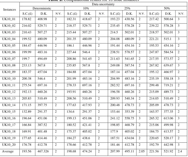
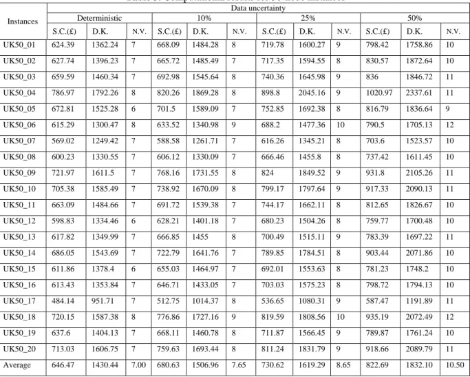
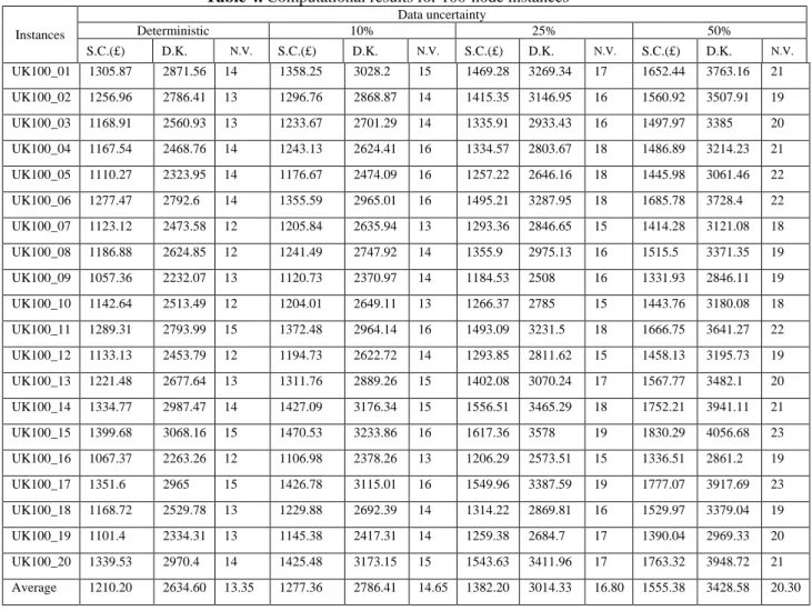
In tables 2 to 5, the results of different uncertainty levels are shown for each group of instances. Three levels of uncertainty (10, 25 and 50 percent) considered behind deterministic value to analyze the effect of uncertainty. For example, when using 10 percent uncertainty level, real demand for each customer changes between [0.9*nominal value, 1.1*nominal value].
We use three abbreviations in the tables. S.C. shows the Solution cost (£), D.K. used instead of total routes distances in kilometers, and finally N.V. shows the Number of used vehicles.
251
Table 2. Computational results for 10-node instances
Instances
Data uncertainty
Deterministic 10% 25% 50%
S.C.(£) D.K. N.V. S.C.(£) D.K. N.V. S.C.(£) D.K. N.V. S.C.(£) D.K. N.V.
UK10_01 178.82 408.98 2 182.31 418.67 2 193.23 430.56 2 217.42 500.64 3 UK10_02 216.02 529.71 2 218.37 529.71 2 235.45 578.28 2 239.22 578.28 3 UK10_03 210.43 507.27 2 215.44 507.27 2 214.5 502.01 2 218.57 502.01 3 UK10_04 199.52 480.09 2 201.35 480.09 2 204.08 480.09 2 221.21 515.1 3 UK10_05 184.47 446.96 2 186.1 446.96 2 191.44 454.16 2 195.53 454.16 2 UK10_06 199.99 483.16 2 227.44 546.4 2 238.51 578.57 2 247.87 584.54 2 UK10_07 199.7 494.69 2 208.86 541.65 2 211.63 541.65 2 217.55 573.57 2 UK10_08 233.13 567.8 2 235.85 567.8 2 249.08 587.54 2 267.82 639.67 3 UK10_09 183.37 457.04 2 184.88 457.04 2 187.14 457.04 2 195.12 466.97 2 UK10_10 200.38 546.4 2 201.99 483.16 2 204.99 483.16 2 235.19 558.18 3 UK10_11 275.54 697.16 2 278.33 697.16 2 282.52 697.16 2 299.48 719.21 2 UK10_12 192.13 460.26 2 193.91 460.26 2 196.58 460.26 2 215.09 489.73 2 UK10_13 205.83 510.49 2 208.56 510.49 2 209.93 540.34 2 214.05 510.49 2 UK10_14 171.15 397.75 2 177.63 417.93 2 200.48 478.73 2 205.09 478.73 2 UK10_15 132.89 291.37 2 134.6 291.37 2 153.44 353.39 2 163.57 377.35 2 UK10_16 196.64 451.06 2 199.13 451.06 2 241.12 558.75 3 265.32 613.06 3 UK10_17 166.84 387.52 2 180.52 421.41 2 198.85 468.79 2 215.06 499.98 2 UK10_18 169.91 401.48 2 175.37 405.02 2 177.9 405.02 2 184.75 413.57 2 UK10_19 177.65 414.46 2 184.27 438.6 2 187.51 434.04 2 220.65 520.17 2 UK10_20 176.78 412.78 2 178.66 412.78 2 181.46 412.78 2 192.79 442.98 3 Average 193.56 467.326 2 198.68 474.24 2 207.99 495.11 2.05 221.56 521.92 2.4
252
Table 3. Computational results for 50-node instances
Instances
Data uncertainty
Deterministic 10% 25% 50%
S.C.(£) D.K. N.V. S.C.(£) D.K. N.V. S.C.(£) D.K. N.V. S.C.(£) D.K. N.V.
UK50_01 624.39 1362.24 7 668.09 1484.28 8 719.78 1600.27 9 798.42 1758.86 10 UK50_02 627.74 1396.23 7 665.72 1485.49 7 717.35 1594.55 8 830.57 1872.64 10 UK50_03 659.59 1460.34 7 692.98 1545.64 8 740.36 1645.98 9 836 1846.72 11 UK50_04 786.97 1792.26 8 820.26 1869.28 8 898.8 2045.16 9 1020.97 2337.61 11 UK50_05 672.81 1525.28 6 701.5 1589.09 7 752.85 1692.38 8 816.79 1836.64 9 UK50_06 615.29 1300.47 8 633.52 1340.98 9 688.2 1477.36 10 790.5 1705.13 12 UK50_07 569.02 1249.42 7 588.58 1261.71 7 616.26 1345.21 8 703.6 1523.57 10 UK50_08 600.23 1330.55 7 606.12 1330.09 7 666.46 1455.8 8 737.42 1611.45 10
UK50_09 721.97 1611.5 7 768.16 1731.55 8 824 1849.52 9 931.8 2105.26 11
UK50_10 705.38 1585.49 7 738.92 1670.09 8 799.17 1797.64 9 917.33 2090.13 11 UK50_11 663.09 1484.66 7 691.72 1539.38 7 744.17 1662.11 8 812.65 1826.67 10 UK50_12 598.83 1334.46 6 628.21 1401.18 7 680.23 1504.26 8 759.77 1700.48 10 UK50_13 617.82 1349.99 7 666.85 1455 8 700.49 1515.11 9 783.39 1697.22 11 UK50_14 686.05 1543.69 7 722.79 1641.76 7 789.85 1784.51 8 903.44 2071.86 10 UK50_15 611.86 1378.4 6 655.03 1464.97 7 692.01 1553.63 8 781.23 1748.2 10 UK50_16 613.43 1353.84 7 646.71 1433.05 7 703.03 1575.23 8 798.72 1794.13 10 UK50_17 484.14 951.71 7 512.75 1014.37 8 536.65 1080.31 9 587.47 1191.89 11 UK50_18 720.15 1587.38 8 776.86 1727.16 9 819.59 1808.56 10 935.19 2072.49 12 UK50_19 637.6 1404.13 7 668.11 1460.78 8 711.87 1566.45 9 789.87 1761.24 10 UK50_20 713.03 1606.75 7 759.63 1693.44 8 811.24 1831.79 9 918.66 2089.79 11 Average 646.47 1430.44 7.00 680.63 1506.96 7.65 730.62 1619.29 8.65 822.69 1832.10 10.50
253
Table 4. Computational results for 100-node instances
Instances
Data uncertainty
Deterministic 10% 25% 50%
S.C.(£) D.K. N.V. S.C.(£) D.K. N.V. S.C.(£) D.K. N.V. S.C.(£) D.K. N.V.
UK100_01 1305.87 2871.56 14 1358.25 3028.2 15 1469.28 3269.34 17 1652.44 3763.16 21 UK100_02 1256.96 2786.41 13 1296.76 2868.87 14 1415.35 3146.95 16 1560.92 3507.91 19 UK100_03 1168.91 2560.93 13 1233.67 2701.29 14 1335.91 2933.43 16 1497.97 3385 20 UK100_04 1167.54 2468.76 14 1243.13 2624.41 16 1334.57 2803.67 18 1486.89 3214.23 21 UK100_05 1110.27 2323.95 14 1176.67 2474.09 16 1257.22 2646.16 18 1445.98 3061.46 22 UK100_06 1277.47 2792.6 14 1355.59 2965.01 16 1495.21 3287.95 18 1685.78 3728.4 22 UK100_07 1123.12 2473.58 12 1205.84 2635.94 13 1293.36 2846.65 15 1414.28 3121.08 18 UK100_08 1186.88 2624.85 12 1241.49 2747.92 14 1355.9 2975.13 16 1515.5 3371.35 19 UK100_09 1057.36 2232.07 13 1120.73 2370.97 14 1184.53 2508 16 1331.93 2846.11 19 UK100_10 1142.64 2513.49 12 1204.01 2649.11 13 1266.37 2785 15 1443.76 3180.08 18 UK100_11 1289.31 2793.99 15 1372.48 2964.14 16 1493.09 3231.5 18 1666.75 3641.27 22 UK100_12 1133.13 2453.79 12 1194.73 2622.72 14 1293.85 2811.62 15 1458.13 3195.73 19 UK100_13 1221.48 2677.64 13 1311.76 2889.26 15 1402.08 3070.24 17 1567.77 3482.1 20 UK100_14 1334.77 2987.47 14 1427.09 3176.34 15 1556.51 3465.29 18 1752.21 3941.11 21 UK100_15 1399.68 3068.16 15 1470.53 3233.86 16 1617.36 3578 19 1830.29 4056.68 23 UK100_16 1067.37 2263.26 12 1106.98 2378.26 13 1206.29 2573.51 15 1336.51 2861.2 19 UK100_17 1351.6 2965 15 1426.78 3115.01 16 1549.96 3387.59 19 1777.07 3917.69 23 UK100_18 1168.72 2529.78 13 1229.88 2692.39 14 1314.22 2869.81 16 1529.97 3379.04 19 UK100_19 1101.4 2334.31 13 1145.38 2417.31 14 1259.38 2684.7 17 1390.04 2969.33 20 UK100_20 1339.53 2970.4 14 1425.48 3173.15 15 1543.63 3411.96 17 1763.32 3948.72 21 Average 1210.20 2634.60 13.35 1277.36 2786.41 14.65 1382.20 3014.33 16.80 1555.38 3428.58 20.30
254
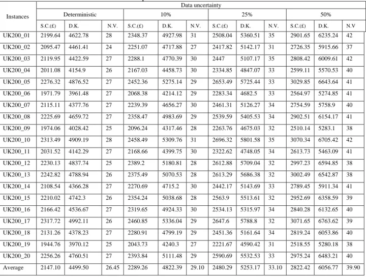
Table 5. Computational results for 200-node instances
Instances
Data uncertainty
Deterministic 10% 25% 50%
S.C.(£) D.K. N.V. S.C.(£) D.K. N.V. S.C.(£) D.K. N.V. S.C.(£) D.K. N.V
UK200_01 2199.64 4622.78 28 2348.37 4927.98 31 2508.04 5360.51 35 2901.65 6235.24 42 UK200_02 2095.47 4461.41 24 2251.07 4717.88 27 2417.82 5142.17 31 2726.35 5915.66 37 UK200_03 2119.95 4422.59 27 2288.1 4770.39 30 2447 5107.17 35 2808.42 6009.61 42 UK200_04 2011.08 4154.9 26 2167.03 4458.73 30 2334.85 4847.07 33 2599.11 5570.53 40 UK200_05 2276.32 4876.52 27 2452.36 5275.14 29 2653.49 5725.44 33 3029.85 6643.64 41 UK200_06 1971.79 3961.48 27 2068.38 4214.12 29 2283.34 4682.5 33 2564.97 5274.85 41 UK200_07 2115.11 4377.76 27 2239.39 4656.27 30 2461.31 5126.27 34 2754.59 5758.9 40 UK200_08 2225.69 4659.72 27 2358.47 4983.69 29 2539.59 5405.53 34 2902.51 6154.17 41 UK200_09 1974.06 4028.42 25 2096.24 4317.46 28 2263.76 4675.03 32 2510.14 5283.1 38 UK200_10 2313.49 4909.19 28 2458.49 5309.76 31 2696.32 5801.58 35 3070.34 6705.42 42 UK200_11 2031.52 4142.29 27 2168.66 4399.75 30 2322.62 4748.05 34 2613.73 5463.09 41 UK200_12 2230.13 4837.74 25 2389.2 5180.81 28 2612.88 5709.04 32 2997.23 6594.85 38 UK200_13 2242.82 4788.94 26 2375.49 5070.53 28 2613.29 5686.38 32 3002.49 6542.87 38 UK200_14 2108.54 4366.28 27 2270.69 4715.2 30 2442.17 5143.69 33 2789.45 5911.34 41 UK200_15 2210.02 4742.3 26 2354.24 5038.68 28 2563.9 5513.61 32 2952.69 6358.59 39 UK200_16 2166.42 4536.67 27 2319.65 4924.33 30 2534.13 5315.97 34 2840.28 6132.65 40 UK200_17 2317.72 4992.11 26 2460.85 5336.04 29 2647.6 5788.8 32 3071.65 6763.62 39 UK200_18 2131.26 4378.23 27 2280.91 4799.19 29 2451.36 5161.64 34 2819.24 6053.86 40 UK200_19 1944.76 3970.12 25 2043.73 4240.3 27 2221.67 4590.42 31 2518.55 5280.18 38 UK200_20 2256.26 4760.51 27 2393.84 5111.48 29 2590.69 5532.53 33 2975.24 6483.21 40 Average 2147.10 4499.50 26.45 2289.26 4822.39 29.10 2480.29 5253.17 33.10 2822.42 6056.77 39.90
Table 6 shows the summary of results for all instances. Each cell shows the average percent of increase in each factor in comparison with deterministic solution without uncertainty. For all test problems groups, the increase in uncertainty level caused in higher value of objective function, total distances and number of vehicles. Moreover, the effect of uncertainty is more observable in larger instances.
For 10-node instances, results show 14.47 percent increase in solution cost of maximum uncertainty level (50%) in comparison with deterministic solution cost, so decision makers should use robust solution with acceptable increase in their costs. But this amount increase to 31.45percent in average for 200-node instances and decision makers maybe want to choose other approaches with lower cost. The results show that data uncertainty in PRP, lead to significant increase in fuel consumption, driver wage and required fleet size, especially for large scale problems. In this situation, decision makers will have three choices to confront with this cost:
• Accept the risk of unmet demand cost and use deterministic models or soft worse case PRP models with less robustness level.
• Try to decrease data uncertainty level.
• Use any intelligent transportation system (ITS) as like as RFID (Radio-frequency identification) equipment for their fleet, and use Dynamic models or backup fleet for neutralize the effect of uncertainty.
If decision maker confronts with high uncertainty information and large scale problem, they should estimate the cost of each customer unmet demands and required ITS equipment for decrease uncertainty level, and then they can compare the surplus cost of robustness with two mentioned costs and choose the best solution.
255
Table 6. Summary of changes Percent relative to deterministic model
Instances
Data uncertainty
10% 25% 50%
S.C.(£) D.K. N.V. S.C.(£) D.K. N.V. S.C.(£) D.K. N.V.
10-node
instances 2.64 1.48 0.00 7.46 5.95 2.50 14.47 11.68 20.00
50-node
instances 5.28 5.35 9.29 13.02 13.20 23.57 27.26 28.08 50.00
100-node
instances 5.55 5.76 9.74 14.21 14.41 25.84 28.52 30.14 52.06
200-node
instances 6.62 7.18 10.02 15.52 16.75 25.14 31.45 34.61 50.85
Average 5.02 4.94 7.26 12.55 12.58 19.26 25.43 26.13 43.23
5- Conclusions
In this paper an adaptive large neighborhood search algorithm used for solving the Robust Pollution-Routing Problem. The ALNS algorithm adapted for hard worst case robust optimization PRP model and results of large scale instances data sets confirm the results of small size instances, that shown the direct relationship between objective function (involve fuel cost and driver wage) and data uncertainty level.
Results show necessity of using ITS systems for decrease the level of uncertainty and its effect, if the cost of unmet demands is high, or unacceptable. Otherwise decision makers should compare the cost of unmet demand and preparing intelligent fleet, or accept the cost of the RPRP solution.
References
Adulyasak, Y., & Jaillet, P. (2015). Models and Algorithms for Stochastic and Robust Vehicle Routing with Deadlines.Transportation Science,50(2),608-626
Almoustafa, S., Hanafi, S., & Mladenović, N. (2013). New exact method for large asymmetric distance-constrained vehicle routing problem. European Journal of Operational Research, 226(3), 386-394.
Baldacci, R., Mingozzi, A., & Roberti, R. (2012). Recent exact algorithms for solving the vehicle routing problem under capacity and time window constraints. European Journal of Operational
Research, 218(1), 1-6.
Barth, M., & Boriboonsomsin, K. (2008). Real-world carbon dioxide impacts of traffic congestion.
Transportation Research Record: Journal of the Transportation Research Board, 2058(1), 163-171.
Barth, M., Younglove, T., & Scora, G. (2005). Development of a heavy-duty diesel modal emissions and fuel consumption model.
Bektaş, T., & Laporte, G. (2011). The pollution-routing problem. Transportation Research Part B:
Methodological, 45(8), 1232-1250.
Ben-Tal, A., & Nemirovski, A. (1998). Robust convex optimization. Mathematics of Operations
256
Ben-Tal, A., & Nemirovski, A. (2000). Robust solutions of linear programming problems contaminated with uncertain data. Mathematical programming, 88(3), 411-424.
Bertsimas, D., & Sim, M. (2003). Robust discrete optimization and network flows. Mathematical
programming, 98(1-3), 49-71.
Bertsimas, D., & Sim, M. (2004). The price of robustness. Operations research, 52(1), 35-53.
Bertsimas, D. J., & Simchi-Levi, D. (1996). A new generation of vehicle routing research: robust algorithms, addressing uncertainty. Operations research, 44(2), 286-304.
Clarke, G., & Wright, J. W. (1964). Scheduling of vehicles from a central depot to anumber of delivery points. Operations Research, 12(4), 568–581.
Dabia, S., Demir, E., & Woensel, T. V. (2016). An exact approach for a variant of the pollution-routing problem. Transportation Science, 51(2), 607-628.
Dantzig, G. B., & Ramser, J. H. (1959). The truck dispatching problem. Management science, 6(1), 80-91.
De Jaegere, N., Defraeye, M., & Van Nieuwenhuyse, I. (2014). The vehicle routing problem: state of the art classification and review. FEB Research Report KBI_1415.
Demir, E., Bektaş, T., & Laporte, G. (2012). An adaptive large neighborhood search heuristic for the Pollution-Routing Problem. European Journal of Operational Research, 223(2), 346-359.
Demir, E., Bektaş, T., & Laporte, G. (2014). The bi-objective Pollution-Routing Problem. European
Journal of Operational Research, 232(3), 464-478.
Drexl, M. (2014). Branch‐and‐cut algorithms for the vehicle routing problem with trailers and transshipments. Networks, 63(1), 119-133.
Eksioglu, B., Vural, A. V., & Reisman, A. (2009). The vehicle routing problem: A taxonomic review.
Computers & Industrial Engineering, 57(4), 1472-1483.
Eshtehadi, R., Fathian, M., & Demir, E. (2017). Robust solutions to the pollution-routing problem with demand and travel time uncertainty. Transportation Research Part D: Transport and Environment, 51, 351-363.
Franceschetti, A., Demir, E., Honhon, D., Van Woensel, T., Laporte, G., & Stobbe, M. (2017). A metaheuristic for the time-dependent pollution-routing problem. European Journal of Operational Research, 259(3), 972-991.
Gendreau, M., G. Laporte, and R. Séguin, Stochastic vehicle routing. European Journal of Operational Research, 1996. 88(1): p. 3-12.
Golden, B. L., Raghavan, S., & Wasil, E. A. (2008). The Vehicle Routing Problem: Latest Advances
and New Challenges: latest advances and new challenges (Vol. 43): Springer.
Juan, A., Faulin, J., Grasman, S., Riera, D., Marull, J., & Mendez, C. (2011). Using safety stocks and simulation to solve the vehicle routing problem with stochastic demands. Transportation Research
Part C: Emerging Technologies, 19(5), 751-765.
Kirkpatrick, S., Gelatt, C. D., Jr., & Vecchi, M. P. (1983). Optimization by simulatedannealing. Science, 220(4598), 671–680.
257
Knörr, W. (2008). EcoTransIT: Ecological Transport Information Tool Environmental, Methodology and Data. Update.
Kopfer, H. W., Schönberger, J., & Kopfer, H. (2014). Reducing greenhouse gas emissions of a heterogeneous vehicle fleet. Flexible Services and Manufacturing Journal, 26(1-2), 221-248.
Kwon, Y. J., Choi, Y. J., & Lee, D. H. (2013). Heterogeneous fixed fleet vehicle routing considering carbon emission.Transportation Research Part D: Transport and Environment, 23,81-89.
Li, X., Tian, P., & Leung, S. C. (2010). Vehicle routing problems with time windows and stochastic travel and service times: models and algorithm. International Journal of Production Economics, 125(1), 137-145.
Li, H., Lv, T., & Li, Y. (2015). The tractor and semitrailer routing problem with many-to-many demand considering carbon dioxide emissions. Transportation Research Part D: Transport and
Environment, 34, 68-82.
Lin, C., Choy, K., Ho, G., Chung, S., & Lam, H. (2014). Survey of Green Vehicle Routing Problem: Past and future trends. Expert Systems with Applications, 41(4), 1118-1138.
McKinnon, A. (2007). CO2 Emissions from Freight Transport in the UK. Report prepared for the
Climate Change Working Group of the Commission for Integrated Transport.
Pishvaee, M., Razmi, J., & Torabi, S. A. (2012). Robust possibilistic programming for socially responsible supply chain network design: A new approach. Fuzzy sets and systems, 206, 1-20
Ropke, S., & Pisinger, D. (2006). An adaptive large neighborhood search heuristic forthe pickup and delivery problem with time windows. Transportation Science,40(4), 455–472.
Sbihi, A., & Eglese, R. W. (2007). Combinatorial optimization and green logistics. 4OR, 5(2), 99-116. Scora, G., & Barth, M. (2006). Comprehensive modal emissions model (CMEM), version 3.01. User
guide. Centre for Environmental Research and Technology. University of California, Riverside.
Soyster, A. L. (1973). Technical note—convex programming with set-inclusive constraints and applications to inexact linear programming. Operations research, 21(5), 1154-1157.
Sungur, I., Ordónez, F., & Dessouky, M. (2008). A robust optimization approach for the capacitated vehicle routing problem with demand uncertainty. Iie Transactions, 40(5), 509-523.