Using Cloud Computing for Solving Constraint
Programming Problems
Mohamed Rezgui??, Jean-Charles R´egin∗∗, and Arnaud Malapert∗∗ Univ. Nice Sophia Antipolis, CNRS, I3S, UMR 7271, 06900 Sophia Antipolis, France
Abstract. We propose to use cloud computing for solving constraint programing problems in parallel. We used the Embarrassingly Parallel Search (EPS) method in conjunction with Microsoft Azure, the cloud computing platform and infras-tructure, created by Microsoft. EPS decomposes the problem in many distinct subproblems which are then solved independently by workers. EPS has three ad-vantages: it is an efficient method, it is simple to deploy and it involves almost no communication between workers. Thus, EPS is particularly well-suited method for being used on cloud infrastructure. Experimental results show ratio of gain equivalent to those obtained for a parallel machine or a data center showing the strength of EPS while using in conjunction with a cloud infrastructure. We also compute the number of cores in a cloud infrastructure requires to improve the resolution by a factor ofkand we discuss about the price to pay for solving a given problem in a certain amount of time.
1
Introduction
Constraint Programming (CP) is an efficient method for solving complex optimization problems. In CP, problems are represented by variables subject to constraints on which combinations of values of variables are acceptable. Variables takes their values in do-mains and constraints are associated with filtering algorithms which aim at removing value that do not belong to a solution of the constraints. Efficient algorithms have been developed in CP for accelerating the search for a solution.
There are different way for improving the resolution of a problem. We can change the model or improving the internal algorithms. We can also use a more efficient proces-sor. In this paper, we are interested in the acceleration of the resolution by using more processors. More precisely, we would like to know the number of cores we should use to improve the resolution time by a factor ofp. This is not an easy task because usu-ally increasing the number of cores by a factor ofkdoes not mean that we increase the computational power by a factor ofk. There are several reasons: the parallelization must scale up and the communication must be reduced.
Several methods for parallelizing the search in constraint programming (CP) have been proposed. The most famous one is the work stealing [6,8,3,9,2,4]. This method uses the cooperation between computation units (workers) to divide the work dynami-cally during the resolution. Recently, [7] introduced a new approach named Embarrass-ingly Parallel Search (EPS), which has been shown competitive with the work stealing ??
method. EPS is simple and involve almost no communication so give us more chance to be able to predict the improvement that we can expect by usingkmore cores.
The idea of EPS is to decompose statically the initial problem into a huge number of subproblems that are consistent with the propagation (i.e. running the propagation mechanism on them does not detect any inconsistency). These subproblems are added to a queue which is managed by a master. Then, each idle worker takes a subproblem from the queue and solves it. The process is repeated until all the subproblems have been solved. The assignment of the subproblems to workers is dynamic and there is no communication between the workers. EPS is based on the idea that if there is a large number of subproblems to solve then the resolution times of the workers will be balanced even if the resolution times of the subproblems are not.
In other words, load balancing is automatically obtained in a statistical sense. In-terestingly, experiments of [7] have shown that the number of subproblems does not depend on the initial problem but rather on the number of workers. Moreover, they have shown that a good decomposition has to generate about30subproblems per worker. Experiments have shown good results on a multi-cores machine (40 cores/workers) and on a data center (512 cores/workers). The gain factor is clearly better with EPS than with work stealing when the number of cores is increased.
In this paper we study the behavior of EPS on a cloud infrastructure. Then, we establish some relations between the power different of type of machines and cloud computing. Since cloud computing is directly linked to price because we pay for using a machine having some features for a certain amount of time, we compare the price of a computation using cloud computing and the same computation using classical servers.
The paper is organized as follows. First we recall some preliminaries about con-straint programming and embarrassingly parallel method. Then, we give some exper-imental results when using EPS in conjunction with a cloud infrastructure. Next, we propose some relations between the power of a cloud computing approach and a more classical computing approach. At last, we conclude.
2
Preliminaries
A worker is a computation unit. Most of the time, it corresponds to a core. We will consider that there arewworkers.
2.1 EPS
The Embarassingly Paralell Search (EPS) method has been defined in [7]. This method splits statically the initial problem into a large number of subproblems that are consis-tent with the propagation and puts them in a queue. Once this decomposition is over, the workers take dynamically the subproblems from the queue when they are idle. Pre-cisely, EPS relies on the following steps:
• it splits a problem intopsubproblems such asp ≥ w and pushes them into the
queue.
• a master monitors the concurrent access of the queue. • the resolution ends when all subproblems are solved.
For optimization problems, the master manages the value of the objective. When a worker takes a subproblem from the queue, it also takes the best objective value com-puted so far. And when a worker solves a subproblem it communicates to the worker the value of the objective function. Note that there is no other communication, that is when a worker finds a better solution, the other workers that are running cannot use it for improving their current resolution.
The main strength of the method is the reduction of communication. Furthermore, a resolution in parallel can be replayed by saving the order in which the subproblems have been executed. This costs almost nothing and helps a lot the debugging of applications.
2.2 Constraint Programming
A constraint networkCN = (X,D,C)is defined by:
• a set ofnvariablesX ={x1, x2, . . . , xn}
• a set ofnfinitedomainsD={D(x1), D(x2), . . . , D(xn)}withD(xi)the set of
possiblevaluesfor the variablexi,
• a set ofconstraintsbetween the variablesC ={C1, C2, . . . , Ce}. A constraintCi is defined on a subset of variablesXCi={xi1, xi2, . . . , xij}ofXwith a subset of
Cartesian productD(xi1)×D(xi2)×. . .×D(xij), that states which combinations
of values of variables{xi1, xi2, . . . , xij}are compatible.
Each constraintCi is associated with a filtering algorithm that removes values of the domains of its variables that are not consistent with it. The propagation mechanism applies filtering algorithms of C to reduce the domains of variables in turn until no reduction can be done. For convenience, we will use the word ”problem” for designing a constraint network when it is used to represent the constraint network and not the search for a solution. We say that a problemP is consistent with the propagation if and only if running the propagation mechanism onPdoes not trigger a failure.
3
Cloud computing
3.1 Microsoft Azure Cloud
Microsoft Azure is a cloud infrastructure and Windows HPC is a high performance
computing (HPC) solution built on Windows Server technology (http://technet.microsoft.com/en-us/library/cc514029.aspx). It provides powerful computation units, named nodes, to the
user. Users may use different kind of nodes and hour of computation are bought. A node has between 1 and 8 cores. This is a choice of the user. This has no influence on the price or the power that are defined per core. Without loss of generality, we will consider only 8 cores nodes. When using nodes, some other management nodes must be
also bought. The rules are the following (http://technet.microsoft.com/en-us/library/jj899633.aspx):
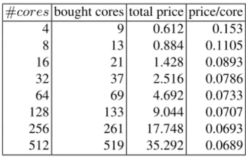
Table 1.Configuration: hourly price per available core #coresbought cores total price price/core
4 9 0.612 0.153 8 13 0.884 0.1105 16 21 1.428 0.0893 32 37 2.516 0.0786 64 69 4.692 0.0733 128 133 9.044 0.0707 256 261 17.748 0.0693 512 519 35.292 0.0689
– 2 hpcproxy nodes (each using 2 cores) are required up to 400 nodes.
– 1 hpcproxy node (using 2 cores) is required per additional 200 nodes
The hourly price per core is almost constant as shown in Table 1 (See https://azure.microsoft.com/en-us/pricing/details/virtual-machines/).
3.2 Experiments
Benchmark Instances All instances come from the minizinc distribution (see [5]). We report results for the twenty most significant instances we found. Two types of problems are used: enumeration problems and optimization problems.
Execution environment All the experiments have been made on three type of machines:
•cicada: the data center ”Centre de Calcul Interactif” hosted by the University of
Nice Sophia Antipolis. It has 1152 cores, spread over 144 Intel E5-2670 processors, with a 4,608GB memory and runs under Linux (http://calculs.unice.fr/ fr). We were allowed to use to up to 512 cores simultaneously for our experiments. The data center uses a scheduler (OAR) that manages jobs (submissions, executions, failures).
•fourmis: a Dell machine having four E7-4870 Intel processors, each having 10
cores with 256 GB of memory and running under Scientific Linux.
•azure: the Windows Azure cloud. We were allowed to use to up to 24 cores
simul-taneously for our experiments. We manage jobs with the Microsoft HPC Cluster 2012 (http://technet.microsoft.com/en-us/library/jj899572.aspx). Implementation EPS is implemented on the top of the solver gecode 4.0.0 [1]. We use MPI (Message Passing Interface), a standardized and portable message-passing system to exchange information between processes. Master and workers are MPI processes. Each process reads a FlatZinc model to init the problem and only jobs are exchanged through messages between master and workers.
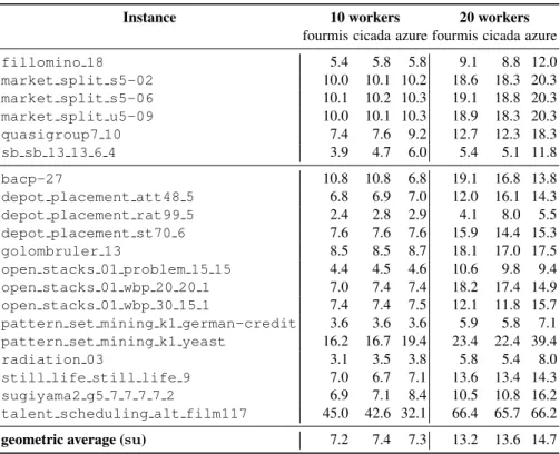
Scaling analysis We test the scalability of EPS for different numbers of workers with different machines and cloud infrastructure. Table 2 describe the details of the speedups
respectively on fourmis machine, cicada machine and Microsoft Azure (azure). We use the following definitions:
•t0is the resolution time of an instance in sequential •su= t0
t is the speedup of the overall resolution time compared with the sequential resolution time
Table 2.Scaling comparison between machines with EPS.
Instance 10 workers 20 workers
fourmis cicada azure fourmis cicada azure fillomino 18 5.4 5.8 5.8 9.1 8.8 12.0 market split s5-02 10.0 10.1 10.2 18.6 18.3 20.3 market split s5-06 10.1 10.2 10.3 19.1 18.8 20.3 market split u5-09 10.0 10.1 10.3 18.9 18.3 20.3 quasigroup7 10 7.4 7.6 9.2 12.7 12.3 18.3 sb sb 13 13 6 4 3.9 4.7 6.0 5.4 5.1 11.8 bacp-27 10.8 10.8 6.8 19.1 16.8 13.8 depot placement att48 5 6.8 6.9 7.0 12.0 16.1 14.3 depot placement rat99 5 2.4 2.8 2.9 4.1 8.0 5.5 depot placement st70 6 7.6 7.6 7.6 15.9 14.4 15.3 golombruler 13 8.5 8.5 8.7 18.1 17.0 17.5 open stacks 01 problem 15 15 4.4 4.5 4.6 10.6 9.8 9.4 open stacks 01 wbp 20 20 1 7.0 7.4 7.4 18.2 17.4 14.9 open stacks 01 wbp 30 15 1 7.4 7.4 7.5 12.1 11.8 15.7 pattern set mining k1 german-credit 3.6 3.6 3.6 5.9 5.8 7.1 pattern set mining k1 yeast 16.2 16.7 19.4 23.4 22.4 39.4 radiation 03 3.1 3.5 3.8 5.8 5.4 8.0 still life still life 9 7.0 6.7 7.1 13.6 13.4 14.3 sugiyama2 g5 7 7 7 7 2 6.9 7.1 8.4 10.5 10.8 16.2 talent scheduling alt film117 45.0 42.6 32.1 66.4 65.7 66.2 geometric average (su) 7.2 7.4 7.3 13.2 13.6 14.7
We observe that the scaling factor of the cloud infrastructure is comparable to the ones obtained with a parallel machine or with a data center.
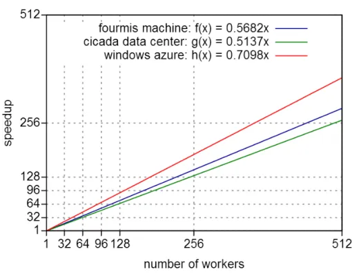
Performances comparison between machines Figure 1 describes the scaling func-tions for each machine up to 512 workers. For the Windows Azure cloud and fourmis machine, we extrapolate from their speedup because they do not have more cores than cicada machines (24 cores for Windows Azure and max 40 cores for fourmis machine). The scaling functions shows that Windows Azure has a better scaling than other ma-chines. However, these results have to be considered with caution.
Fig. 1.Scaling functions obtained by regression linear based on geometric speedup (all instances) with EPS for each machine up to 512 workers.
4
Resolution speed-up and resolution price
As mentioned in the introduction, it is not an easy task to improve the resolution of problem by a factor ofp, because it is not easy to use all the power provided by a core and because any code using several cores spend some times in computing an efficient way to use it as much as possible.
We can compute the number of cores required to increase by a factor ofpthe power of the machine usingkM cores. We define bysfM the scaling function for a machine
M. This is the value of the scaling of EPS for a given number of cores of the machine
M. Then, we search for the number of coresxsuch thatsfM(x) =p×sfM(kM), that isx=sfM−1(p×sfM(kM)). Thus we have,
Property 1 LetM be a machine. The number of cores needed to increase by a factor ofpthe power of machines when it useskM cores isx=sfM−1(p×sfM(kM))
4.1 Power equivalence
We propose to define a power equivalence between two machines, for instance a core on the Microsoft Azure cloud infrastructure and the core of a server machine. The idea
is to compute the number of cores for the machineM2that we need to have a practical
power equivalent to the power we have on a given machineM1.
Consider any machineM1usiingk1cores. We propose to computek2the number of
cores that we need on the machineM2to have a capacity of computation equivalent to
the one that we have with our machineM1. We say that two systems have an equivalent
capacity of computation if they requires exactly the same time for running the same program, that is for solving the same problem.
First, we define bypr(M1, M2)the performance ratio between two machines when
using only one core. An estimation of this number can be obtained by running a program on one core of each machine and by computing tM1
tM2
the ratio of the resolution times of each machine. For instance, for Microsoft Azure we obtaintA = 3167sand we measuredtF = 1355for the 40 cores machines so we havepr(A, F) = 3167/1355 = 2.34. On the data center, ie., the cicada machine, we measures the same time as for the 40 cores machine.
Then, we can compare two machines:
Property 2 LetM1andM2be two machines. Consider that the machineM1usesk1
cores. The number of cores k2 of the machine M2 needed for having an equivalent
power as thek1core on the machineM1is defined by:
k2=sfM−12(sfM1(k1)pr(M2, M1)) (1)
Consider the scaling function when using 20 cores. We observedsfA(x) = 0.7083x
for the Microsoft Azure cloud infrastructure,sfF(x) = 0.66for the forumis machine andsfC(x) = 0.68xfor Cicada, the data center. Thanks to Equaton eq1, Table 3 gives the number of cores for the fourmis and cicada machines for having a power equivalent to20cores on the Microsoft Azure cloud. Precisely, the number of cores for fourmis is equal to:sfF−1(sfA(20)pr(F, A)) =sfF−1(20×0.7083×1355/3167) =sf
−1
F (20× 0.7083×1355/3167) = 6,0609/0.66 = 9,19. The number of cores for cicada is equal to:sfC−1(sfA(20)pr(C, A)) =sfC−1(20×0.7083×1355/3167) =sf
−1
C (20× 0.7083×1355/3167) = 6,0609/0.68 = 8,92.
Table 3.Power equivalence of20Microsoft Azure cores Microsoft Azure cloud fourmis (server) cicada (data center)
#cores 20 9,19 8,92
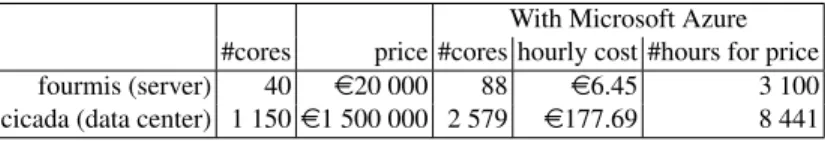
From the previous property and from Table 1 we can compute for the server ma-chine and for the data center, the number of hours of computations we can have on the Microsoft Azure cloud infrastructure with a number of cores leading to an equivalent power of the machines. Table 4 gives the results. We learn that the cost of an equivalent power of the data center corresponds to almost one year of computations on the cloud. Note that we do not integrate side cost like electricity or maintenance.
Table 4.Number of hours of computation for an equivalent power with the Microsoft Azure cloud infrastructure
With Microsoft Azure #cores price #cores hourly cost #hours for price fourmis (server) 40 e20 000 88 e6.45 3 100 cicada (data center) 1 150e1 500 000 2 579 e177.69 8 441
4.2 Price for a given power
We can make further computations and determine the price it will cost for obtaining a certain power computing during a certain time. This operation is useful for answering some question about the resolution of a problem within a given amount of time.
In other words, we would like to know how much it will cost to solve a problem with a machineM2in less thant2unit of time knowing that it requirest1unit of time
to be solve on a machineM1usingk1cores.
First, we define the number of cores needed to solve the problem with an equivalent power on the machineM2. From Equation 1 we havek2=sfM−12(sfM1(k1)pr(M2, M1)).
Then we need to increase the power by a factor oft1/t2. Property 1 gives us the answer.
So we have:
Property 3 LetM1 be a machine usingk1 cores for solving a problem int1units of
time. We can solve the problem with the machineM2int2 units of time by using the
numberk2of cores defined by
k2=sfM−12(t1/t2×sfM1(sf
−1
M2(sfM1(k1)pr(M2, M1)))) (2)
5
Conclusion
In this paper we have studied the behavior of th Embarrassingly Parallel Search method for solving constraint programming in parallel with cloud computing. Preliminaries re-sults have shown that the EPS methods scales on the Microsoft Azure cloud infrastruc-ture as well as it scales on a server or on a data center. This gave us the opportunity to define some properties establishing an equivalent power between infrastructures. This led us to define the cost of having an equivalent power with cloud computing as we can have with server machines or a data center.
References
1. Gecode 4.0.0. http://www.gecode.org/, 2012.
2. Geoffrey Chu, Christian Schulte, and Peter J. Stuckey. Confidence-Based Work Stealing in Parallel Constraint Programming. In Ian P. Gent, editor,CP, volume 5732 ofLecture Notes in Computer Science, pages 226–241. Springer, 2009.
3. Joxan Jaffar, Andrew E. Santosa, Roland H. C. Yap, and Kenny Qili Zhu. Scalable Distributed Depth-First Search with Greedy Work Stealing. InICTAI, pages 98–103. IEEE Computer Society, 2004.
4. Laurent Michel, Andrew See, and Pascal Van Hentenryck. Transparent Parallelization of Constraint Programming.INFORMS Journal on Computing, 21(3):363–382, 2009.
5. MiniZinc. http://www.g12.csse.unimelb.edu.au/minizinc/, 2012.
6. Laurent Perron. Search Procedures and Parallelism in Constraint Programming. In Joxan Jaf-far, editor,CP, volume 1713 ofLecture Notes in Computer Science, pages 346–360. Springer, 1999.
7. Jean-Charles R´egin, Mohamed Rezgui, and Arnaud Malapert. Embarrassingly parallel search. In Christian Schulte, editor, Principles and Practice of Constraint Programming, volume 8124, pages 596–610. Springer Berlin Heidelberg, 2013.
8. Christian Schulte. Parallel Search Made Simple. In ”Proceedings of TRICS: Techniques foR Implementing Constraint programming Systems, a post-conference workshop of CP 2000, pages 41–57, Singapore, 2000.
9. Peter Zoeteweij and Farhad Arbab. A Component-Based Parallel Constraint Solver. In Rocco De Nicola, Gian Luigi Ferrari, and Greg Meredith, editors,COORDINATION, volume 2949 ofLecture Notes in Computer Science, pages 307–322. Springer, 2004.