The Effect of U.S. Steel Antidumping Duties on Trade Patterns and Trade Diversion
By Jackson Trice
Senior Honors Thesis Economics Department
University of North Carolina at Chapel Hill
April 2020
Approved:
Acknowledgements
I would like to first thank my advisor, Dr. Patrick Conway, for the immense help and guidance that he has provided me throughout this process. By sharing his knowledge, I was able to expand my understanding of antidumping duties and trade diversion. Thanks to Dr. Conway’s guidance, I was able to construct a template of how antidumping duties impact trade, and
develop a methodology and model to calculate my results. Dr. Conway’s willingness to assist me was what made this thesis possible and I am very grateful for that.
I would also like to thank Dr. Jane Fruehwirth for helping both me and the entire class throughout the thesis process. I have not done anything like this before, but Dr. Fruehwirth made all the steps of the process very clear and was always willing to help in any way possible. She helped me stay on track and answered any questions that I had. I was able to learn about both the data and writing process of a thesis from her and that made a major difference when it came to completing this thesis.
I also want to thank the workers at the Odum Institute in Davis Library who help me with multiple data issues that I ran into. I especially want to thank Lauren and Will from the help desk who were able to answer any of my confusing questions and teach me many new data techniques in Stata. I would also like to thank Lakshita Jain, who took time out of her busy day to meet with me to fix a data problem I had been struggling with for days.
Abstract
This paper examines the impact of U.S. steel antidumping duties on trade patterns with both countries that are named on the duty and countries that are not named. The purpose of an antidumping duty is to punish the named dumping countries (companies) and reduce imports from them, which will help U.S. firms regain market share. The issue that arises from
1. Introduction
President Trump has greatly raised the visibility of U.S. tariff policy during his
presidency. The Trump Administration’s use of tariff policy is largely retaliatory, by imposing tariffs on countries, and firms in countries, whom he accuses of competing unfairly in
international markets. President Trump has imposed tariffs on many goods such as steel and aluminum. Producers from many countries are affected by these tariffs, such as the European Union, Canada, and Mexico. President Trump’s tariffs on China especially have escalated and led to a trade war between the two countries. His goal of the tariffs is to counteract the unfair advantages of foreign producers so that U.S. firms will face a level playing field.
While this has been a very active U.S. policy, it is difficult to assess how successful it has been. Success is defined as reducing trade with the accused country and improving the position of U.S. firms. In this paper, I examine the evidence from earlier U.S. use of retaliatory tariff policy on steel to judge what impact it has had on trade with the accused country. I also look to see whether the retaliatory tariffs led to an increase in steel imports from other non-accused countries, leaving the U.S. steel firms in a similar position compared to the international marketplace. By using an estimation that follows the format of an import function, I find that imported good from the accused country is reduced impacted by the duty. I also find an increase in steel imports from the non-accused countries, which means that trade diversion takes place.
steel antidumping duties may have been seen as a way to combat unfair trade with foreign steel companies and help U.S. steel firms regain market share. By focusing on U.S. steel antidumping duties, we examine whether they reduced imports from accused countries and helped domestic firms regain their market share.
The layout of this paper will proceed as follows. The market implications of tariff policy are discussed in section 2. Literature on how to measure the effects of retaliatory tariffs is
presented in section 3. The data, empirical model, and results of this paper are detailed in section 4. Lastly, the conclusions drawn from this paper and possible extensions from this paper are discussed in section 5.
2. Market implications of tariff policy
Commercial Policy
Commercial policy is an umbrella term that is used to describe government interventions to influence the pattern and volume of international trade. There are different types of trade policies that could be used to achieve either trade expansion or trade compression (Appleyard & Field, 2013). Trade expansion policies would be used to help incentivize trade between
countries. Some examples of this kind of policy are import and export subsidies. Trade
compression policies are the opposite of trade expansion policies, since they are used to decrease trade between countries. Import tariffs would fall into this category of commercial policy.
Goals of import tariffs
government treasury. Many developing countries have used import tariffs as a way of generating revenue. Another goal of an import tariff would be to protect newly established domestic
industries from foreign competitors. Since the domestic industry is new, it may be difficult to compete with a well-established competitor, so countries can implement an import tariff to help the new domestic industry grow and establish itself. One last goal of an import tariff is to protect domestic producers from low-cost foreign competition. The domestic producers need the
assistance of a tariff since there is low demand for their good compared to the high demand for a low-cost foreign good.
Evolution of tariffs
The use of tariffs in the U.S. has changed significantly over time. When the Great Depression hit, international trade contracted immensely. The U.S. Congress enacted the Smoot-Hawley Tariff Act of 1930, which raised tariffs on over 20,000 imported goods (Irwin, 2017). These tariff rates were the second highest in U.S. history and they led to major consequences. Other countries retaliated against the U.S. by significantly increasing their own trade barriers. In 1934, Congress passed the Reciprocal Tariff Act, which gave the executive branch the power to negotiate bilateral tariff reduction agreements with other countries (Irwin, 2017). This power was used to help reduce tariff rates with multiple countries. After World War II, the General
Import tariffs can sometimes be classified as retaliatory tariffs when a country is either retaliating against unfair trading practices or against a destabilizing inflow of goods from foreign producers. Retaliatory tariffs have become more commonly used in recent years. They can be broken down further into specific types of retaliatory tariffs. A countervailing duty is a tariff that is imposed on a specific good from a specific country where the government is subsidizing the export of that good (Appleyard & Field, 2013). Because of the subsidy, firms in the foreign country can export the good at a lower price, which hurts domestic producers. Another type of retaliatory tariff is a safeguard duty. This duty can be imposed if a sudden increase in imports of a specific good causes concern for the domestic industry (Appleyard & Field, 2013). These duties are on a specific good, but are imposed on all countries instead of specified export countries. These duties do not require evidence of unfair competition in order to be enacted.
One more type of retaliatory tariff is a response to a firm in a foreign country that dumps its exports on the domestic country. Dumping occurs when an exporting foreign company sells a product to an importing country at a price that is lower in the importing country’s market than the exporting country’s market (WTO | Anti-dumping—Technical Information, n.d.). This is unfair since the foreign company artificially lowered its export price in order to drive out the domestic competition. The retaliatory tariff that is used to combat dumping is an antidumping duty. It should be made clear that antidumping duties are imposed on the specific foreign
For the U.S. there is a process that takes place in order for an antidumping duty to be levied. First, the domestic industry files an antidumping petition to both the International Trade Administration (ITA) of the U.S. Department of Commerce and the International Trade
Commission (ITC). The ITA will determine whether the dumping occurred and, if so, the margin of dumping. The ITC will determine if there is material injury to the firm as a result of the dumping (Understanding Antidumping & Countervailing Duty Investigations | USITC, n.d.). If the petition is accepted by both the ITA and ITC, then an antidumping investigation is initiated (Malhotra et al., 2008). If the ITA and ITC find evidence of dumping and injury, then an antidumping duty is imposed on the exporting company at a value that is equal to the dumping margin.
Impact of tariffs
To illustrate the impact of a tariff, we must first understand how trade works in the free market scenario. First, we will define the dumping margin to see how it applies in both the free market and dumping scenarios. The dumping margin equation is
𝐷𝑀 =$%&$'( $% ,
where the variable 𝑃* represents the world price of the good (in this case steel), while the
variable 𝑃+, is the export price of the foreign company in the named country group. We can solve for 𝑃+,, which results in the equation
𝑃+,= 𝑃*(1 − 𝐷𝑀).
Now in the free market scenario, the dumping margin would be equal to zero, so 𝑃+, = 𝑃*.
In this free market example, the named countries are not dumping and have not been imposed with a tariff. We split up both named and non-named countries now so that when the tariff is placed on the named countries we will know how it impacts each of those groups.
The Global Steel Market Supply
𝑄+2 = 700 + 10 ∗ 𝑃* − 40
𝑄+,= 100 + 10 ∗ 𝑃* − 40
𝑄+,, = 100 + 10 ∗ 𝑃* − 40
Demand 𝑄82 = 15460 − 10𝑃*
𝑄8, = 8320 − 10𝑃*
𝑄8,, = 8320 − 10𝑃*
The variable 𝑄+ is the quantity supplied of steel goods from a country. The variable 𝑄8 is the
quantity demanded of steel goods by that country. The total quantity supplied can be calculated by adding each of the quantity supplied equations together. The same process can be done for demand in order to get the total quantity demanded. In this example, the total quantity supplied and demanded are represented by the equations
𝑄+> = 900 + 30 ∗ 𝑃*− 40 ,
𝑄8> = 32100 − 30𝑃*.
To find the free market price, we can set 𝑄+> and 𝑄8> equal to each other and then solve for 𝑃*.
By doing this, we find that 𝑃*=$540. We can then solve for the quantity supplied and quantity
demand side, quantity demanded by the U.S. equals 10,060 units, and for the named and non-named countries quantity demand equals 2,920 units for each. This example shows that in the free trade market, the U.S. has the largest quantity supplied and quantity demanded for the steel goods.
Next, we focus on the imports and exports from each of these country groups. The imports equation for each group are calculated by subtracting the 𝑄+ equation from the 𝑄8
equation for each group. This results in the following equations 𝑄82− 𝑄+2 = 15160 − 20𝑃*
𝑄8,− 𝑄+, = 8620 − 20𝑃*
𝑄8,,− 𝑄+,, = 8620 − 20𝑃*
We then input 𝑃*=$540 to calculate the imports by each group. The U.S. imports equal 4,360
units. The imports for the named and non-named country groups equal -2,180 units for each. The negative means that both of these groups are actually exporting 2,180 units to the United States. That means the U.S. is importing the same number of units from both named and non-named countries in this free trade equilibrium.
Now let’s see what changes when we add in the dumping done by the named countries. As stated previously, dumping is when an exporting foreign company artificially sets the price of steel goods lower than fair market value. Going back to the equation
𝑃+,= 𝑃*(1 − 𝐷𝑀),
we can see how the named foreign company now has a lower price, 𝑃+,, since the dumping
There are also changes to the quantity supplied and demanded equations. First, we will focus on the changes to quantity supplied equation of the named countries. Their new quantity supplied equation is
𝑄+,= 100 + 10 ∗ [𝑃* 1 − 𝐷𝑀 − 40] + 20𝑃*∗ 𝐷𝑀.
Now that 𝑃+,= 𝑃*(1 − 𝐷𝑀), we see that 𝑃+, has been substituted in order to include the
dumping margin. With a dumping margin greater than zero, the new price for named steel products will decrease. This is artificially and purposefully done by the named company in that country in order for them to have a greater market share in the United States. To better
understand the new 20𝑃* ∗ 𝐷𝑀 part of the equation, we can look back to free market quantity
supplied for named countries and solve for 𝑃+,. This gives us the equation
𝑃+,= C'(&DEE
DE + 40.
Next, in order to change this to represent dumping from a named company, we can add in this new portion of the equation in order to get
𝑃+,− 20𝑃* ∗ 𝐷𝑀 =C'(&DEE
DE + 40.
This 20𝑃*∗ 𝐷𝑀 part of the equation represents the loss that the name company in the country
accrues due to artificially lowering their price of steel exports. This loss will hurt the name company in the short run, but if they are able to reach their goal of increasing market share in the U.S. then they will be able to make up for these losses in the future. That explains how at first dumping is unprofitable for the named company, but could become greatly beneficial to the company.
Next we can focus on how dumping changes the quantity supplied equation for the United States. The new equation would become
The only change is that the price is now equal to 𝑃+,, just with 𝑃* 1 − 𝐷𝑀 substituted in. This
happens due to the elasticity of substitution of domestic and foreign goods. That means since the named companies reduced their price of steel, the U.S. producers will have to reduce their price as well in order to compete. With a high elasticity of substitution, domestic firms will change to the same price, because if they do not they will easily lose their share of the market.
The last change occurs with the quantity demanded equation for the United States. The new equation becomes
𝑄82 = 15460 − 10𝑃*(1 − 𝐷𝑀).
Again, the change is that the demanded price is now equal to 𝑃+,. Now that the cheaper steel
products are being dumped into the U.S., the price in the quantity demanded equation will drop to the foreign price. This also explains why the price in the U.S. quantity supplied changes as well, since all the demand will be for steel goods that are sold at the cheaper price.
The remaining quantity supplied and demanded equations will remain the same. The respective equations for all country groups in the dumping example are
The Global Steel Market Supply
𝑄+2 = 700 + 10 ∗ [𝑃* 1 − 𝐷𝑀 − 40]
𝑄+, = 100 + 10 ∗ [𝑃* 1 − 𝐷𝑀 − 40] + 20𝑃*∗ 𝐷𝑀
𝑄+,, = 100 + 10 ∗ 𝑃* − 40
Demand
𝑄82 = 15460 − 10𝑃*(1 − 𝐷𝑀)
𝑄8, = 8320 − 10𝑃*
Both the quantity demanded equations for the named and non-named countries remain the same since neither are benefiting from the cheaper price of named exports of steel. The named
companies are dumping only on the U.S., so the other country groups still have the same price. The quantity supplied for non-named countries remains the same since they are not being dumped by the named countries and do not have to compete with the cheaper steel products.
We can see what happens when the named foreign companies artificially decrease their exporting price of steel to $340, and create a dumping margin of 0.4138. By solving the dumping margin equation for the world price, we find the equation
𝑃* = $'( D&8F.
When we input $340 for 𝑃+, and 0.4138 for 𝐷𝑀, we find that 𝑃* equals $580. We can now use
these prices to find the new amount of quantity supplied and demanded for each country group. The U.S. quantity supplied becomes 3,700 units, while named country quantity supplied
becomes 7,900 units and non-named quantity supplied becomes 5,500 units. Comparing these numbers to the ones in the free market scenario, the quantity supplied for the U.S. decreases by 2,000 units. Non-named countries quantity supplied increases by 300 units, while quantity supplied for named countries increases by 2,800 units.
Changes in quantity demand and quantity supply also cause changes in the import equations. By subtracting the 𝑄8 equation by the 𝑄+ equation for each group, we see the
following import equations
𝑄82− 𝑄+2 = 15160 − 20𝑃*(1 − 𝐷𝑀)
𝑄8,− 𝑄+, = 8620 − 20𝑃*− 10𝑃*∗ 𝐷𝑀
𝑄8,,− 𝑄+,, = 8620 − 20𝑃*.
We can calculate the number of imports by each group by inputting $580 for the world price and 0.4138 for the dumping margin. By doing this we see that the U.S. imports become 8,360 units. The named countries exports become 5,380 units and the non-named countries exports become 2,980 units. Comparing these imports and exports to the free market example, the U.S. imports 4,000 more units, with the majority coming from the named countries, since the named countries are exporting 3,200 more units. This makes sense because with a lower export price, named country steel exports should greatly increase due to higher demand from the United States.
S
D
3700 5700 10060 12060 A
B D C E
F
G
H J
$540 $340
P
Q
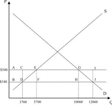
Figure 1: U.S. Steel Market After Dumping
The impact of the dumping on the U.S. can be further explored in Figure 1 above. This figure shows the U.S. market for steel goods and how it is impacted by the dumping country. The market price decreases from $540 to $340, since the U.S. goes from importing at the free market price to the lower export price of the foreign companies. That causes quantity demand to increase and quantity supply to decrease for the United States. Both consumer surplus and producer surplus are effected by this change in price due to dumping. Consumer surplus is defined by the area bounded by the demand curve on top and the market price on the bottom. Producer surplus is the area bounded by the market price on top and the supply curve on the bottom (Appleyard & Field, 2013). We see that consumer surplus increases by the area ABJG, while producer surplus decreases by the area ABDE. It makes sense that consumers would benefit since they can now purchase steel goods for a cheaper price, even if that price is artificially set. Producers would be hurt from the dumping since they are now competing against a cheaper product. Welfare loss from the dumping good can also be seen from the areas CDE and GJI. This represents the cost to society by the dumping of the steel goods. This provides another reason that the U.S. is
negatively impacted by the dumping countries.
To counteract the dumping from the foreign companies, the U.S. can implement a tariff to retaliate. In this case, the tariff would be an antidumping duty. The value of the duty would be equal to the dumping margin, so in this case it would equal 0.4138. In the equations from above, the tariff (𝑇) would be included in the equation for 𝑃,+ seen below
𝑃+, = 𝑃*(1 − 𝐷𝑀)(1 + 𝑇).
As stated above, 𝑇 = 𝐷𝑀 so that means that (1 − 𝐷𝑀)(1 + 𝑇) would approximately equal 1.
continue to be hurt by the losses of 20𝑃*∗ 𝐷𝑀, and that will continue in the long-run as long as
the tariff remains in place. Implementing an antidumping duty should effectively increase the price of steel from the named foreign companies and lead to a decrease in imports from those companies.
While these impacts of an antidumping duty are expected, there are other ways that trade could be impacted from the duty. Instead of the U.S. going back to buying steel from U.S. steel producers, trade could be diverted from the named countries to the non-named countries instead. That would leave U.S. firms back in the situation as when the named countries were dumping, since consumers start importing from non-named countries instead of going back to relying on U.S. firms for the steel goods. That is one of the main issues of antidumping duties explored in this paper and should be taken into consideration when a country implements an antidumping duty.
3. Literature Review
an international policy is imposed. The difference is that my paper focuses on antidumping duties impact on trade diversion instead of Free Trade Agreements.
My paper also contributes to literature that looks specifically at antidumping duties. Prusa (1996) looks at the effect of all U.S. antidumping duties (AD duty) from 1980 to 1988 on trade volume and trade diversion. He looks at the trade effect on named countries in the duties, as well as on non-named countries in order to show the level of trade diversion, which is the same method that is applied in this paper. The findings were that AD duties restricted the volume of trade for named countries, substantial trade diversion from named countries to non-named countries occurred, and AD petitions that were rejected still decreased imports from those named countries. While his study is fairly similar to this paper, there still are some key differences. This paper focuses only on one U.S. industry (steel), studies more recent AD duties (1990-2000), and uses more than just a year dummy variable to control for macroeconomic trends. By using more controls for macroeconomic trends, my paper helps control for potential bias from omitting key variables that impact U.S. imports (ex. U.S. production, foreign prices, exchange rate).
My paper also uses a model that will be different than these studies’ models. The key variables will be similar to previous papers, but this model will contain more control variables to minimize the omitted variable bias within the model. Previous models only include calendar dummies to control for macroeconomic trends, but this paper will include variables for foreign prices, U.S. production, foreign production, exchange rates, and then month and year dummies to control for seasonality. Looking at the steel industry and adjusting the model will help in further understanding antidumping duties and their impact on trade diversion.
4. Empirical Results I. Data
In order to examine the effects of antidumping duties on trade, panel trade data is constructed. First, the antidumping data is collected from the Global Antidumping Database (GAD) which is maintained by the World Bank (Data Catalog, n.d.). This dataset contains information on all the antidumping duties the U.S. has introduced from 1980 to 2015, including the country it was imposed on, the initiation date, and the actual size of the duty (as a
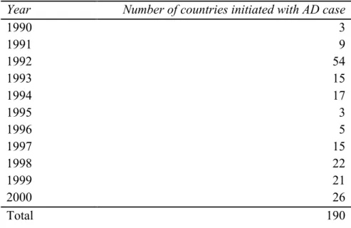
number of countries with firms that were initiated with an antidumping case per year. It shows that 1992 had the largest number of countries with initiated firms, while 1995 only had three.
Table 1: Most Frequently Named Countries, 1990-2000
Country Number of AD Cases
Japan 18
South Korea 16
Brazil 15
Taiwan 12
Germany 12
Canada 10
France 9
India 8
Table 2: Number of countries initiated with AD case per year
Year Number of countries initiated with AD case
1990 3
1991 9
1992 54
1993 15
1994 17
1995 3
1996 5
1997 15
1998 22
1999 21
2000 26
Total 190
product from all countries is collected within the time frame of 1989 to 2003 and are measured in quantity terms. It is also collected as monthly data, in order to see the immediate impact of the duties. One restriction made to the data is dropping countries when they only exported a certain steel product once during the entire 1989-2003 time period. After collecting both the import and AD data, the two datasets are merged and then grouped by country and product in order to create a panel dataset that does not have any duplicate observations.
The merged dataset is the what will be used in the regression. There are 180 months of data (1989-2003) for 37 categories of steel products. For each steel product, the quantity of imports is measured from each exporting country, which is about 50 exporters per steel product.
Within the dataset, named countries and non-named countries are categorized. To do this, a named dummy variable is created to represent which countries have a duty placed on them for a certain steel product at a certain time period. The named variable will equal 1 if a duty is initiated for a specific steel product from a country and it will remain equal to 1 until either the duty is not imposed or the duty was imposed but is no longer imposed. Figure 2 shows a timeline of the antidumping duties process.
In this timeline the time variable is t, which represents months. We see that in t=2 an antidumping case is opened up, which starts the investigation. The investigation continues until the ITC and ITA decide whether or not the duty should be imposed. Even if the duty is not
t=11
t=1 t=2 t=3 t=4 t=5 t=6 t=7 t=8 t=9 t=10 t=12 t=13 t=14 Initiation of
investigation
Duty Imposed
imposed, their can be an investigation effect, which means that by just starting an AD
investigation imports from the named countries decrease. In this case, the duty is imposed in t=4, so we see how imports change after initiation of an investigation in t=2 and we see how they change further once the duty is imposed in t=4. That duty continues to be imposed on those named companies until a time period when the duty is removed. This would be done if the named company stops dumping or if the U.S. decided it no longer needed the duty to be in place. In this example, the duty remains imposed until t=10. In regard to the named variable described above, this company/country would have a named variable equaling 1 from t=2 to t=10.
Otherwise, they are not considered named and the named variable equals 0.
The dependent variable within the dataset is quantity of steel imports, while two key independent variables are duty and an interaction between duty and a decision dummy. Going back to Figure 2, the duty variable will equal the percentage of the duty throughout the
antidumping process. There is a preliminary duty percentage announced once the investigation is initiated, but the duty percentage may change when it is decided to impose the duty. The decision dummy variable refers to that decision point on the timeline of whether or not to impose the duty. The decision dummy will equal 1 when a duty is levied and 0 if not. It will also remain 1 for all the months that the duty is imposed. By interacting the duty variable with the decision dummy variable, we are able to see how imports change when a duty is levied or not.
An issue arises when we focus on when countries are not being imposed with a duty. We want to see how these imports from non-named countries are affected when other named
Japanese firm was taxed 50% and the Spanish firm was taxed 20%). That made it difficult to know what the duty variable should be for the non-named countries of that antidumping duty. A way to represent the duty effect is calculating a weighted duty variable for the non-named countries. The calculation is:
𝑊𝑒𝑖𝑔ℎ𝑡𝑒𝑑𝐷𝑢𝑡𝑦Q,RS = bX8TRUV,WX ∗Z[\]^R_V,W`aX Z[\]^R_V,W`aX b
X
.
In this equation, 𝐷𝑢𝑡𝑦Q,RS represents the duty imposed on a country j for good i in time t. The
variable 𝐼𝑚𝑝𝑜𝑟𝑡𝑠Q,R&DS represents the imports of good i from a countries j (including both named
and non-named) in time t-1, which is the month prior to the initiation of the duty. The weighted duty equation shows that it is equal to the sum of the duty percentages for all the countries named for a specific antidumping duty, and then multiplied by the share of total U.S. imports coming from the named countries. Imports from the month prior to the initiation of the duty are used in order to have imports that are not already impacted by the initiation of the duty. This new weighted duty variable will be used to represent the trade diversion that occurs from imposing an antidumping duty. It shows how imports from non-named countries are impacted due to the creation of an antidumping duty.
A duty+ variable will also be created and interacted with the weighted duty variable. The duty+ variable will equal 1 whenever the variable duty is not equal to 0, and it will take the value of 0 otherwise. This variable is created and interacted with the weighted duty variable in order to prevent any confounding effects that result from including the weighted duty variable into the regression.
prices) are calculated by dividing the import values by the quantities. The producer price index for steel and iron U.S. commodities comes from the Federal Reserve Economic Data (Producer Price Index by Commodity for Metals and Metal Products: Iron and Steel (WPU101) | FRED |
St. Louis Fed, n.d.). A drawback of this index is that it includes more steel goods than those covered by the antidumping duties, but it still helps represent U.S. steel prices in the model. The exchange rate data is collected from the International Monetary Fund (Exchange Rate Archives by Month, n.d.). The exchange rate here is defined as the amount of foreign currency that can be purchased by one U.S. dollar. The foreign production of steel products (quantity produced in kilograms) is collected from Comtrade, which is made by the United Nations (Download trade data | UN Comtrade: International Trade Statistics, n.d.).
The inclusion of the foreign prices, U.S. prices and exchange rate are meant to represent the real exchange rate. Since we use a producer price index for U.S. steel commodities, this representation of the real exchange rate is not perfect. In order to improve this estimation, two new variables are created to be another representation of the real exchange rate. These variables are created by the ratios
i$^QjkVX i$^QjkV ∗
i$^QjkV (lmX∗$$Z).
In the first ratio, 𝐹𝑃𝑟𝑖𝑐𝑒QS is the foreign price of steel good i from country j, and 𝐹𝑃𝑟𝑖𝑐𝑒Q is the
the foreign price of steel good i across all countries. In the second ratio, 𝐸𝑅S is the exchange rate
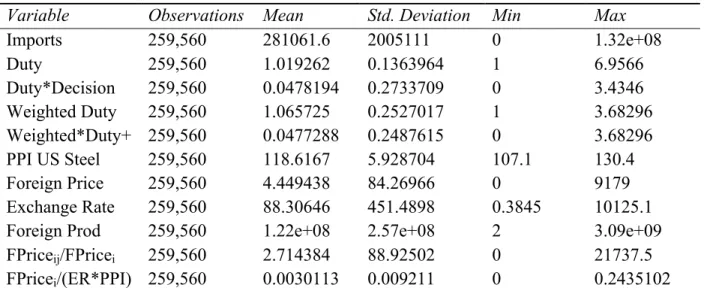
Table 3: Summary Statistics
Variable Observations Mean Std. Deviation Min Max
Imports 259,560 281061.6 2005111 0 1.32e+08
Duty 259,560 1.019262 0.1363964 1 6.9566
Duty*Decision 259,560 0.0478194 0.2733709 0 3.4346 Weighted Duty 259,560 1.065725 0.2527017 1 3.68296 Weighted*Duty+ 259,560 0.0477288 0.2487615 0 3.68296 PPI US Steel 259,560 118.6167 5.928704 107.1 130.4
Foreign Price 259,560 4.449438 84.26966 0 9179
Exchange Rate 259,560 88.30646 451.4898 0.3845 10125.1
Foreign Prod 259,560 1.22e+08 2.57e+08 2 3.09e+09
FPriceij/FPricei 259,560 2.714384 88.92502 0 21737.5 FPricei/(ER*PPI) 259,560 0.0030113 0.009211 0 0.2435102
Table 3 shows the summary statistics of the different variables, with the dependent and key variables at the top of the table. For the regression model, these variables will be converted to logarithmic form. This is done to respond to skews in the data towards large values. There are countries that the U.S. imports extremely large quantities of steel from, while other countries export much smaller quantities. Converting to logarithmic form will help reduce this skew in the data. One note about this conversion is that any imports that equal zero will be excluded from the regression. Taking the log of zero results in an undefined value, which means these observations are not included. Table 3 shows there are 259,560 observations of imports, but after converting to logarithmic form the number of observations drop to 64,045. This unfortunately is not quite as many observations as previously stated, but it still is a large enough sample size to derive
significant results.
II. Empirical Model
dependent variable and also uses a U.S. steel producer price index and unit values of foreign steel products to account for price, but the model adds other variables to control for different demand and supply shifters. The first model that is used in the regression is
𝑙𝑛𝐼𝑚𝑝𝑜𝑟𝑡𝑠Q,RS = 𝛽E+ 𝛽D𝑙𝑛𝐷𝑢𝑡𝑦Q,RS + 𝛽u 𝐷𝑒𝑐Q,RS ∗ 𝑙𝑛𝐷𝑢𝑡𝑦Q,RS + 𝛽v𝑙𝑛𝑃𝑃𝐼R+ 𝛽w𝑙𝑛𝐹𝑃𝑟𝑖𝑐𝑒Q,RS +
𝛽x𝑙𝑛𝐸𝑅RS+ 𝛽y𝑙𝑛𝐹𝑃𝑟𝑜𝑑Q,RS + 𝛽z𝑙𝑛𝐼𝑚𝑝𝑜𝑟𝑡𝑠Q,R&DS + 𝛽{𝑚𝑜𝑛𝑡ℎR+ 𝛽|𝑦𝑒𝑎𝑟R+ 𝛽DE𝑝𝑟𝑜𝑑𝑢𝑐𝑡R+ 𝜀Q,R.
The dependent variable 𝑙𝑛𝐼𝑚𝑝𝑜𝑟𝑡𝑠Q,RS is the quantity of U.S. imports of product i from all
countries j at time t (monthly). The variable 𝑙𝑛𝐷𝑢𝑡𝑦Q,RS denotes the size of the antidumping duty,
as a percentage. The next variable is an interaction between 𝐷𝑒𝑐Q,RS and 𝑙𝑛𝐷𝑢𝑡𝑦Q,RS. The variable
𝐷𝑒𝑐Q,RS is a decision dummy for each AD case and is equal to 1 when an AD proposal is affirmed
and remains 1 for all months where the duty is imposed. These two variables are the key variables of this model and represent the impact of an antidumping duty on U.S. imports from the named countries. Adding the interaction will show the effect of not just proposing a duty, but also if the duty is levied.
The next set of variables are control variables that are meant to decrease omitted variable bias by accounting for different macroeconomic factors that could affect U.S. imports of steel products. The first is 𝑙𝑛𝑃𝑃𝐼R, which is the producer price index for U.S. steel and represents the
U.S. price of steel. Foreign prices of steel are controlled for by the variable 𝑙𝑛𝐹𝑃𝑟𝑖𝑐𝑒Q,RS , which is
the unit values of each product from each country. The exchange rate with each country is
controlled for with 𝑙𝑛𝐸𝑅RS. The variable is 𝑙𝑛𝐹𝑃𝑟𝑜𝑑Q,RS , which is the foreign production of each
product i. This would control for an export-supply shifter. The variable 𝑙𝑛𝐼𝑚𝑝𝑜𝑟𝑡𝑠Q,R&DS is the
other things being equal. Lastly, the variables 𝑚𝑜𝑛𝑡ℎR and 𝑦𝑒𝑎𝑟R are month and year dummies
that will help control for seasonality and other macroeconomic trends and the variable 𝑝𝑟𝑜𝑑𝑢𝑐𝑡R
is a dummy that will control for the different steel products that that U.S. imports.
As stated previously, the model follows a similar format as the equations in section 2. By adding the different duty key variables and accounting for other variables that could impact imports, this model more accurately estimates the amount of steel imports into the United States after accounting for antidumping duties.
The next specification to this model would be changing the control variables to better represent the real exchange rate. This model would take away the separate variables of 𝑙𝑛𝑃𝑃𝐼R,
𝑙𝑛𝐹𝑃𝑟𝑖𝑐𝑒Q,RS , and 𝑙𝑛𝐸𝑅RS, and instead include the logarithms of the two ratio variables. Together,
these ratios will provide for a better understanding of the real exchange rate in the model. In order to calculate the amount of trade diversion that occurs from imposing
antidumping duties, another specification to the model is made. For this regression, the model is
𝑙𝑛𝐼𝑚𝑝𝑜𝑟𝑡𝑠Q,RS = 𝛽E+ 𝛽D𝑙𝑛𝐷𝑢𝑡𝑦Q,RS + 𝛽u 𝐷𝑒𝑐Q,RS ∗ 𝑙𝑛𝐷𝑢𝑡𝑦Q,RS + 𝛽v𝑙𝑛𝑊𝑒𝑖𝑔ℎ𝑡𝐷𝑢𝑡𝑦Q,RS +
𝛽w𝑙𝑛𝑊𝑒𝑖𝑔ℎ𝑡𝐷𝑢𝑡𝑦Q,RS ∗ 𝐷𝑢𝑡𝑦𝑃𝑙𝑢𝑠R+ 𝛽x𝑙𝑛𝑃𝑃𝐼R+ 𝛽y𝑙𝑛𝐹𝑃𝑟𝑖𝑐𝑒Q,RS + 𝛽z𝑙𝑛𝐸𝑅RS + 𝛽{𝑙𝑛𝐹𝑃𝑟𝑜𝑑Q,RS +
𝛽|𝑙𝑛𝐼𝑚𝑝𝑜𝑟𝑡𝑠Q,R&DS + 𝛽DE𝑚𝑜𝑛𝑡ℎR+ 𝛽DD𝑦𝑒𝑎𝑟R+ 𝛽Du𝑝𝑟𝑜𝑑𝑢𝑐𝑡R+ 𝜀Q,R.
The changes in this empirical model are the inclusion of 𝑙𝑛𝑊𝑒𝑖𝑔ℎ𝑡𝐷𝑢𝑡𝑦Q,RS and the interaction
between 𝑙𝑛𝑊𝑒𝑖𝑔ℎ𝑡𝐷𝑢𝑡𝑦Q,RS and 𝐷𝑢𝑡𝑦𝑃𝑙𝑢𝑠R. The calculation of the weighted duty was addressed
model. We attempt to control these confounding effects by adding in the interaction between weighted duty and duty+. The impact of the antidumping duty on the named countries can be seen by the three coefficients on the variables duty variable, the interaction between duty and decision, and the interaction between weighted duty and duty+. The remaining variables are the same as the first model.
One last specification is taking the third model and changing the variables that represent the real exchange rate. Just like the second specification, the two ratios will be included to have a better representation of the real exchange rate.
III. Results
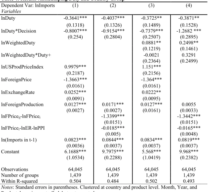
The first column of Table 4 shows the estimates for the first regression model. The results show that for a 1% change in Duty when a duty is initiated, imports from a named country
decrease by 0.36%. This represents an investigation effect, since even though the duty is not imposed there is still a decrease in imports. When the duty is imposed, imports from the named country decrease by an additional 0.8% for a 1% change in Duty. This also makes sense because the purpose of the duty is to reduce the amount of U.S. imports from these named counties. The fact that imports decrease by a larger percentage after imposing the duty shows how effective antidumping duties can be at reducing trade with dumping nations.
relationship with imports, which means that the U.S. imports more as the dollar gets stronger. This does make sense, since a stronger dollar makes imports cheaper, thus increasing imports.
The second column displays the regression results for the second specification of the model. This model contains the two ratios that make up the real exchange rate instead of
including those variables independently. These results show a 1% increase in Duty when a duty is initiated leads to a 0.4% decrease in U.S. steel imports from a named country. Imposing the duty leads to an additional 0.915% decrease for a 1% increase in Duty. The investigation effect seems to be similar as the previous specification, but the additional decrease in U.S. steel imports after imposing a duty is even larger than the results from the previous model. This again shows the strong impact against dumping countries when an antidumping duty is imposed. Going back to the example in section 2, we saw that dumping countries take a loss once they begin to dump. If nothing stops them from dumping, then in the long run they will obtain more market share and be able to offset those losses. Imposing an AD duty on the dumping country means that the dumping country will continue to take losses as long as they have an artificially lower price.
The third column shows the results for the regression model with weighted duty and the interaction between weighted duty and duty+. The amount of trade diversion that occurs when an antidumping duty is placed on a country is represented in the coefficient for weighted duty. The results show that for a 1% increase in weighted duty, U.S. steel imports from one non-named country increase by 0.088%. This shows that there is trade diversion from imposing an AD duty on a named country. The impact on U.S. steel imports from a named country is represented by the coefficients for duty, duty and decision interaction, and weighted duty and duty+ interaction. The signs are negative for both duty and the interaction between duty and decision, but the sign for the interaction between weighted duty and duty+ is positive, although the value is almost zero. This again shows the decrease in steel imports from these named countries. The controls also continue to display the correct sign.
These results show that imports from a named country will decrease after implementing an AD Duty, while imports from a non-named country will increase. Each coefficient, though, is in regard to just one named country or one non-named country. Due to this, the amount of trade diversion or destruction is difficult to comprehend. In order to provide a better picture of the extent of trade destruction/diversion, a simulation example was created.
Table 4: Results-Antidumping Duty and Country Group Dependent Var: lnImports
Variables
(1) (2) (3) (4)
lnDuty -0.3641*** -0.4037*** -0.3725** -0.3871**
(0.1318) (0.1326) (0.1489) (0.1528) lnDuty*Decision -0.8007*** -0.9154*** -0.7379*** -1.2682 ***
(0.254) (0.2804) (0.2507) (0.2895)
lnWeightedDuty 0.0881** 0.2498**
(0.1219) (0.1461)
lnWeightedDuty*Duty+ -0.0021 0.3291
(0.2364) (0.2499)
lnUSProdPriceIndex 0.9979*** 1.151***
(0.2187) (0.2156)
lnForeignPrice -1.3663*** -1.364***
(0.0161) (0.0161)
lnExchangeRate 0.0252*** 0.0222**
(0.0091) (0.0095)
lnForeignProduction 0.0127*** 0.0171*** 0.0127*** 0.0055 (0.0027) (0.0027) (0.0161) (0.0033)
lnFPriceij-lnFPricei -1.3399*** -1.3442***
(0.0151) (0.0151)
lnFPricei-lnER-lnPPI -0.0185*** -0.0165***
(0.005) (0.0048)
ln(Imports in t-1) 0.0823*** 0.0844*** 0.0834*** 0.0819*** (0.0036) (0.0037) (0.0037) (0.0037)
Constant 6.1688*** 9.7975*** 5.568*** 9.968***
(1.0534) (0.2288) (1.0419) (0.2382)
Observations 64,045 64,045 64,045 64,045
Number of groups 1,439 1,439 1,439 1,439
Within R-squared 0.504 0.484 0.502 0.493
Notes: Standard errors in parentheses. Clustered at country and product level. Month, Year, and Product dummies controlled, but not reported.
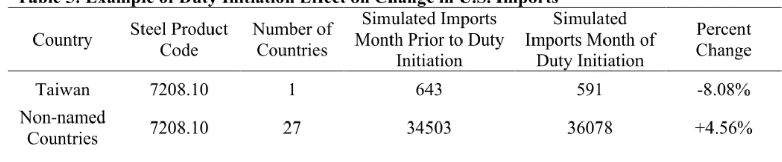
The simulation looks at one antidumping duty on Taiwan for a specific steel product category (7208.10). The first part of the simulation focuses on Taiwan and the change in U.S. imports from them from the month prior to the duty being initiated and the month the duty is initiated. The coefficients from Table 4 column 1 are multiplied by the values of those variables for Taiwan in both of these months. For each month, the multiplied values are summed together to get the predicted value for the logarithm of U.S. imports. The exponent of that predicted value is taken in order to get the simulated amount of U.S. imports for each month. Those simulated values are shown in Table 5. The percentage change in simulated imports in the month prior to initiation and the month of initiation is calculated and reported as a decrease by 8.08%. That shows the trade destruction that occurs after initiated the AD duty on Taiwan.
The next part of the simulation focuses on all 27 non-named countries for this particular AD duty. The coefficients from column 3 of Table 4 are used in this simulation since it includes the weighted duty variable. Each separate countries variable values for the two month periods are multiplied by the corresponding coefficient. These multiplied values are summed for each
separate country and then exponent for each of those summed values is taken. Then the exponent value for each named country is summed together to get the simulated imports for all non-named countries in each respective month. Those values are presented in Table 5 as well. The percentage change in simulated imports for non-named countries in the month prior to initiation and month of initiation is shown to be an increase of 4.56%.
Table 5: Example of Duty Initiation Effect on Change in U.S. Imports Country Steel Product Code Number of Countries
Simulated Imports Month Prior to Duty
Initiation
Simulated Imports Month of
Duty Initiation
Percent Change
Taiwan 7208.10 1 643 591 -8.08%
Through this simulation example, we see that imports from the named country do decrease after initiating a duty. We also see the total amount of trade diversion, instead of changes in imports from just one non-named country. The simulation shows an increase in imports from non-named countries by 4.56% once the duty is initiated. This provides a better picture of how imports from all non-named countries of a specific duty change.
One more step that is taken is running the regression solely on Taiwan for this steel product code. After running the regression, the regression’s coefficients are used in the same way as the previous simulation. This is done to test the robustness of the simulation and regression. Table 6 shows the simulated imports from Taiwan for both months after using these new coefficients.
The robustness check simulation also shows a decrease in U.S. imports from Taiwan. Table 6 shows that once the duty is initiated, imports decrease by 3.13%. This is less than what we saw in the previous simulation, but it is still showing the trade destruction effect that we were expecting would happen.
5. Conclusion and Extensions
The evidence presented in this paper shows how retaliatory tariffs can impact trade patterns differently based on whether or not a country is initiated/imposed with an antidumping duty. The imports from named countries are negatively effected by initiation of the retaliatory Table 6: Robustness Check Example of Duty Initiation Effect on Change in U.S. Imports
Country Steel Product Code Simulated Imports Month Prior to Duty Initiation Month of Duty Initiation Simulated Imports Percent Change
tariffs and then decrease even further once the tariff is imposed, which is one of the goals of these tariffs. Trade diversion was also shown to take place, since imports from non-named countries increase once a duty is initiated/imposed. Malhotra, Rus, and Kassam (2008) found no significant amount of trade diversion in the U.S. agriculture sector when imposing antidumping duties, so the steel industry may have a higher elasticity of substitution than the agriculture industry, which allows for more trade diversion to take place.
These results may also be applicable to President Trump’s retaliatory tariffs. Those tariffs may have the intended impact on U.S. imports from named countries, which would help fight against foreign companies that are dumping. What needs to be taken into account, though, is the trade diversion from the retaliatory tariffs. The evidence presented in this paper shows that trade diversion does take place and that will leave U.S. firms in a not as favorable position as intended. Policy makers must understand that antidumping duties and other retaliatory tariffs can be
effective at reducing named country imports, but other consequences can take place that reduce the effectiveness of these tariffs.
There are some extensions of this paper that could be explored further in future studies. Studies could focus on the countries/companies that are most commonly imposed with
Lastly, there is the idea of a domino effect for U.S. imports related to expectations. If U.S. importers can have some type of expectation of which foreign companies/countries will be imposed with a duty in the near future, then it is possible that their import decisions could be impacted by those expectations. They may not import from a relatively cheap foreign exporter since they believe that it will be imposed with an antidumping duty soon, and instead they will import from another more expensive exporter that is not at risk of being imposed with an
Work Cited
| Data Catalog. (n.d.). Retrieved November 18, 2019, from
https://datacatalog.worldbank.org/dataset/temporary-trade-barriers-database-including-global-antidumping-database/resource/dc7b361e
Bartholomew, B. (2019). The Steel Industry and its Place in the American Economy. BDO USA.
https://www.bdo.com/insights/business-financial-advisory/valuation-business-analytics/the-steel-industry-and-its-place-in-the-american-e
Berry, S., Levinsohn, J., & Pakes, A. (1995). Voluntary Export Restraints on Automobiles: Evaluating a Strategic TradePolicy (Working Paper No. 5235). National Bureau of Economic Research. https://doi.org/10.3386/w5235
Data Request | DataWeb. (n.d.). Retrieved November 18, 2019, from https://dataweb.usitc.gov/trade/search/Import/HTS
Download trade data | UN Comtrade: International Trade Statistics. (n.d.). Retrieved November 13, 2019, from https://comtrade.un.org/data/
Exchange Rate Archives by Month. (n.d.). Retrieved November 13, 2019, from https://www.imf.org/external/np/fin/data/param_rms_mth.aspx
Irwin, D. A. (n.d.-a). Clashing over Commerce: A History of US Trade Policy. 41. Irwin, D. A. (n.d.-b). Clashing over Commerce: A History of US Trade Policy. 43. Irwin, D. A. (n.d.-c). Clashing over Commerce: A History of US Trade Policy. 41.
Producer Price Index by Commodity for Metals and Metal Products: Iron and Steel (WPU101) |
FRED | St. Louis Fed. (n.d.). Retrieved February 28, 2020, from https://fred.stlouisfed.org/series/WPU101
Prusa, T. J. (1996). The Trade Effects of U.S. Antidumping Actions (Working Paper No. 5440). National Bureau of Economic Research. https://doi.org/10.3386/w5440
Russ, K. N., & Swenson, D. L. (2019). Trade Diversion and Trade Deficits: The Case of the Korea-U.S. Free Trade Agreement. Journal of the Japanese and International Economies, 52, 22-31.
Understanding Antidumping & Countervailing Duty Investigations | USITC. (n.d.). Retrieved November 18, 2019, from https://www.usitc.gov/press_room/usad.htm