Hyun_unc_0153D_14679.pdf

ANALYSIS OF INTERVAL CENSORED DATA USING A

LONGITUDINAL BIOMARKER

Noorie Hyun

A dissertation submitted to the faculty of the University of North Carolina at Chapel

Hill in partial fulfillment of the requirements for the degree of Doctor of Philosophy in

the Department of Biostatistics in the Gillings School of Global Public Health.

Chapel Hill

2014

Approved by:

Dr. Donglin Zeng

Dr. David J. Couper

Dr. Jianwen Cai

c

○ 2014

Noorie Hyun

ABSTRACT

NOORIE HYUN: Analysis of Interval Censored Data Using a

Longitudinal Biomarker

(Under the direction of Dr. Donglin Zeng and Dr. David J. Couper)

In many medical studies, interest focuses on studying the effects of potential risk

factors on some disease events, where the occurrence time of disease events may be

defined in terms of the behavior of a biomarker. For example, in diabetic studies,

diabetes is defined in terms of fasting plasma glucose being 126

mg

/

dl

or higher. In

practice, several issues complicate determining the exact time-to-disease occurrence.

First, due to discrete study follow-up times, the exact time when a biomarker crosses

a given threshold is unobservable, yielding so-called interval censored events. Second,

most biomarker values are subject to measurement error due to imperfect technologies,

so the observed biomarker values may not reflect the actual underlying biomarker levels.

Third, using a common threshold for defining a disease event may not be appropriate

due to patient heterogeneity. Finally, informative diagnosis and subsequent treatment

outside of observational studies may alter observations after the diagnosis. It is well

known that the complete case analysis excluding the externally diagnosed subjects can

be biased when diagnosis does not occur completely at random.

defined for any given threshold value. Second, we extend the marginal likelihood to a

pseudo-likelihood by multiplying the likelihoods over all observation times. Finally, to

adjust for externally diagnosed cases, we consider a weighted pseudo-likelihood

estima-tor by incorporating inverse probability weights into the pseudo-likelihood by assuming

that external diagnosis depends on observed data rather than unobserved data. We

estimate the three model parameters using the nonparametric EM, pseudo-EM and

weighted-pseudo-EM algorithm, respectively.

ACKNOWLEDGMENTS

I am extremely grateful to my advisors, Drs. Donglin Zeng and David J. Couper

for their thoughtful guidance, insightful advice, and sincere encouragement during my

dissertation research period. I know I would not be able to reach the end of this long

journey without their help. The hands-on experience under supervision of my advisors

have made me more confident as a researcher. I would also like to thank Drs. Donglin

Zeng and David J. Couper for their financial support as well.

I would like to express my sincere gratitude to my committee members,Drs. Jianwen

Cai, Michael G. Hudgens, and M. Alan Brookhart for their constructive and perceptive

comments on my dissertation papers.

TABLE OF CONTENTS

LIST OF TABLES

. . . ix

LIST OF FIGURES

. . . x

1 INTRODUCTION

. . . .

1

2 Literature Review . . . .

5

2.1 Interval Censored Data . . . 6

2.1.1 Current Status Data . . . 6

2.1.2 Case 2 Interval Censored Data . . . 14

2.1.3 Panel Count Data . . . 19

2.1.4 Mixed Case of Interval Censored Data . . . 23

2.2 Measurement Error in Data . . . 26

2.2.1 Linear Regression with Response Error . . . 28

2.2.2 Logistic Regression with Response Error . . . 29

2.2.3 Semiparametric Methods for Validation Data . . . 30

2.3 Weighted Estimating Equations Accounting for

MAR Data . . . 31

3 Threshold-Dependent Proportional Hazards Model

for Analyzing Time-to-Event Defined by Biomarker

with Subject to Measurement Error . . . 35

3.1 Introduction . . . 35

3.2 The ARIC Study . . . 38

3.3.1 Model . . . 39

3.3.2 Inference Procedure . . . 42

3.3.3 Variance Estimation . . . 44

3.4 Asymptotic Results . . . 45

3.5 Simulation Study . . . 48

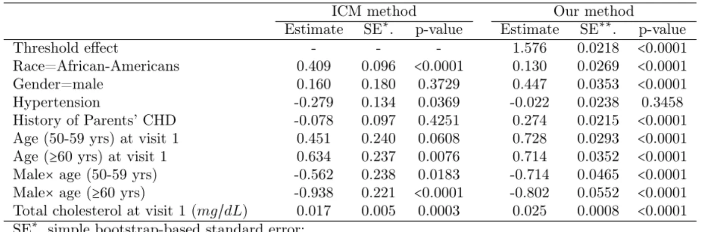
3.6 Analysis of the ARIC Study Data . . . 50

3.7 Concluding Remarks . . . 53

4 Semiparametric Regression Model for

Analyz-ing Time-to-Event Defined by Extreme

Longi-tudinal Biomarkers . . . 60

4.1 Introduction . . . 60

4.2 Method . . . 62

4.2.1 Model . . . 62

4.2.2 Inference Procedure . . . 64

4.2.3 Variance Estimation . . . 65

4.3 Asymptotic Results . . . 69

4.4 Simulation Study . . . 71

4.5 Application . . . 74

4.6 Concluding Remarks . . . 76

5 Weighted Pseudo-Likelihood for Adjusting

In-formative Diagnosis: an Application to

Time-to-Hypercholesterolemia in the ARIC study . . . 81

5.1 Introduction . . . 81

5.2 Method . . . 83

5.2.1 Weighted Pseudo-Likelihood . . . 83

5.2.2 Inference Procedure . . . 85

5.3 Asymptotic Results . . . 89

5.4 Simulation Study . . . 92

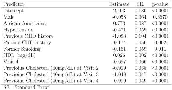
5.5 Application . . . 94

5.6 Concluding Remarks . . . 97

6 Summary and Future Work . . . 101

Appendix A: Technical Details for Chapter

3

. . . 104

A.1 Identifiability and Derivation of Efficient Score Functions . . . 104

A.2 Proof of Asymptotic Results . . . 108

Appendix B: Technical Details for Chapter

4

. . . 119

B.1 Identifiability and Derivation of Pseudo-Efficient

Score Functions . . . 119

B.2 Proof of Asymptotic Results . . . 121

Appendix C: Technical Details for Chapter

5

. . . 133

C.1 Proof of Asymptotic Results . . . 133

LIST OF TABLES

3.1 Baseline Characteristics of the Study Participants . . . 57

3.2 Simulation Result in the Scenario with

Contin-uous Random Time Points . . . 58

3.3 Analysis of Time to Diabetes Occurrence from

the ARIC Study Data . . . 59

4.1 Simulation Result . . . 79

4.2 Application to the ARIC Study Data . . . 80

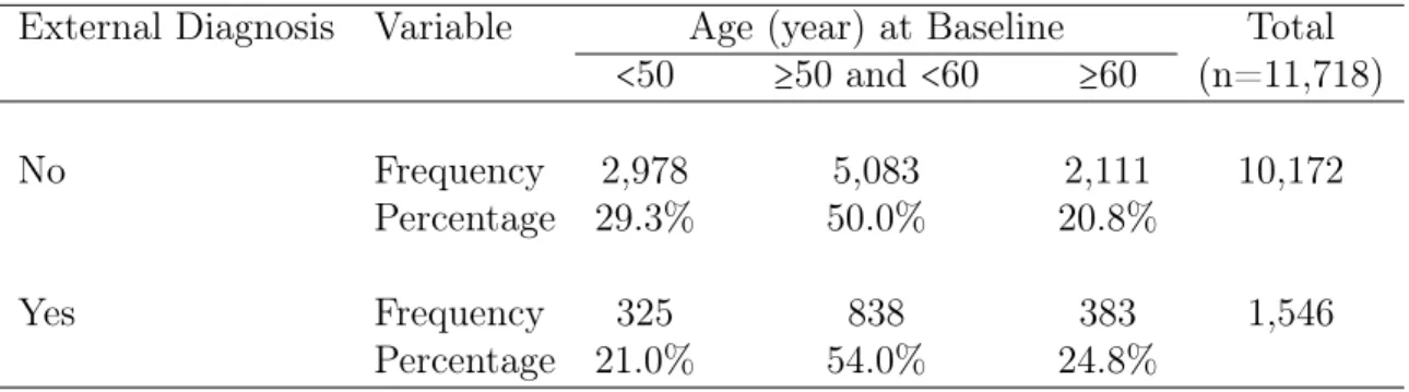
5.1 Prevalence of Externally Diagnosed Hypercholesterolemia . . . 98

5.2 Simulation Result When Missing Rate is 13% . . . 99

5.3 Logistic Regression for the Probability of No

Ex-ternal Diagnosis as Hypercholesterolemia . . . 99

5.4 Application to the ARIC Study Data . . . 100

LIST OF FIGURES

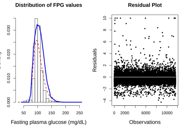
3.1 Distribution of Fasting Blood Glucose Values . . . 55

3.2 Quantile-Quantile and Residual Plots . . . 56

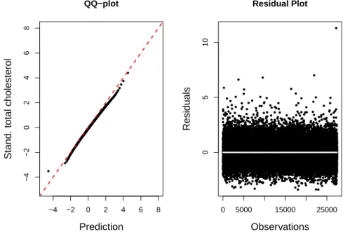
4.1 Quantile-Quantile and Residual Plots . . . 78

5.1 Mean Trend of Total Cholesterol Levels in

CHAPTER1: INTRODUCTION

Many longitudinal studies of chronic disease such as cancer, AIDS, and diabetes

monitor patients for biomarkers, as an indicator of disease occurrence, in order to

investigate potential associations between risk exposures and time to disease occurrence.

For disease events determined by some biomarker and threshold, when interval between

visits is long or patients miss visits, the exact date of the event that an individual’s

biomarker value crosses the threshold is unobservable. Instead, what is usually known

are the latest and earliest visit dates at which an individual’s biomarker value crosses

a given threshold. Such data is called interval censored data. Using the interval rather

than the exact date of event occurrence may lead to invalid inferences (Lindsey and

Ryan 1998).

Most biomarkers measurement has variation and the variation consists of short-term

intra-individual variability and measurement error. Assay variability and within-person

effects complicate determination of whether an individual’s biomarker has actually

exceeded the threshold. In clinical practice,

ad hoc

approaches that are used to take

into account biomarker variability include taking two or more measurements over a

period of time. Regarding measurement error, for example, the National Institute of

Standards and Technology maintains the blood sample materials as the gold standard

and provides guidelines for instrument manufactures to determine the accuracy of their

measurement devices. If measurement error is non-ignorable but ignored in the analysis,

the analysis may yield an inaccurate conclusion.

threshold that are usually ignored in practice. The threshold is generally regarded

as a fixed constant that is appropriate for everyone; however, this may not be

appropri-ate to all biomarkers. For instance, hypercholesterolemia does not cause symptoms but

can significantly increase risk of developing coronary heart disease (CHD). To reduce

risk, including that of CHD, people with substantially elevated cholesterol levels are

advised to start therapeutic lifestyle changes or drug therapy. The cholesterol level at

which to consider therapeutic intervention varies across different risk categories such

as smoking, hypertension, age, etc. (the National Cholesterol Education Program

Ex-pert Panel 2001)

Finally, informative diagnosis outside of observational studies, which causes alter

observations after the diagnosis. It is well known that the complete case analysis

excluding the externally diagnosed subjects can be biased when diagnosis does not

occur completely at random (Ibrahim et al. 2005).

We are motivated by the Atherosclerosis Risk in Communities (ARIC) study and

an ancillary ARIC study, which present the problems described above. The ARIC

Study recruited a population-based cohort from four U.S. communities, namely, Forsyth

County, NC, Jackson, MS, suburbs of Minneapolis, MN, and Washington County, MD.

Participants underwent a baseline examination in 1987-1989 had three follow-up

exam-inations at approximately three-year intervals, and a further examination in 2011-2013.

The ARIC Study was designed to investigate the causes of atherosclerosis, and

hyper-cholesterolemia is a crucial risk factor for atherosclerosis. Hence, assessing risk factors

associated with time-to-hypercholesterolemia is of interest. An ancillary study of the

ARIC study investigated type 2 diabetes mellitus The standard ARIC definition of

diabetes is having a fasting plasma glucose (FPG)

≥

126

mg

/

dL

, non-fasting glucose

≥

200

mg

/

dL

, a self-reported physician diagnosis of diabetes, or use of diabetes medication

time-to-disease occurrence, diabetes or hypercholesterolemia, and in the dissertation,

we focus on the time until the biomarkers reach the corresponding threshold levels.

To resolve these four issues, we consider a semiparametric model for analyzing

threshold-dependent time-to-event defined by extreme-value-distributed and

longitudi-nal biomarkers and break down the problems into the three steps:

(1)

Threshold-Dependent Proportional Hazards Model for Analyzing Time-to-Event

Defined by Biomarker with Subject to Measurement Error

: to mitigate the

prob-lems, we concentrate on the first follow-up visit after baseline and ignore the

infor-mative external diagnosis altogether. We propose a semiparametric model based

on a generalized extreme value distribution for the time-to-disease occurrence.

By assuming the latent error-free biomarkers to be non-decreasing, the proposed

model has a natural class of proportional hazards models for the time-to-event

defined for any given threshold value. To account for the additive measurement

errors, we estimate the model parameters using the nonparametric maximum

likelihood approach.

(2)

Semiparametric Regression Model for Analyzing Time-to-Event Defined by

Ex-treme Longitudinal Biomarkers

: the model proposed in the first step is extended

to model the longitudinal biomarkers at follow-ups by constructing a

pseudo-likelihood, which is multiplying the marginal likelihoods at follow-ups.

than unobserved data. We employ a marginal structure model based on

auxil-iary information and subject’s status at the previous visits to predict an external

diagnosis.

We estimate the three model parameters via the nonparametric Expectation

Maxi-mization (EM), pseudo-EM, and weighted-pseudo-EM algorithm, respectively. In this

dissertation, we theoretically investigate the models and estimation methods. We

pro-vide a series of simulations, to examine each model and estimation method comparing

them with the existing methods. Consistency, convergence rates, and asymptotic

dis-tribution of estimators are investigated using the empirical process techniques. We

illustrate the first marginal model by applying it to data from the diabetes ancillary

ARIC study and the other two models by applying those to data from the ARIC study.

In Chapter

2

, existing methods to address each problem, interval censored data,

CHAPTER2: LITERATURE REVIEW

Interval censoring in survival analysis is a generalized scheme of left or right

censor-ing. Observed exact failure times practically correspond to narrow intervals (Turnbull

1976, Kalbfleisch and Prentice 2002). In left or right censoring, the probability that

exact failure time is observed is positive; however, we are unable to observe it at all in

interval censored data. Therefore, statistical methods and inferences for interval

cen-sored data are more complicated than left or right cencen-sored data (Huang and Wellner

1997).

2.1

Interval Censored Data

2.1.1

Current Status Data

When only one observation time is applied and each patient is known to experience

the onset of the event either before or after the observation time, the data are called as

case 1

interval censored data or

current status data

. Current status data often occur

in cross-sectional studies when the outcome is a mile-stone event such as the onset of

chronic disease. Also, current status data are easily found in animal studies such as

tumorigenicity experiments on nonlethal tumors (Hoel and Walburg 1991).

For the subject

i

with a vector of covariates

X

, let

T

be the unobservable failure

time and

V

be the examination or observation time. Then the observed data of the

subject

i

are

(

V

, δ

,

X

)

denote as

W

, where

δ

=

I

(

T

≤

V

)

. It is assumed that

T

is independent of

V

given

X

. In addition, the joint distribution of

(

V,

X

)

is assumed

to be independent on

θ

-that is a vector of coefficients for the covariate

X

-and any

unspecified non-decreasing baseline function of

T

.

Survival Estimation with Current Status Data

In this section, nonparametric maximum likelihood estimators (NPMLEs) for the

survival or distribution function of current status data are reviewed. Denote the ordered

observed times by

{

V

∣

i

=

1

, . . . , n

}

, that is,

V

≤

V

for

i

=

1

, . . . , n

−

1

.

The observed log likelihood function for current status data

{(

V

, δ

)∣

i

=

1

, . . . , n

}

is

l

(

F

) =

n

∑

i=1

{

δ

log

F

(

V

) + (

1

−

δ

)

log

(

1

−

F

(

V

))}

,

(2.1)

where

F

(⋅)

is the distribution function of

T

.

minimizing

n

∑

i=1

n

[

δ

n

−

F

(

V(

)]

2

,

subject to

F

(

V(

) ≤

. . .

≤

F

(

V(

)

,

(2.2)

where

n

=

n

and

n

=

n

−

i

+

1

(Robertson et al. 1988). The NPMLE for

F

are determined

only at the observation times

{

V

}

with

δ

=

1

,

1

≤

i

≤

n

. Let

{

s

}

=1

be the uniquely

ordered observation times at which

δ

=

1

for

1

≤

i

≤

n

. The set of values of

{

F

(

s

)}

=1

that minimizes (

2

.

2

) is referred to as the isotonic regression of

{

1

/

n

, . . . ,

1

/

n

}

with

weights

{

n

, . . . , n

}

We can find a NPMLE for

F

minimizing (

2

.

2

) by various approaches. Using the

max-min formula for isotonic regression, Ayer et al. (1955) obtained the explicit forms

for

{

F

ˆ

(

s

)}

as

ˆ

F

(

s

) =

max

u≤j

min

∑

δ

v

−

u

+

1

.

(2.3)

They also introduced the pool adjacent violators algorithm (PAVA) and recommended

this algorithm rather than direct calculation of the formula in (

2

.

3

) to facilitate the

computation.

Huang and Wellner (1997) proposed an algorithm: after plotting

(

i,

∑

δ(

)

, i

=

1

, . . . , n

and forming the Greatest Convex Minorant (GCM),

G

of the points in the

plot, then left-derivative of

G

at

_i

is calculated for

_F

ˆ

n

(

V(

)

,

i

=

1

, . . . , n

. This algorithm

obtains the same NPMLE as the max-min formula in

(

2

.

3

)

. The GCM algorithm is

faster than the PAVA algorithm from a small to a large sample size except when the

left truncation probability is over 0.85 (Zhang and Newton 1997).

Regression Model with Current Status Data

Regression analysis of survival data is used to quantify the effect of some covariates

on the survival time or to predict the survival probabilities for new individuals. In this

section, we review commonly used regression models for current status data such as

the Cox proportional hazards (PH) models, proportional odds models, additive hazard

models, and accelerated failure time (AFT) models, etc.

The observed log likelihood for current status data is given by

l

(

F

∣

W

) =

n

∑

i=1

{

δ

log

F

(

V

∣

W

) + (

1

−

δ

)

log

(

1

−

F

(

V

∣

W

))}

,

(2.4)

where

F

(

t

∣

W

)

is the distribution function of

T

given the observed data.

Current status data almost allows us to obtain explicit forms of the efficient influence

function and semiparametric efficient variance for regression parameters.

Each regression model is the special case of the following transformation model. The

transformation model postulates that the conditional distribution

F

(

t

∣

x

)

of

T

given the

covariates

X

=

x

satisfies

g

(

F

(

t

∣

x

)) =

h

(

t

) +

θ

x,

(2.5)

where

g

is a specified function;

h

(

t

)

is an unknown non-decreasing function;

θ

is the

unknown finite d-dimensional regression parameter.

First, if we take

g

(

s

) =

log

[−

log

(

1

−

s

)]

,

0

<

s

<

1

, then (

2

.

5

) results in the

propor-tional hazards model by Cox (1972). The Cox proporpropor-tional hazards model has been

the most commonly used for survival analysis due to the availability of efficient

infer-ence procedures that are implemented in all statistical software packages. The model

postulates

λ

(

t

∣

X

=

x

) =

λ

(

t

)

e

T_x

for the hazard function of the survival time

T

given the covariate

x

, where

λ

(

t

)

denotes

an unknown baseline hazard function. The regression parameter of

θ

provides the log

hazard ratio of

x

on time to the event. Between two levels of the covariate

X

, the PH

model constrains the ratio of the hazards to be constant over time. The model in (

2

.

6

)

can be cast as a transformed linear model of

log

´

λ

(

u

)

du

=

−

θ

X

+

, where

follows

the extreme value distribution of

1

−

exp

(−

e

)

(Dabrowska and Doksum 1988).

The observed log likelihood under the model in

(

2

.

6

)

is

l

(

θ,

Λ

∣

W

) =

n

∑

i=1

{

δ

log

[

1

−

exp

(−

Λ

(

V

)

exp

(

θ

X

)) ] − (

1

−

δ

)

exp

(

θ

X

)

Λ

(

V

)}

,

where

Λ

(

t

) =

´

0

λ

(

u

)

du

.

Related to PH regression models for current status data, Huang (1996) provided very

influential and thorough study. He obtained a maximum profile likelihood estimator

(profile-MLE) for

(

θ,

Λ

)

by the iterative convex minorant algorithm (this algorithm

will be reviewed in detail in section

2

.

1

.

2

). The consistency, asymptotic normality, and

semiparametric efficiency of the profile-MLE for regression parameters were established

under certain regularity conditions. The convergence rate of the estimators

_Λ

̂

dominates

the convergence rate of (

_θ,

̂

_Λ

̂

) by

_n

. Nonetheless, it was shown that the regression

parameter estimates asymptotically converges to normal distribution in the rate of

√

n

. The profile likelihood method requires intensive computation for data with large

covariates.

Second, if we take

g

(

s

) =

logit

(

s

) ≡

log

[

s

/(

1

−

s

)]

for

0

<

s

<

1

in the regression

model of (

2

.

5

), then we obtain a proportional odds regression model:

logit

[

F

(

t

∣

X

=

x

)] =

h

(

t

) +

θ

x.

(2.7)

is the log odds ratio for two samples with unit difference in the

k

th covariate. In

the proportional odds model, the hazard ratio for two samples is not constant over

time but converges to unity as time

t

increases. The model (

2

.

7

) can be described

as a transformed linear model of

h

(

t

)

=

θ

X

+

, where

has the logistic distribution

of

[

1

+

exp

(−

)]

(Dabrowska and Doksum 1988). For right censored data, Bennett

(1983a;b) provided a proportional odds model and a log-logistic regression model.

Pet-titt (1984) suggested several levels of specification about

h

(

t

)

in the proportional odds

model (

2

.

7

).

The observed log likelihood function under the model (

2

.

7

) is

l

(

θ, h

∣

W

) =

n

∑

i=1

δ

{

h

(

V

) +

θ

X

} −

log

[

1

+

exp

{

h

(

V

) +

θ

X

} ]

.

(2.8)

Rossini and Tsiatis (1996) suggested a semiparametric proportional odds model for

current status data using an approximate maximum likelihood. The approximate

like-lihood is replacing

h

(

t

)

in the likelihood (

2

.

8

) with a non-decreasing step function. The

maximum likelihood estimator (MLE) maximizing the approximate likelihood can be

viewed as a sieve MLE based on the sieve of non-decreasing continuous piecewise

con-stant functions. They showed consistency, asymptotic normality, and semiparametric

efficiency of the regression parameters estimates under certain regularity conditions and

provided the explicit form of the asymptotic variance for the estimates.

Third, we consider an accelerated failure time model:

log

(

T

) =

θ

X

+

,

(2.9)

model can be written as

F

{

log

(

T

)∣

X

} =

F

{

log

(

T

) −

θ

X

}

in terms of a conditional

distribution.

The observed log likelihood under the model (

2

.

9

) is

l

(

F

∣

W

) =

n

∑

i=1

[

δ

log

F

(

log

V

−

θ

X

) + (

1

−

δ

)

log

{

1

−

F

(

log

V

−

θ

X

)} ]

.

(2.10)

Huang and Wellner (1997) proposed a profile-MLE under the AFT model. They

showed consistency of the profile-MLE and provided the information bound for

θ

under

certain regularity conditions; however, left an open problem about the convergence rate

of

_θ

̂

. The estimated MLE of

_F

_(⋅∣

_θ

₎

for each fixed

_θ

is not smooth, and it results in the

non-smooth profile likelihood with respect to

θ

, so the convergence rate is unspecified

yet.

Tian and Cai (2006) constructed an estimator under the AFT model by inverting a

Wald-type statistics for testing a null proportional hazards. Due to the equivalence

be-tween two assumptions: residual in

(

2

.

9

)

is independent of

X

;

S

(

t

∣

X

) =

S

(

t

)

,

the regression parameters can be estimated by solving the estimating equation,

γ

̂

(

θ

) =

o

(

n

)

, where

̂

γ

is the NPMLE of Huang (1996). Using the semiparametric efficient

variance of

γ

,

B

calculated by Huang (1996), the asymptotic variance of

_θ

̂

can be

approximated by sandwich variance,

D

_B

(

D

)

, where

D

=

dγ

(

θ

)/

dθ

∣

. The

estimator was proved to be consistent under certain regularity conditions.

Finally, if we take

g

(

s

) = −

log

(

1

−

s

)

,

0

<

s

<

1

, in the regression model of (

2

.

5

),

then we have an additive hazard regression model:

λ

(

t

∣

X

=

x

) =

λ

(

t

) +

θ

x

(

t

)

,

(2.11)

where

λ

(

t

)

is an unspecified baseline hazard function. This model describes the

Lin et al. (1998) proposed an additive hazard model based on a counting process

and martingale theory for current status data. When the counting process is defined

as

N

(

t

) = (

1

−

δ

)

I

(

V

≤

t

)

, which jumps by unit whenever the subject

i

is observed at

time t and found still to be failure-free, the probability that the counting process has

one is: under the assumption that

T

and

V

are independent

dH

(

t

) =

e

T_X∗

(t)

dH

(

t

)

,

(2.12)

where

dH

(

t

) =

e

_d

_Λ

V

(

t

)

and

X

(

t

) =

´

0

X

(

s

)

ds

. This form is the Cox

propor-tional hazards model and this mediates using the partial likelihood principle to estimate

the regression parameters. When the assumption-that is independence of

V

and

T

-is

changed to the more flexible assumption that

V

is independent of

T

given

X

, they

formulated the association through the proportional hazards model. The latter model

improves efficiency but does not achieve the semiparametric efficiency.

Related to other regression models for current status data, Shen (2000) proposed

a linear regression model using a constructed random-sieve likelihood and constraints

that combine benefits of a semiparametric likelihood with estimating equations. It was

assumed that

in the linear model,

T

=

θ

X

+

, is independent of

(

V,

X

)

;

has zero

mean and a finite variance; the true residual (

=

T

−

θ

X

) and the observed residual

(

(

θ

) =

V

−

θ

X

) have the same support. For inference, the asymptotic distribution for

the regression parameter estimates and the profile likelihood ratio test statistics were

obtained. Graphical tools for model diagnostics were proposed.

Ma and Kosorok (2005) extended Huang (1996)’s model for current status data

by adding a smooth nonparametric covariate effect:

λ

(

t

∣

X

) =

λ

(

t

)

e

T_X

+a(u)

, where

a

(

u

)

is an unknown smooth function of a continuous variable

u

. To resolve issues

log likelihood,

l

(

θ, a, H

) ≡

n

∑

i=1

l

(

θ, a, H

∣

W

) −

λ

J

(

a

)

,

where the log likelihood

l

(

θ, a, H

∣

W

)

is the log likelihood in

(

2

.

4

)

with the

condi-tional distribution function

F

(

V

∣

W

)

=

F

{

θ

X

+

a

(

u

) +

H

(

V

)}

and

H

is an unknown

non-decreasing transformation. They suggested a sieve approximation for the

nonpara-metric covariate effect

a

(

u

)

and showed that the cumulative sum diagram approach as

discussed by Groeneboom and Wellner (1992) works for general transformation

mod-els. For the convergence rate, the estimator for the nonparametric transformation

H

achieves the optimal rate of

n

, but it slows down the convergence of

_̂

_a

in ordinary

spline settings. The penalized MLE for

_θ

̂

is asymptotically normal in the convergence

rate of

√

n

and is efficient. The semiparametric efficient variance for

_θ

̂

was obtained,

and the block jackknife method was suggested for the asymptotic variance estimation.

Ma (2009) applied Ma and Kosorok (2005)’s approach to current status data from

heterogeneous mixture population such as the mixture population of a cured subgroup

and a disease susceptibility subgroup. A generalized linear model for the cure

probabil-ity is applied. For subjects not cured, both of the linear Cox model and the partly

linear Cox model were considered to model the survival risk. Under the

assump-tions and the partly linear model, the conditional survival function is

S

(

t

∣

X,

Z

, u

) =

p

(

Z

) + {

1

−

p

(

Z

)}

exp

{−

Λ

(

t

)

e

}

, where the cure probability

p

(

Z

) =

g

(

α

Z

)

;

g

(⋅)

is a known link function;

α

and

Z

are the unknown regression parameter and

2.1.2

Case 2 Interval Censored Data

When more than one observation time is applied and each patient is known to

ex-perience the onset of the event of interest either before the first observed time, between

the two observation times, or after the last observation time, such data are called

case

2

interval-censored data. Longitudinal studies with periodic follow-up often produce

case 2 interval censored data. For the subject

i

with a vector of covariates

X

, let

two observation times be given by

V

and

V

, where

V

<

V

. The observed data

of the subject

i

are

(

δ

, δ

, V

, V

,

X

)

denote as

W

, where

δ

=

I

(

T

≤

V

)

and

δ

=

I

(

V

<

T

≤

V

)

.

We assume that

T

is independent of (

V

, V

) given

X

and that

(

V

, V

)

are random

variables from a distribution with support

{(

v

, v

)∣

0

<

τ

≤

v

, v

≤

τ

< ∞

,

v

≥

v

+

c

}

, where

c

is a positive constant. In addition, the joint distribution of

(

V,

X

)

is

assumed to be independent of

θ

and any unspecified non-decreasing baseline function

of

T

.

Survival Estimation with Case 2 Interval Censored Data

Unlike current status data, the NPMLE for the distribution function of case 2

or general interval censored data has no explicit form available, so using of iterative

algorithm is inevitable.

Turnbull (1976) used the expectation maximization (EM) algorithm for incomplete

data due to grouping, general censoring and/or truncation, and this corresponds to

the self-consistency introduced by Efron (1967). For case 2 interval censored data,

{[

V

, V

]∣

i

=

1

, . . . , n

}

, when

T

is truncated by

B

⊆

R

and

[

V

, V

] ⊂

B

for the

subject

i

, the likelihood is proportional to

l

(

F

) =

n

∏

i=1

If

T

is not truncated, then

B

=

R

with

P

(

B

) =

1

.

Let

{

l

}

=1

and

{

r

}

m

j=1

denote the unique ordered elements of

{

V

∣

i

=

1

, . . . , n

}

and

{

V

∣

i

=

1

, . . . , n

}

respectively and satisfy

l

≤

r

<

l

≤

r

<

. . .

<

l

≤

r

. That is, for

each

j,

1

≤

j

≤

m

,

l

=

L

for some

i

,

1

≤

i

≤

n

and

r

=

R

for some

k

,

1

≤

k

≤

n

. Hence,

two or more intervals of

{[

V

, V

]}

include

[

l

, r

]

. Define

p

=

F

(

r

) −

F

(

l

) ≥

0

for

1

≤

j

≤

m

and

∑

p

=

1

.

Using the fact that any distribution function increasing outside

⋃

[

l

, r

]

cannot

be a maximum likelihood estimate of

F

except in the trivial case when

[

V

, V

] ⋂

⋃

[

l

, r

]

=

B

⋂ ⋃

m

j=1

[

l

, r

]

for all

i

, the problem maximizing (

2

.

13

) reduces to

max-imizing the following likelihood with respect to the vector of

p

= (

p

, . . . , p

)

L

(

p

, . . . , p

) =

n

∏

i=1

∑

α

p

∑

β

p

,

subject to

m

∑

j=1

p

=

1

, p

≥

0

,

(2.14)

where

α

=

I

([

l

, r

] ⊂ [

V

, V

])

and

β

=

I

([

l

, r

] ⊂

B

)

for

1

≤

i

≤

n

and

1

≤

j

≤

m

.

The proportion of observations in interval

[

l

, r

]

to be used in the EM algorithm is

given by

∑

(

µ

+

ν

)

∑

∑

m

j=1

(

µ

+

ν

)

=

π

(

p

)

,

(2.15)

where

µ

(

p

)

and

ν

(

p

)

are the probabilities that the exact time is in

[

l

, r

]

and that

the interval

[

l

, r

]

is truncated respectively. Hence,

µ

(

p

) =

α

p

/ ∑

α

p

and

ν

(

p

) = (

1

−

β

)

p

/ ∑

β

p

.

The vector of probabilities

p

is called

self-consistent

if

p

=

π

(

p

)

,

1

≤

j

≤

m

. The

self-consistent algorithm is an example of the EM algorithm. It was shown that the

self-consistent algorithm converges monotonically.

also provided sufficient conditions for the uniqueness of the NPMLE. This result is

similar to the approach of Peto (1973) for interval censoring with no truncation using

the constrained Newton-Raphson (NR) method.

Groeneboom (1991) characterized the NPMLE for case 2 interval censored data

even though the NPMLE has no closed form. Groeneboom and Wellner (1992)

intro-duced the iterative convex minorant (ICM) algorithm for NPMLEs. Jongbloed (1998)

described the ICM algorithm in its general form and showed that it does not converge

under mild regularity conditions and proposed a modified version by adding a line

search into the algorithm so that it achieves global convergence.

Compared with the ICM algorithm, the EM algorithm converges rather slowly to the

solution of the optimization problem; however, global convergence of the EM algorithm

under certain regularity conditions was proved by Dempster et al. (1977) and Wu (1983).

For censoring problems, a combination of the EM and ICM algorithm was proposed in

Zhan and Wellner (1995). Simulation results indicate this hybrid algorithm to behave

very well for the double censoring model.

Hudgens et al. (2001) extended Turnbull (1976)’s NPMLE to the general setting

of competing risks allowing for any number of failure types and for each failure time

to be subject to interval censoring and truncation. The cumulative incidence function

NPMLE gives rise to an estimate of the survival function that can be undefined over

a potentially larger set of regions than the NPMLE of the marginal survival function.

Alternatively, a pseudo-likelihood estimator was considered. Without truncation, the

pseudo-likelihood estimate of the cumulative incidence function has fewer undefined

regions than the NPMLE of the cumulative incidence function. However, when

trun-cation is included, the result has trade-off. Consistency of the NPMLEs of cumulative

incidence functions was proved by Hudgens et al. (2007).

NPMLE of a survival function and derived conditions for the existence of the NPMLE

when data are interval censored and left-truncated. These results help to explain the

NPMLEs’ underestimation of survival functions in practice.

Regression Model with Case 2 Interval Censored Data

The observed log likelihood function for case 2 interval censored data is

l

(

F

∣

W

)

=

n

∑

i=1

[

δ

log

{

F

(

V

∣

W

)} +

δ

log

{

F

(

V

∣

W

) −

F

(

V

∣

W

)}

+(

1

−

δ

−

δ

)

log

{

1

−

F

(

V

∣

W

)} ]

,

(2.16)

where

F

(

t

∣

W

)

is a conditional distribution function of

T

given the data.

First, for the Cox PH model with case 2 interval censored data, Finkelstein (1986)

proposed a MLE based on the approach of Turnbull (1976) discarding truncation. By

replacing

p

in (

2

.

14

) with

exp

(−

exp

(

θ

X

+

γ

)) −

exp

(−

exp

(

θ

X

+

γ

))

, where

γ

=

log

{

Λ

(

l

)}

and

γ

=

log

{

Λ

(

r

)}

, the log likelihood (

2

.

14

) is re-expressed in terms of

the Cox PH model. Then the MLE is calculated by treating the log likelihood function

as the one arising from a parametric model, that is, considering the observation time

as a discrete random variable. The score function and the information bound for the

MLE are easily obtained; however, the relevant asymptotic property was not figured

out.

Huang and Wellner (1997) proposed a MLE under the Cox PH model using the

log likelihood in (

2

.

16

), where

F

(

t

∣

X

) =

1

−

exp

{−

Λ

(

t

)

exp

(

θ

X

)}

. The consistency,

asymptotic normality, and efficiency of the MLE were established under certain

reg-ularity conditions. They suggested the use of the observed Fisher information or the

curvature of the profile likelihood to estimate the asymptotic variance of

_θ

̂

(Murphy

Second, in the proportional odds model for case 2 interval censored data, Huang

and Rossini (1997) presented a sieve maximum likelihood estimator for the regression

parameter based on the observed log likelihood in (

2

.

16

) with

F

(

t

∣

W

) =

exp

{

h

(

t

) +

θ

_X

_}/{

₁

₊

_exp

₍

_h

₍

_t

_{) +}

_θ

_X

_)}

. The sieve used by Huang and Rossini (1997) is the

col-lection of non-decreasing continuous piecewise linear functions. Asymptotic properties

the estimator were thoroughly established. The form of semiparametric efficient

vari-ance of

_θ

̂

is intractable since the efficient score function has no closed form. Instead,

they proposed an alternative to estimate the variance matrix of

_θ

̂

by the inverse of the

curvature of the profile likelihood at the estimate of the regression parameter.

Third, for the AFT model with case 2 interval censored data, Huang and Wellner

(1997) proposed a profile MLE, which is similar to the approach for current status data

by Huang and Rossini (1997). The MLE is based on the log likelihood (

2

.

16

) by letting

F

(

t

∣

X

)

be

F

(

t

−

θ

X

)

. In contrast to current status data, the information bound for

the regression parameter has no explicit expression. Moreover, since the information

calculation includes an integral equation with a singular kernel, the Fredholm theory of

integral equations cannot be directly applied. Instead, this equation is similar to the one

encountered in calculating the information for smooth functionals of the distribution

function in the NPMLE setting, and this is solved by Geksus and Groeneboom (1996a;b;

1999).

Tian and Cai (2006) extended their approach explained in section

2

.

1

.

1

to case 2

interval censored data using Huang and Wellner (1997)’s MLE based on the PH model

for case 2 interval censored data.

Finally, Zeng et al. (2006) provided an additive model using the log likelihood

in (

2

.

16

) in which

F

(

t

∣

X

)

is replaced with

1

−

exp

{−

Λ

(

t

) −

θ

X

(

t

)}

, where

X

(

t

) =

´

0

X

(

u

)

du

. The MLE can be derived by maximizing the log likelihood under the

times. Since the information bound for the regression parameter has no explicit form,

alternatively, Zeng et al. (2006) proposed to use the curvature of the profile likelihood for

the information estimation. The consistency, asymptotic normality, and semiparametric

efficiency of the estimator were shown.

2.1.3

Panel Count Data

For recurrent event data such as tumor or disease symptoms, if the occurrence

process is observed only at discrete time points, what is only known are the

num-bers of the event occurrences between observation times. Such data are referred to

panel count data

(Sun 2006). The observation data for the subject

i

consist of

W

=

(

K

,

V

,

_N

,

X

)

,

where

K

is a random number of random times

0

≡

V

<

V

<

. . .

<

V

,

V

= (

V

, . . . , V

)

, and

_N

= (

_N

(

V

)

, . . . ,

_N

(

V

))

for a

univariate counting process

N

(

t

)

, t

>

0

. It is assume that

K

and

V

is conditionally

independent of the counting process

N

given a covariate vector

X

.

Survival Estimation with Panel Count Data

For panel count data, a non-homogeneous Poisson process for the counting process is

often assumed. The marginal distributions of

N

is

P

(

_N

(

t

) =

k

) =

exp

{−

Λ

(

t

)}

Λ

(

t

)

/

k

!

,

where

Λ

(

t

) =

E

{

_N

(

t

)}

the mean function of the counting process of

_N

. Then the log

pseudo-likelihood function ignoring the dependence is

l

(

Λ

) =

n

∑

i=1

Kj

∑

j=1

{

_N

(

V

)

log Λ

(

V

) −

Λ

(

V

)}

.

(2.17)

k

} =

exp

{− △

Λ

(

s, t

)} {△

Λ

(

s, t

)}

/

k

!

and the log likelihood function under the

as-sumption is followed by

l

(

Λ

) =

n

∑

i=1

Kj

∑

j=1

{ △

_N

(

V

)

log

△

Λ

(

V

) − △

Λ

(

V

)}

.

(2.18)

Wellner and Zhang (2000) studied both a nonparametric maximum pseudo-likelihood

estimator based on

(

2

.

17

)

and a nonparametric maximum likelihood estimator based on

(

2

.

18

)

using the assumption that the counting process is a non-homogeneous Poisson

process. They showed that the maximum pseudo-likelihood estimator is exactly the

one proposed by Sun and Kalbfleisch (1995). The two estimators were established to

be consistent, and both estimators at a fixed time point have the asymptotic

distribu-tion of a two-sided Brownian modistribu-tion process starting from zero. The NPMLE is more

efficient than the maximum pseudo-likelihood estimator, but its computation is more

difficult.

Sen and Banerjee (2007) constructed a pseudo-likelihood ratio statistic from

(

2

.

17

)

Lu et al. (2007) proposed two NPMLEs based on the log likelihood in

(

2

.

18

)

and

the log pseudo-likelihood in

(

2

.

17

)

using monotone polynomial splines to ease intensive

computation required in Wellner and Zhang (2000)’s approach.

I

−

spline basis

func-tions were used to linearly span the class of polynomial splines, and the non-negativity

and monotonicity of the

I

−

splines are guaranteed by the non-negativity of coefficients

(Ramsay1988). The generalized Rosen algorithm proposed by Zhang and Jamshidian

(2004) was used to compute the estimators. The proposed spline

likelihood/pseudo-likelihood-based estimators are consistent and have faster convergence rate than

n

when the true baseline hazard function is sufficiently smooth. Simulation study showed

that the two estimators have smaller variance and mean square error than their

alter-natives proposed by Wellner and Zhang (2000).

Regression Model with Panel Count Data

Wellner and Zhang (2007) established two likelihood-based semiparametric

esti-mators with the Cox model that is the mean function of a counting process. The

pseudo-likelihood and likelihood from which the two models are derived are

l

(

θ,

Λ

)

=

n

∑

i=1

Kj

∑

j=1

{

_N

(

V

)

log Λ

(

V

) +

_N

(

V

)

θ

X

−

e

T_X i

_Λ

(

V

)}

,

(2.19)

l

(

θ,

Λ

)

=

n

∑

i=1

Kj

∑

j=1

{ △

_N

(

V

)

log

△

Λ

(

V

) + △

_N

(

V

)

θ

X

−

e

T_X i

△

Λ

(

V

)}

,

(2.20)

bootstrap resampling was utilized because the asymptotic variance is too complicated to

be consistently estimated. The asymptotic properties of consistency, convergence rate,

and asymptotic normality of the both models were established under certain

regular-ity conditions. The proposed semiparametric estimation methods are robust against

the underlying conditional Poisson process assumption. Simulation studies provided

that the maximum likelihood method based on the Poisson process assumption is more

efficient than the pseudo-likelihood method both on and off the Poisson model.

Lu et al. (2009) was motivated by the advantage that the spline likelihood

estima-tors of Lu et al. (2007) outperform the semiparametric estimaestima-tors proposed by Wellner

and Zhang (2007) in view of the convergence rate and performance at finite samples.

They developed semiparametric likelihood-based methods for panel count data using

B

−

spline approximation for the cumulative hazard function in the models (

2

.

19

) and

(

2

.

20

) in order to ease the intensive computation in the bootstrap semiparametric

infer-ence procedure utilized by Wellner and Zhang (2007). The monotonicity of the resulting

spline function is guaranteed by imposing non-decreasing constraints on the coefficients.

It was shown that the proposed spline-based likelihood estimator of the cumulative

haz-ard function is consistent and asymptotic normal under certain regularity conditions.

The ease of computing spline estimators make the statistical inference based on the

bootstrap procedure feasible. Moreover, the spline estimation is insensitive to selection

of the number and placement of the knots.

limitation of this approach is that both the observation time process and censoring time

depend on the event time process, so if we stop following up the subject immediately

after the occurrence of a certain number of events, the proposed method is inapplicable.

2.1.4

Mixed Case of Interval Censored Data

In the mixed-case interval censoring model each individual is followed up for a

number of times, where the number and the times of observation can vary from person

to person (Schick and Yu 2000). It is determined between which two consecutive

observation times that the event of interest occurs. Current status data or case 2

interval censored data are special cases of the mixed-case interval censored data.

Hudgens et al. (2007) compared three nonparametric estimators of the joint

dis-tribution function for a survival time and a continuous mark variable in view of the

uniqueness and consistency of NPMLE when the survival time is interval censored and

the mark variable may be missing for the interval-censored observations. The three

estimators compared are the NPMLE, estimators based on midpoint imputation, and

estimators based on discretizing the mark variable. The estimator obtained by

dis-cretizing the mark variable results in interval-censored competing risks survival data

for which the NPMLE characterized by Hudgens et al. (2001). Regardless of whether

the mark variable is missing, the estimators based on discretizing the mark variable is

consistent, whereas the NPMLE and the estimators based on midpoint imputation are

inconsistent under certain regularity conditions.

Random Effect Model with Interval Censored Data

In longitudinal data or clustered data, correlation among failure times is of interest.

Frailty models have been proposed to accommodate the correlation. Frailty models

specify the intra-subject correlation explicitly through an unobservable random variable

(frailty). For a commonly used frailty model, it is assumed that the failure times

given the frailty are independent and the conditional hazard given the frailty

U

is

λ

(

t

∣

U

) =

U

λ

(

t

)

exp

(

θ

X

)

for the

i

th cluster and

k

th observation, where

{

U

}

=1

are i.i.d.

While frailty models with right censored data have been studied by many

re-searchers, frailty models for interval censored data have been less developed. Almost all

regression models for correlated data with interval censoring use parametric approaches

to describe the covariate effects although semiparametric models can be more flexible.

Li and Ma (2010) developed two-part models, which consist of the cure process

and event process. The cure rate is described in a generalized linear model, and the

survival rate is expressed in a location-scale parametric model including normal, logistic

and Gumbel distributions. Each model includes one random effect to account for

correlations between measurements. The cure rate depends on a random effect, as

a consequence, the cure rate may change over time. Semiparametric models to address

both the cure and event processes simultaneously need to be considered.

cluster is given by

L

=

ˆ

Rq

{

ni

∏

k=1

ˆ

VL,i,k

f

(

v

−

θ

X

−

b

Z

)

dv

}

g

(

b

)

db,

(2.21)

where

X

is a vector of covariates for fixed effects;

θ

is the unknown vector of regression

coefficients;

b

is a vector of random effects with the density

g

(

b

)

;

b

s are i.i.d for

1

≤

i

≤

n

;

Z

is a vector of covariates for random effects. The density of the error

f

is

assumed to follow a penalized normal mixture distribution with unspecified components

and the density of random effect

g

is assumed to follow multivariate normal distribution.

The prior distributions for mean, variance, and the covariance matrix are assumed to be

normal, inverse-gamma, and inverse-Wishart, respectively. Simulation results showed

that the estimators nearly correct estimate the shape of the survival curves, and the

regression parameter estimates have acceptable bias and precision.

Komárek and Lesaffre (2008) suggested an accelerated failure time model with

ran-dom effects taking account of correlated observations and doubly interval censoring in

the failure time from tooth emergence to caries occurrence. The assumed model is

given by

log

(

E

)

=

d

+

δ

Z

+

ζ

,

(2.22)

log

(

T

)

=

b

+

β

X

+

,

(2.23)

where

E

is the chronological emerging time;

T

is the time to caries occurrence; the

two times of

E

and

T

are independent for each

i

and

k

;

δ

and

β

are the unknown

regression parameter;

ζ

,

,

b

, and

d

are mutually independent for all

i

and

k

. The

likelihood contribution of the

i

th cluster is given by

ˆ

−∞

ˆ

−∞

[

ni

∏

k=1

ˆ

V(E)

{

ˆ

V(T)−ei,k