Adaptive multiprocessor real-time systems

(1)

ADAPTIVE MULTIPROCESSOR REAL-TIME SYSTEMS

Aaron D. Block

A dissertation submitted to the faculty of the University of North Carolina at Chapel Hill in partial fulfillment of the requirements for the degree of Doctor of Philosophy in the Department of Computer Science.

Chapel Hill 2008

Approved by: James H. Anderson

Tarek Abdelzaher Sanjoy Baruah

(2)

(3)

ABSTRACT

AARON D. BLOCK: Adaptive Multiprocessor Real-Time Systems (Under the direction of James H. Anderson)

Over the past few years, as multicore technology has become cost-effective,

multiproces-sor systems have become increasingly prevalent. The growing availability of such systems has

spurred the development of computationally-intensive applications for which single-processor

designs are insufficient. Many such applications have timing constraints; such timing

con-straints are often not static, but may change in response to both external and internal stimuli.

Examples of such applications include tracking systems and many multimedia applications.

Motivated by these observations, this dissertation proposes several different adaptive

schedul-ing algorithms that are capable of guaranteeschedul-ing flexible timschedul-ing constraints on multiprocessor

platforms.

Under traditional task models (e.g., periodic, sporadic, etc.), the schedulability of a system

is based on each task’s worst-case execution time (WCET), which defines the maximum

amount of time that each of its jobs can execute. The disadvantage of using WCETs is

that systems may be deemed unschedulable even if they would function correctly most of the

time when deployed. Adaptive real-time scheduling algorithms allow the timing constraints

of applications to be adjusted based upon runtime conditions, instead of always using fixed

timing constraints based upon WCETs. While there is a substantial body of prior work on

scheduling applications with static timing constraints on multiprocessor systems, prior to

this dissertation, no adaptive multiprocessor scheduling approach existed that is capable of

ensuring bounded “error” (where error is measured by comparison to an ideal allocation).

In this dissertation, this limitation is addressed by proposing five different multiprocessor

scheduling algorithms that allow a task’s timing constraints to change at runtime. The five

proposed adaptive algorithms are based on different non-adaptive multiprocessor scheduling

(4)

advantages of these algorithms are compared by simulating both the Whisper human tracking

system and the Virtual Exposure Camera (VEC), both of which were developed at The

Uni-versity of North Carolina at Chapel Hill. In addition, a feedback-based adaptive framework is

proposed that not only allows timing constraints to adapt at runtime, but also detects which

adaptions are needed. An implementation of this adaptive framework on a real-time

multi-processor testbed is discussed and its performance is evaluated by using the core operations

of both Whisper and VEC. From this dissertation, it can be concluded that feedback and

optimization techniques can be used to determine at runtime which adaptions are needed.

Moreover, the accuracy of an adaptive algorithm can be improved by allowing more frequent

task migrations and preemptions; however, this accuracy comes at the expense of higher

migration and preemption costs, which impacts average-case performance. Thus, there is a

tradeoff between accuracy and average-case performance that depends on the frequency of

task migrations/preemptions and their cost.

(5)

To my wife, parents, and brother,

(6)

ACKNOWLEDGMENTS

No document this large can be written without help from many people. I would first like

to thank my advisor, James Anderson, who taught me how to research and write over six

dyslexia-filled years. I cannot imagine a better advisor.

I would also like to than the rest of my committee: Tarek Abdelzaher, Sanjoy Baruah,

Gary Bishop, Kevin Jeffay, and Stephen Quint. I am lucky to have such a qualified committee,

and I deeply appreciate all of the help and feedback they have provided me over the years.

I am indebted to the many collegues with whom I have published over the years: Gary

Bishop, Stephen Quint, Uma Devi, Bj¨orn Brandenburg, John Calandrino, Hennadiy Leontyev,

Anand Srinivasan, Warren Davis, Russell Hamm, Sarah Knoop, and Peter Schwarz. I will

always remember fondly the many crushed-red-pepper-pizza filled nights that I spent with

you. Also, I owe many thanks to my other real-time colleagues: Shelby Funk, Phil Holman,

and Nathan Fisher. I never wrote a paper with you, but I always wished I had.

So many of my friends (with whom I never published) helped to contribute to this

disser-tation and my life in general that it is hard to name them all, but here it goes (I apologize

to any friends I may have omitted): Alex Higbee, Joel Heires, Craig Morris, Mike West,

Austin Parker, the entire Haverford fencing team, Joanna Grayer, Julia Diepold, Jack and

Shilpa McManus, Peter and Lori Adler, Galvin Chow, Chas Budnick, Harrison Breuer, Carl

Knutson, Matthew Gjenvic, Jesse Milnes, Luv Kohli, Brian Eastwood, Chris VanderKnyff,

Jeremy Wendt, Russell Gayle, Stephen Oliver, Sasa Junuzovic, Sandra Neely, Keith Lee, Jeff

Terrell, and Avneesh Sud. Last, but not least, I want to thank my groomsmen, Adam Ruder,

John Stevens “Terry” McMahon III, and Eric Bennett. You guys have been there for me in

the best of times and the worst of times. I owe you more than I can imagine.

I would also like to thank my in-laws. Terri, I cannot conceptualize a more fun sister.

Also, you are probably the best person I have ever known at keeping a surprise a secret. Brian

(7)

and Brenda, you guys have been there for me nearly every Friday night for the past six years.

Thank you so much for always being there for me to kvetch about my week.

Next I would like to thank my brother. Stefan, you are the Platonic form of a brother

to which all other brothers aspire in an attempt to reach that ideal. I want to apologize

for any references to younger brothers as the PEDF scheduling algorithm; I felt they were

necessary for the literary quality of the document. (An alternative joke would be “Along side

this processor there is another, there are places where you can adapt.”)

Penultimately, I would like to thank my parents, who (aside from teaching me transition

words) taught me everything I know. Thank you so much for helping me grow from a nerdy

little boy into a relatively less nerdy man. It is possible to mathematically prove that you are

the best parents I could have.

Finally, I want to thank my wife. Nicki, you are the most wonderful wife I could have

asked for. So, to quote Jerry Maguire, as I did in my wedding speech,“Show me the money.”

Wait, that doesn’t sound right. What I want to say is that you enrich my life every day and

always bring a smile to my face—I love you.

(8)

LIST OF TABLES

1.1 Summary of algorithms and their properties. . . 15

1.2 Empirical performance of the algorithms under different conditions. . . 15

1.3 Summary of worst-case results for reweighting systems. . . 24

3.1 Summary of notation used in this chapter. . . 64

4.1 Summary of notation used in this chapter. . . 101

4.2 The MAOE,AAOE,MROE, and AROE metrics. . . 104

4.3 Guaranteed weight values for the MAOE,AAOE,MROE, and AROE metrics. . 105

4.4 Summary of properties used in Section 4.7. . . 126

5.1 Brief description of the notation used in this chapter. . . 176

(15)

LIST OF FIGURES

1.1 A one-processor example with three sporadic tasks. . . 4

1.2 A one-processor example of an ideal and EDFschedule. . . 7

1.3 A two-processor example of PEDF and NP-PEDF. . . 8

1.4 Partitioning three tasks with weight 2/3 on two processors. . . 9

1.5 A two-processor example of GEDFand NP-GEDF. . . 10

1.6 A two-processor example of PD2. . . 12

1.7 A one-processor example of leave/join reweighting. . . 17

1.8 Several one-processor examples of this dissertation’s reweighting rules. . . 23

1.9 A one-processor example of why leaves must be delayed. . . 27

1.10 The AGEDFsystem. . . 27

2.1 A one-processor example of leave/join reweighting. . . 31

2.2 A one-processor example ofRBED. . . 33

2.3 A one-processor example ofEEVDF. . . 35

2.4 A simple feedback-control loop. . . 37

2.5 Example system response to a step input. . . 38

2.6 An example feedback-control loop. . . 39

2.7 A feedback-control loop with a disturbance. . . 45

2.8 The design of theFCS. . . 48

2.9 The feedback loops for theFCS framework. . . 52

2.10 An example one of the FCS framework’s assumptions. . . 56

2.11 An example one of the FCS framework’s limitations. . . 57

2.12 A one-processor example of theCBS. . . 59

2.13 The adaptive reservation-based feedback design. . . 59

3.1 A one-processor example of the adaptable sporadic task model. . . 65

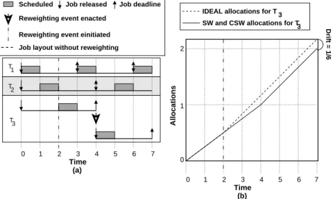
3.2 An example of the GEDF,IDEAL,CSW, andSW scheduling algorithms. . . . 68

(16)

3.4 A one-processor example of reweighting via Case (i) of Rule P underGEDF. . 73

3.5 A one-processor example of reweighting via Case (ii) of Rule P under GEDF. 73 3.6 A one-processor example of reweighting via Case (i) of Rule N underGEDF. . 75

3.7 A one-processor example of reweighting via Case (ii) of Rule N underGEDF. 75 3.8 A one-processor example of canceling a reweighting event. . . 77

3.9 A one-processor example ofNP-GEDF. . . 78

3.10 A one-processor example of task classes. . . 81

3.11 A one-processor example of task classes. . . 84

3.12 An example of the GEDF,IDEAL,CSW, and SWscheduling algorithms. . . . 87

3.13 A continuation of Figure 3.12. . . 88

3.14 An example of the EDF,IDEAL,CSW, and SWscheduling algorithms. . . 90

3.15 A partial schedule that illustrates drift when tasks miss deadlines. . . 95

3.16 A one-processor example of drift in NP-GEDF. . . 97

3.17 A one-processor example of drift in NP-GEDF. . . 98

4.1 An example of the MAOE,MROE, and AROEmetrics. . . 106

4.2 A one-processor example of deadlines when minimizing the MROE. . . 112

4.3 A one-processor example of thePEDF and SWscheduling algorithms. . . 114

4.4 A one-processor example of thePEDF and SWscheduling algorithms. . . 115

4.5 A one-processor example of reweighting via Case (i) of Rule P underPEDF. . 119

4.6 A one-processor example of reweighting via Case (ii) of Rule P under PEDF. . 119

4.7 A one-processor example of reweighting via Case (i) of Rule N underPEDF. . 121

4.8 A one-processor example of reweighting via Case (ii) of Rule N underPEDF. 121 4.9 A one-processor example of canceling a reweighting event. . . 122

4.10 A one-processor example of NP-PEDFreweighting. . . 123

4.11 A two-processor example of resetting under PEDF. . . 125

4.12 An illustration of t1 andtd. . . 132

4.13 An illustration of tz and ǫz. . . 133

4.14 An example illustrating the the NP-PEDFtardiness bound. . . 135

4.15 An example of the PEDF,IDEAL,CSW,SW,PTscheduling algorithms. . . . 137

(17)

4.16 A continuation of Figure 4.15. . . 138

4.17 An example of the PEDF,IDEAL,CSW,SW, and PTscheduling algorithms. . 139

4.18 A one-processor example of the task decomposition in Lemma 4.4. . . 146

4.19 A one-processor example of multiple reweighting events. . . 152

4.20 Decomposition of a task for Lemma 4.7. . . 155

4.21 Decomposition of a task for Lemma 4.9. . . 160

4.22 A one-processor example of drift in NP-PEDF. . . 169

4.23 A one-processor example of drift in NP-PEDF. . . 170

5.1 The behavior of a periodic andIStask. . . 178

5.2 The behavior of a periodic heavy task. . . 181

5.3 Pseudo-code definingA(_IIS,T_i[j],t). . . 182

5.4 Per-slot allocations forAISsystem. . . 185

5.5 An illustration of freeing the capacity. . . 187

5.6 A one-processorPD2 schedule of two tasks. . . 188

5.7 Pseudo-code defining theA(_SW,T_i[j],t). . . 189

5.8 An illustration of Rule P under PD2. . . 192

5.9 An illustration of Rule N underPD2. . . 193

5.10 An example of instant reweighting causing a heavy task to miss its deadline. 194 5.11 An example of increasing the weight of a heavy-changeable task. . . 196

5.12 An example of decreasing the weight of a heavy-changeable task. . . 197

5.13 An example of decreasing the weight of a heavy-changeable task. . . 198

5.14 An illustration of theAGIS task model. . . 205

5.15 The behavior of a periodic heavy task in an AGIS system. . . 206

5.16 The reweighting rules in an AGISsystem. . . 207

5.17 An example of a heavy-changeable task in an AGIS system. . . 208

5.18 An illustration of displacements. . . 209

5.19 Illustrating the sets A, B, and I. . . 215

5.20 An illustration of displacements caused by remove X(1). . . 216

(18)

5.22 An illustration of the proof of Lemma 5.13. . . 222

5.23 An illustration of Tx Lemma 5.14. . . 225

5.24 An example of the IDEALalgorithm underPD2. . . 232

5.25 An illustration of why PD-LJis coarse-grained. . . 233

5.26 An illustration that all EPDF algorithms incur drift. . . 234

5.27 An illustration of Rule P under PD2. . . 236

5.28 An illustration of Rule N under PD2. . . 237

5.29 An illustration of Rule N under PD2. . . 238

6.1 Estimated weight vs. importance value/service level. . . 249

6.2 The AGEDFscheduling algorithm. . . 251

6.3 A feedback system’s response to a step input. . . 252

6.4 Estimated weight vs. importance value/service level. . . 259

6.5 An illustration of changing the code segment. . . 262

7.1 The Whisper system. . . 265

7.2 Pseudo-code defining correlation. . . 266

7.3 An illustration of correlation. . . 267

7.4 An illustration of the Kalman Filter. . . 269

7.5 The core loop in Whisper. . . 270

7.6 An illustration of an occluding object. . . 270

7.7 Example of different methods for removing noise from a pixel. . . 273

7.8 The flow diagram of the VEC. . . 277

7.9 The VEC system divided into tasks. . . 279

7.10 The simulated Whisper system. . . 286

7.11 Whisper simulations. . . 287

7.12 Whisper simulations continued. . . 288

7.13 The simulated VEC system. . . 289

7.14 VEC simulations. . . 291

7.15 VEC simulations, continued. . . 292

(19)

7.16 The simulated Whisper system. . . 294

7.17 The actual weight of a Whisper task at three different service levels. . . 296

7.18 AGEDF running Whisper Continued. . . 297

7.19 AGEDF running Whisper. . . 298

7.25 The simulated VEC system. . . 304

7.26 The actual weight of a VEC task at three different service levels. . . 305

7.27 The actual weight of a VEC task at three different service levels. . . 306

7.28 AGEDF running VEC. . . 307

(20)

LIST OF ABBREVIATIONS

AIS Adaptable Intra-Sporadic Task Model

AGIS Adaptable Generalized Intra-Sporadic Task Model

AGEDF Adaptive GEDF

AAOE Average Absolute Overall Error

AROE Average Relative Overall Error

EDF Earliest-Deadline-First

EPDF Earliest-Pseudo-Deadline-First

EEVDF Earliest-Eligible-Virtual-Deadline-First

FF Fairness Factor

FCS Feedback-Control Real-Time Scheduling

FMLP Flexible Multiprocessor Locking Protocol

GEDF Global EDF

IS Intra-Sporadic

MAOE Maximal Absolute Overall Error

MROE Maximal Relative Overall Error

NP-GEDF Non-Preemptable GEDF

NP-PEDF Non-Preemptable PEDF

PEDF Partitioned EDF

RBED Rate-Based Earliest-Deadline

RTOS Real-Time Operating System

RAD Reasonable Allocation Decreasing

UA Average Under Allocation

(21)

CHAPTER 1

INTRODUCTION

The goal of this dissertation is to extend research on multiprocessor real-time systems in order

to enable such systems toadapt tasks’ processor shares—a process calledreweighting—in

re-sponse to both external and internal stimuli. The particular focus of this work is on adaptive

systems that are deployed in environments in which tasks may frequently require significant

share changes. Such environments are commonplace in computationally-intensive multimedia

applications. Prior to the research in this dissertation, no multiprocessor reweighting

algo-rithms had been proposed that could change task shares with bounded overhead. In this

dissertation, we extend prior work on uniprocessor and multiprocessor systems to construct

reweighting algorithms with minimal overhead for several different types of multiprocessor

systems. Furthermore, we examine how feedback and optimization techniques can be use to

determine, at run time, which reweighting events are needed. Finally, we evaluate the

pro-posed adaptive scheduling algorithms by using two multimedia applications developed at The

University of North Carolina at Chapel Hill: the Whisper human tracking system (Vallidis,

2002) and theVirtual Exposure Camera (VEC) night vision system (Bennett and McMillan,

2005).

To motivate the need for adaptive real-time scheduling, we begin this chapter with a brief

overview of Whisper and VEC. Next, we discuss the core real-time concepts that are relevant

to this dissertation. We then review prior work on adaptive real-time systems and state

(22)

1.1 Applications

Brief descriptions of Whisper and VEC are provided below; more detailed descriptions will be

given later in Chapter 7, where our experimental results are given. Before discussing Whisper

and VEC, it is important to point out that, since each is a multimedia application, both

must ensure certain timing constraints to provide an acceptable user experience and thus are

examples ofreal-time application. One of the questions we will answer in this dissertation is

how the timing constraints of real-time applications can be changed at run time while still

providing an acceptable quality-of-service (QoS).

1.1.1 Whisper

As mentioned above, Whisper performs full-body tracking in virtual environments (Vallidis,

2002). Whisper tracks users via an array of wall- and ceiling-mounted microphones that

detect signals (i.e., white noise) emitted from speakers attached to each user’s hands, feet,

and head. Specifically, by calculating the time-shift in the signal for each microphone-speaker

pair, Whisper is able to triangulate each speaker’s position. The amount of time required to

calculate the distance between a microphone-speaker pair is indirectly related to the

noise ratio. As the distance between a microphone-speaker pair increases, the

signal-to-noise ratio decreases, which increases the amount of time required to calculate this distance.

Also, other factors, like ambient noise, further degrade the signal-to-noise ratio causing total

computation time to increase. Because the computational cost associated with calculating

the distance between a microphone speaker-pair can change at run time, the tasks comprising

Whisper must be scheduled using algorithms that either allow task parameters to adapt or

allow task shares to be defined based on worst-case scenarios. Unfortunately, provisioning the

system based on worst-case scenarios may not be a viable option because there exist scenarios

for which no reasonable computational platform can correctly track a user (e.g., a room with

a 100dB of ambient noise). While using adaptive techniques reduces the resources required

to correctly track a user (relative to over-provisioning), the workload is still intensive enough

to necessitate a multiprocessor system.

(23)

1.1.2 Virtual Exposure Camera

The second application considered in this dissertation is the VEC video-enhancement

sys-tem (Bennett and McMillan, 2005).1 _{VEC is capable of improving the quality of an}

under-exposed video feed so that objects that are indistinguishable from the background become

clear and in full color. In VEC, darker objects require more computation to correct. Thus, as

dark objects move in the video, the processor shares of the tasks assigned to process different

areas of the video will change. Like all multimedia applications, to create an acceptable user

experience, VEC must update the corrected image at a regular rate. VEC will eventually

be deployed in a full-color night vision system, so tasks will need to change shares as fast

as a user’s head can turn. In the planned configuration, a multicore platform consisting of

approximately ten processing cores will be used.

1.2 Real-Time Systems

The distinguishing characteristic of a real-time system is the need to satisfy timing constraints.

The timing constraints of recurrent applications (e.g., Whisper and VEC) can be represented

using thesporadic task model. In this model, each piece of sequential recurrent code is called

atask. Each invocation of such a task is called ajob. We denote theith

task of a set of tasksT

asTi (where tasks are ordered by some arbitrary method), and denote thejth job of the task

Ti asT_ij (where jobs are ordered by the sequence in which they are invoked). Associated with

a sporadic task is aworst-case execution time (WCET), denotede(Ti), and aperiod, denoted

p(Ti). The WCET denotes the maximum amount of time any job of the task requires; the

period denotes the minimum separation between consecutive job invocations and defines a

relative “deadline” for each job. The time at which a job is invoked is called its release time,

denoted r(T_ij), and the (absolute) time by which a job must complete is called its deadline,

denotedd(T_ij). Theweight of a taskTi, denotedwt(Ti), is the fraction of a process it requires

to be correctly scheduled and is defined as e(Ti)/p(Ti). For shorthand, we will use Ti:(e, p)

to denote a taskTi with a WCET of eand a period ofp.

1_{In prior work (Block and Anderson, 2006; Block et al., 2008a; Block et al., 2008b), we referred to VEC}

(24)

11 5

4 3 2 1 T1

T2

T3

0 6 7 8 9 10

Scheduled

:(4,14) :(1,7/3) :(2,7)

Job release

Job deadline Job deadline & release

Time 12 13 14 15

Figure 1.1: A one-processor example with three sporadic tasks.

The release and deadline of the job T_ij of a sporadic task Ti can be specified as

r(T_i1) = θ(T_i1)

r(T_ij) = d(T_ij−1) +θ(T_ij), j >1

d(T_ij) = r(T_ij) +p(Ti), j≥1

where θ(T_ij) _≥ 0 for j _≥1. θ(T_ij) denotes the sporadic separation between job releases. If θ(T_ij+1) = 0, thenT_ij+1 is released atT_ij’s deadline.

Example (Figure 1.1). Consider the example in Figure 1.1, which depicts a one-processor system with three tasks: T1:(2,7), which has a sporadic separation of one time unit between

T₁1andT₁2;T2:(1,7/3); andT3:(4,14). The grey boxes denote the time at which the associated

job is scheduled. Down arrows denote a job release. Up arrows denote a job deadline.

Up-and-down arrows denote that a job’s deadline and its successor’s release occur at the same

time. Similar notation will be used in later figures.

The actual execution time of jobT_jj, denoted Ae(T_ij), is the amount of time for which T_ij

is scheduled; this value is upper-bounded bye(Ti). Depending on the scenario, this value may

or may not be known before the job finishes execution. To facilitate further discussion, a few

additional terms need to be defined.

Definition 1.1 (Window, Active, and Inactive). If T_ij is a job in the task system T, then thewindow ofT_ij defined as the range [r(T_ij),d(T_ij)). Furthermore, the job T_ij isactive

correct.

(25)

at time t iff t is in T_ij’s window (i.e., t _∈ [r(T_ij), d(T_ij))), and inactive otherwise. We use

ACT(t) to denote the set of active jobs at time t.

For example, in Figure 1.1,T₁1 is active over the range [1, 7) and is inactive at every other

time.

Definition 1.2 (Completed). If _S is a schedule of the task system T, then a job T_ij _∈T is said to have completed by time t in _S iff T_ij has executed for Ae(Ti) time units by t in S. Similarly, a task Ti is said to be complete at time t iff at time t every job of Ti that was

released byt has completed.

For example, in Figure 1.1, T₁1 is complete at and after time 4. Also, at time 10/3, T2 is

complete since both T₂1 and T₂2 are complete by time 10/3.

Definition 1.3 (Pending and Ready). For an arbitrary scheduling algorithm _A, if _S is a schedule of the task system T under _A, then a jobT_ij is said to bepending at time t in _S if

r(T_ij)_≤tand T_ij is incomplete att in_S. Note that a job can be both pending and inactive, if it misses its deadline. A pending job T_ij is said to be ready at time t in _S if all prior jobs of taskTi have completed byt. A job Tij can be pending but not ready if T

j−1

i is incomplete

at r(T_ij). (Such a scenario may occur in some multiprocessor algorithms.)

For example, in Figure 1.1, T₁1 is pending until time 4, and T₃1 is pending until time 11.

Let_Abe an arbitrary scheduling algorithm, τ be an arbitrary task system, and_S denote schedule of τ generated by _A. Then, we useA(_S,T_ij,t1,t2) denote the total time allocated to T_ij in _S in [t1,t2). Similarly, we use A(S,Ti,t1,t2) and A(S,τ,t1,t2), respectively, to denote the total time allocated to all jobs ofTi inS and all tasks ofτ inS, over the interval

[t1,t2). We say that the value of A(S,T_ij, 0,t) is the amount thatT_ij hasexecuted by t. For example in Figure 1.1,A(_S,T1

1, 0, 2) = 1 andA(S,T11, 1, 4) = 2.

Depending on the consequences of missing a deadline, real-time systems can be classified

as either “hard” or “soft.” A system is ahard real-time (HRT) system if missingany deadline

implies that the system fails. In contrast, in asoft real-time (SRT) system, deadlines may be

missed. Examples of HRT systems include avionics and automotive applications. Examples

(26)

miss an occasional deadline, it is still possible for such systems to “fail;” however, there is no

single notion of a “correct” SRT system. Some possible notions of SRT correctness include:

boundeddeadline tardiness (i.e., all jobs complete within some bound of their deadline) (Devi

and Anderson, 2008); a specified percentage of deadlines must be met (Lu et al., 2002); and

mout of everykconsecutive jobs of each task complete before their deadline (Hamadoui and

Ramanathan, 1995). In this dissertation, we are primarily concerned with HRT systems and

SRT systems with bounded deadline tardiness. For HRT systems, we say that a given task set

isschedulable if it is possible to guarantee that no single task will miss its deadline; otherwise

we say that it is unschedulable. Similarly, for SRT systems, we say that a given task set is

schedulable if it is possible to guarantee that every task has bounded deadline tardiness, and

is unschedulable otherwise. Moreover, for many types of system, we can determine if a given

task set is schedulable using a scheduability test, i.e., a set of conditions that, when satisfied

by the task set, imply that it is schedulable.

1.2.1 Uniprocessor Systems

The weight of a task can be used to define an ideal schedule, in which, at each instant,

each task is allocated a fraction of a processor equal to its weight. While the ideal schedule

represents the most equitable allocation of resources possible, it is infeasible to implement

since it requires tasks to be preempted and swapped at arbitrarily small intervals. For a

uniprocessor system, a more realistic scheduling algorithm is theearliest-deadline-first (EDF)

algorithm, which schedules jobs based on their deadlines, with earlier deadlines having higher

priority. On a uniprocessor system, EDF can guarantee that every job completes before its

deadline if the total weight of all tasks is at most one, the total available utilization.

Example (Figure 1.2). Figure 1.2 depicts a one-processor example of an ideal and EDF

schedule of a system with four tasks: T1:(1,2); T2:(2,8); T3:(1,8); and T4:(1,8) T1. The

numbers in each box denote the fraction of the processor consumed by the associated task.

Insets (a) through (c) depict, respectively, an ideal schedule, anEDFschedule, and the actual

and ideal allocations forT1.

(27)

T

Time

0 8

Job release

Job deadline Job deadline & release Fraction X of the Processor Scheduing the Task

T1

T2

1 2 3 4 5 6 7 1 2 3 4 5 6 7 8

2

T X

(b)

T Allocations 1

:(1,2) :(2,8) 1 T (c) Ideal :(1,8) :(1,8) :(1,2) :(2,8) :(1,8) Actual 4 3 1 2 0 Time

0 2 3 4 5 6 7 8

:(1,8) 4 3 1 T T Time 0 (a) 4 3 T 1/8 1 1 1 1 1

1 1 1

1/2 1/2 1/2 1/2

1/4

1/8

Figure 1.2: A one-processor example of an (a) ideal and (b) EDF schedule, and (c) T1’s allocation in both.

1.2.2 Multiprocessor Partitioned Scheduling

Most multiprocessor scheduling algorithms can be classified as either partitioned or global.

Under partitioned algorithms, each task is permanently assigned to a specific processor and

each processor independently schedules its assigned tasks using a uniprocessor scheduling

al-gorithm. Alternatively, under global algorithms, a task may migrate among processors. The

advantage of partitioned approaches over global approaches is that they have lower

migra-tion/preemption costs. This is because, under partitioned approaches, tasks maintain cache

affinity for longer durations of time due to fewer task migrations than in global approaches.

The disadvantage of partitioned approaches is that such systems have inferior scheduability

conditions when compared to global approaches (as we shall see).

This section discusses the specifics of two partitioned scheduling algorithms: preemptive

and nonpreemptive partitioned EDF (abbreviated asPEDF andNP-PEDF, respectively).

Un-derPEDF andNP-PEDFeach processor is scheduled independently using theEDFscheduling

algorithm. The difference between them is that, under PEDF, a job can be preempted, and

underNP-PEDF, a job cannot be preempted.

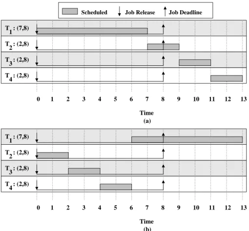
Example (Figure 1.3). Consider the example in Figure 1.3, which depicts a two-processor system with six tasks.: T1:(3,12);T2:(1,6);T3:(3,6); T4:(1,4); T5:(1,4); andT6:(5,12). Tasks

T1,T3, andT5 are assigned to Processor 1, and tasksT2,T4, andT6 are assigned to Processor

(28)

10 8 7

Job release

0 7 8 9 10

Time 6 (a) T 3 T 4 T 5 T 6 (b) Time 12 11 :(3,12) 1 T 6 12 11 Processor 1 :(5,12) :(1,4)

Processor 2 Job deadline

0 9 T T5 T4 T3 T2

1 2 3 4 5 :(1,4) :(3,6) :(1,6) :(3,12) 1 6 T :(5,12) T :(1,4) :(1,4) :(3,6) :(1,6) 5 4 3 2 1 2

Figure 1.3: Two-processor (a)PEDF and (b)NP-PEDF schedules.

Notice that, sinceT5 is assigned to Processor 1, Processor 2 is idle over the range [10, 11)

even thoughT5has work to be completed. Also note that the difference between Figure 1.3(a)

and Figure 1.3(b) is that in Figure 1.3(b) once a job begins executing it continues to do so

until it completes. This behavior is illustrated by T1

6, which has a contiguous execution in Figure 1.3(b) but not in Figure 1.3(a).

Before continuing, there is one subtlety that must be discussed. Throughout this

dis-sertation, whenever we discuss partitioned scheduling algorithms, we will make a distinction

between theguaranteed weightof a task and thedesired weightof a task (given bye(Ti)/p(Ti)).

This distinction is important because under partitioned algorithms, it is possible for a

pro-cessor to be over-allocated, i.e., the propro-cessor is assigned tasks with a total weight exceeding

one. When a processor is over-allocated, there are two options: reject one or more tasks; or

reduce the shares of the tasks on that processor. For example, in a two-processor system with

three tasks each of weight 2/3 (depicted in Figure 1.4), either one of the three tasks must be

rejected or the shares of the tasks on the over-allocated processor must be reduced. Both of

these options guarantee that the shares of tasks do not overutilize either of the processors

even though the weights do. While both variants have their relative advantages, for adaptive

systems, the latter option is likely a better option. (A thorough discussion of this is issue given

in Section 4.2.) It is important to note that for the majority of the algorithms considered in

(29)

3 T1 _T3 T2

Weight

Guaranteed

Weight

Guaranteed

1/3 2/3 3/3 4/3

Proc. 1 Proc. 2

T3 T2

Rejected

(c) (a)

1/3 2/3 3/3 4/3

Proc. 1 Proc. 2

Desired Weight

1/3 2/3 3/3

Proc. 1 Proc. 2

T

(b)

1

T1 T

T2

Figure 1.4: (a) A two-processor system with three tasks each with a desired weight of 2/3.

(b) The guaranteed weights of tasks in (a) when no task is rejected. (c) The guaranteed weights of tasks in (a) whenT2 is rejected.

this dissertation, a task’s guaranteed weight equals its desired weight. Thus, for brevity, we

will only use the terms “desired weight” and “guaranteed weight” when discussing algorithms

where the two may differ.

1.2.3 Restricted Global Multiprocessor Scheduling

In global scheduling algorithms, tasks are scheduled from a single priority queue and may

mi-grate among processors. Global algorithms can be further classified as either restricted and

unrestricted. A scheduling algorithm is considered to be restricted if the scheduling priority

of each job (for any given schedule) does not change once it has been released. A scheduling

algorithm is considered to be unrestricted if there exists a schedule in which some job changes

its priority after it is released. In this section, we discuss two restricted global scheduling

algorithms,preemptive global-EDF(GEDF) andnon-preemptive global-EDF(NP-GEDF);

unre-stricted algorithms are considered in Section 1.2.4. Under both GEDFand NP-GEDF, tasks

are scheduled from a single priority queue on anEDF basis. As with partitioned algorithms,

the only difference betweenGEDFandNP-GEDF is that jobs can be preempted inGEDFand

cannot be preempted in NP-GEDF.

Example (Figure 1.5). Consider the example in Figure 1.5, which pertains to a two-processor system with five tasks: T1:(2,7); T2:(1,7); T3:(1,7); T4:(3,7); and T5:(3,7). Inset

(a) depicts aGEDFschedule and inset (b) depicts anNP-GEDFschedule. In (a), T₅1 misses a

deadline by one time unit at time 7, and T₅2 misses a deadline by one time unit at time 14.

In (b),T₅2 misses a deadline by two time unit at time 14.

(30)

5 T 4 T 3 T 2 T 1 T (a)

Time 1112 13 1415

0 1 2 3 4 5 6 7 8 9 10

(b) 16 Time :(3,7) 15 :(2,7) 1 Processor 1 1 Job release Job deadline Processor 2 T :(3,7) :(3,7) :(3,7) :(3,7) 14 13 :(3,7) 12 11 :(3,7) 0 10 :(3,7) :(2,7) 5 T 9 8 7 4 T 3 6 T 2 5 T 4 3 2

Figure 1.5: Two-processor (a)GEDF and (b)NP-GEDF schedules.

it is not possible for a processor to be over-allocated in the long term, provided that total

utilization is at mostm, the number of processors. However, short-term over-allocations that

cause deadline misses are possible. Nonetheless, as shown by Devi and Anderson (Devi and

Anderson, 2008), such misses are only by bounded amounts. The amount of time by which

a job misses its deadline is called its tardiness. For example, in Figure 1.5(a), T₅1 misses a

deadline at time 7, and in both Figure 1.5(a) and Figure 1.5(b),T₅2 misses a deadline at time

14. As shown in (Devi and Anderson, 2008), underGEDF, the maximal tardiness of any job

of task aTi is bounded by a formula given shortly; however, before presenting their equation,

we briefly introduce a few needed terms. Letemindenote the minimum execution time of any

task in the systemτ. Define WT(τ) as

WT(τ) = X

Ti∈τ

wt(Ti).

Additionally, let maxe(k) and maxwt(k) denote, respectively, the kth largest execution time

and weight of any task. Finally, let the value Γ denote

Γ =     

WT(τ)₋1, WT(τ) is integral

⌊WT(τ)_⌋, otherwise.

Using these terms, the maximal tardiness (as given in (Devi and Anderson, 2008)) for any

(31)

job of a task Ti is given as

PΓ

k=1maxe(k)−emin

m₋PΓ−1

k=1maxwt(k)

+e(Ti), (1.1)

providedWT(τ)_≤m, wheremis the number of processors. Since tasks cannot be preempted inNP-GEDF, its tardiness bound is slightly larger than (1.1). (See (Devi and Anderson, 2008)

for details.)

1.2.4 Unrestricted Global Multiprocessor Scheduling

The final multiprocessor scheduling algorithm we consider in this dissertation is the

unre-stricted global Pfair algorithm PD2 (Srinivasan and Anderson, 2005). PD2 schedules a task

by breaking it into a sequence in which of subtasks, each of which represents one time unit

of execution. Each such time unit is called a quantum. The jth

subtask of the task Ti is

denoted asT_i[j], where subtasks are ordered by the sequence in which they are invoked.

Asso-ciated with each subtask is apseudo-release and pseudo-deadline (often called “release” and

“deadline” for brevity), which are defined as

r(T_i[1]) = θ(T_i[1])

r(T_i[j]) = d(T_i[j−1]) +

j₋1

wt(Ti)

−

j₋1

wt(Ti)

+θ(T_ij), j >1

d(T_i[j]) = r(T_i[j])₋

j₋1

wt(Ti)

+

j

wt(Ti)

, j_≥1

where θ(T_i[j]) _≥ 0 for j _≥ 1. θ(T_i[j]) denotes the “sporadic” separation between subtask releases (such separations are called “intra-sporadic”). PD2 schedules subtasks on an

earliest-pseudo-deadline-first basis with two tie-breaking rules, which are used in the event of a

dead-line tie. (A more thorough discussion ofPD2 can be found in Chapter 5.) Since tasks inPD2

are scheduled one quantum at a time, a task’s execution time is assumed to be a multiple of

the quantum size (and must be rounded up if this is not the case) and the scheduling of a

task depends only on its weight. The main advantage of PD2 over all other aforementioned

algorithms is that PD2 is the only algorithm that can guarantee that every job is scheduled

before its deadline and no processor is over-allocated provided total utilization is at most

(32)

T T 2 T 1 T

Time

0 1 2 3 4 5 6 7 8 111213 14

Subtask release Subtask deadline

Processor 2 Processor 1

:(3,7) :(3,7) :(3,7) :(3,7) :(2,7)

5 T 4 3

9 10

Figure 1.6: A two-processor system scheduled by PD2.

possible that a task will be preempted and migrated every quantum, which can cause tasks to

incur large migration/preemption costs. Another disadvantage ofPD2 is that task execution

times must be rounded up, which can cause the system to be underutilized. For example, if

a task has an execution time of 3.1 and a period of 4, then its weight would be 4/4 = 1, since

the execution time of 3.1 would be rounded up to one.

Example (Figure 1.6). Figure 1.6 shows aPD2 schedule for the task system consider earlier in Figure 1.5.

Notice that, in this schedule, tasks are scheduled one quantum at a time. As a result,

tasks may be preempted at the end of every quantum and may migrate nearly as frequently.

Also note that a subtask (unlike a job) may be released before the deadline of its successor.

Finally, notice that, in this schedule, every task is scheduled before its deadline and that tasks

with the same weight (but different periods) receives allocations at the same rate, e.g., T3

and T4 receive approximately one allocation in any 7/3-quantum interval.

1.2.5 Impact of Migrations and Preemptions

Given these five algorithms, it is obvious that in the absence of migration and preemption

costs, PD2 should be the preferred algorithm since it is the only algorithm that can both

guarantee that every job completes before its deadline and that the share of every task equals

its weight. However, for many applications, migration and preemption costs may be

(33)

stantial. Recently, our research group (Calandrino et al., 2006) constructed a multiprocessor

testbed, called LITMUSRT, to compare different real-time scheduling algorithms. We then

used this testbed to implement all of the aforementioned algorithms (except NP-PEDF) on a

four-processor system (with 2.7 GHz processors) in an effort to assess the impact of migration

and preemption costs. In our work, we varied the weight of tasks being scheduled and the

amount of cache used by each task. (Migrations and preemptions cause a loss of cache affinity,

and as a result, if a task utilizes a larger fraction of the cache, then that task has both higher

migration and preemption costs.)

Our experiments assessed the performance of each algorithm as measured by the number

of processors that would be required to schedule a number of randomly generated task sets

with a maximal utilization of four. These experiments showed the following:

• The HRT performance ofPEDFandGEDFimprove (relative to the other algorithms) as migration and preemption costs increase and/or the weights of tasks decrease. However,

PEDF always has better HRT performance thanGEDF.

• The performance ofPD2 improves (relative to the other algorithms) as migration and preemption costs decrease and/or the weights of the tasks increase.

• PD2 has virtually the same performance in both HRT and SRT systems.

• PEDFhas virtually the same performance in both HRT and SRT systems.

• BothGEDFandNP-GEDFalways perform better than any other algorithm for SRT

sys-tems. Furthermore,NP-GEDF has slightly better performance than GEDF. (The HRT

performance ofNP-GEDF was not considered since there does not exist a scheduability

test for it that would return meaningful results.)

The reason why the performance ofPEDF is adversely impacted by increasing task weights is

that, if tasks have higher weights, then it is harder to produce a valid partitioning. Similarly,

for GEDF, as task weights increase, it becomes more likely that a job will be tardy. As a

result, additional processing capacity is needed to prevent such a scenario. The performance

(34)

tasks with larger weights in consecutive quanta, thus reducing the number of migrations and

preemptions. GEDF andNP-GEDF perform well for SRT systems because even though these

algorithms can cause tasks to miss deadlines, they incur relatively little migration/preemption

cost. Moreover, since tasks are not partitioned underGEDFand NP-GEDF, the performance

(in terms of the required number of processors to guarantee bounded tardiness) does not

substantially degrade as task weights increase. Given these results, it is easy to see that

there there does not exist a single “best” multiprocessor scheduling algorithm, and the choice

of which algorithm depends on the scenario in which it will be used. The theoretical and

empirical results from this section are summarized in Tables. 1.1 and 1.2, respectively.

1.2.6 Research Needed

Under traditional task models (e.g., the sporadic model), the scheduability of a system is

based on each task’s WCET. The disadvantage of using WCETs is that a system may be

deemed unschedulable even if it would function correctly most (or possibly all) of the time

when deployed. Adaptive real-time scheduling algorithms allow per-task processor shares

to be adjusted based upon run time conditions, instead of always using constant share

al-locations based upon WCETs. Prior to the research in the dissertation, for multiprocessor

systems, one approach for reweighting a task had been proposed, as we will discuss in

Sec-tion 2.1 (Srinivasan and Anderson, 2005); however, this approach only allows tasks to reweight

at job boundaries. By delaying a task’s reweighting request until its next job boundary, the

system may “drift” from its “ideal” allocation by an arbitrarily large amount. As a result, for

applications like Whisper and VEC, where timing constraints are continually changing, such

delays may cause unacceptably poor performance. In this dissertation, we remedy this

short-coming by proposing a set of rules that allow tasks to reweight without causing unbounded

drift, and an adaptive framework that determines at run time which adaptions are needed.

(35)

Scheme Desired = Guaranteed Weight Guaranteed Deadlines

PEDF No Yes

NP-PEDF No No

GEDF Yes No

NP-GEDF Yes No

PD2 Yes Yes

Scheme Migrations Preemptions

PEDF Never At Job Completions and Releases

NP-PEDF Never Never

GEDF At Job Completions and Releases At Job Completions and Releases

NP-GEDF In Between Jobs Never

PD2 Every Quantum Every Quantum

Table 1.1: Summary of algorithms and their properties. Note that deadlines can be guaranteed underPEDFonly at the expense of allowing guaranteed weights to be less than desired weights.

Scheme Light Tasks Heavy Tasks

(Hard) (Hard) (Hard)

PEDF Best Poor

GEDF Good Worst

NP-GEDF N/A N/A

PD2 Worst Best

Scheme High Mig./Preemp. Costs Low Mig./Preemp. Costs

(Hard) (Hard) (Hard)

PEDF Best Poor

GEDF Good Worst

NP-GEDF N/A N/A

PD2 Worst Excellent

Scheme Soft-Real Time

(All cases)

PEDF Same as hard

GEDF Excellent

NP-GEDF Best

PD2 Same as hard

(36)

1.3 Adaptivity

This section provides a review of prior work on adaptive uniprocessor real-time schemes in

which tasks are reweighted based on external and internal stimuli.

1.3.1 Leave/join Reweighting

Underleave/join reweighting (Srinivasan and Anderson, 2005), a task’s weight is changed at

job boundaries by forcing it to leave with its old weight and rejoin with its new weight.

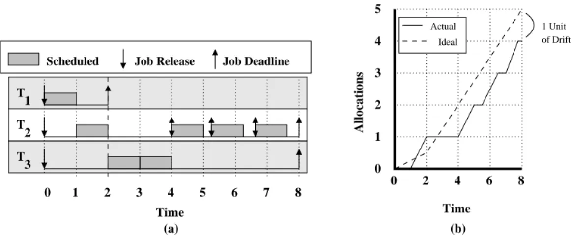
Example (Figure 1.7). Consider the example Figure 1.7, which depicts a one-processor system with three tasks: T1:(1,2) that leaves at time 2;T2, which has an initial weight of 1/4,

an execution cost of 1, and “initiates” a weight increase at time 2 to a weight of 3/4, which is

enacted by leave/join reweighting atT₂1’s deadline (i.e., time 4); andT3:(2,8). (a)illustrates theEDFschedule and(b) illustrates the ideal and actual allocations to taskT2.

Notice that, even though T2 “initiates” its change at time 2 and capacity exists for T2 to

increase its weight, this weight change cannot be “enacted” until its deadline. This illustrates

that the primary drawback to leave/join reweighting is that a task canonlychange its weight

at job boundaries. As a result, over the time range [2, 4),T2 behaves as though it is a task

of weight 1/4, even though in the ideal system (which can instantly enact weight changes) T2

would behave as a task of weight 3/4, is depicted in Figure 1.7(b). As a result,T2’s allocation

in the actual schedule “drifts” from its allocation in the ideal schedule by one time unit.

(Briefly,drift is the difference between a task’s ideal and actual allocations caused by a single

reweighting event.) Moreover, since leave/join reweighting cannot enact a reweighting event

until a job boundary, it is possible that a task can incur an arbitrarily large amount of drift

for one reweighting event. Section 1.5.3 provides a more detailed discussion concerning drift.

1.3.2 Rate-Based Earliest Deadline

Under rate-based earliest-deadline (RBED) scheduling (Brandt et al., 2003), which was

pro-posed for uniprocessor systems, tasks are scheduled on an EDF basis and can change their

(37)

1

3 T

2 T

T

Job Deadline

(b) Time (a)

Allocations

5

4

3

1

0 3

Scheduled Job Release

2

8 6 4 2 0

Time

8 7 6 5

0 1 2 4

1 Unit of Drift Ideal

Actual

Figure 1.7: The (a) EDF schedule and the (b) ideal and actual allocations to T2 in a one-processor example of leave/join reweighting.

weights and periods via two different rules based on whether the execution time or period is

changed. While these rules are more responsive than leave/join reweighting, it is still possible

for a task to incur an arbitrarily large amount of drift underRBED. In Chapter 2, we will

review this work in detail.

1.3.3 Proportional Share Scheduling

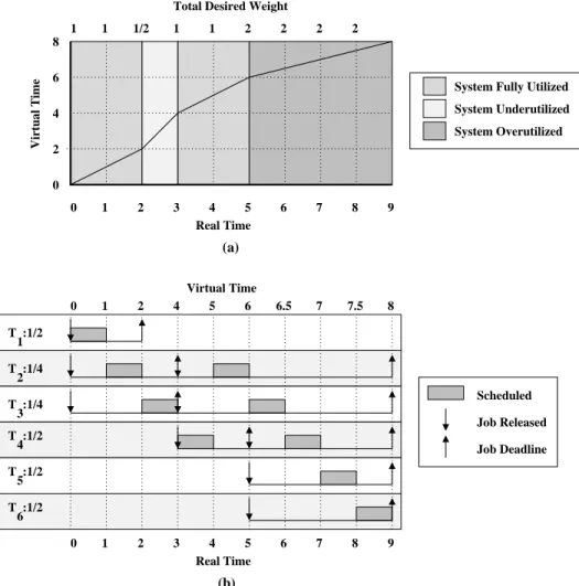
Underproportional share scheduling (Stoica et al., 1996), the guaranteed weight of each task

is determined as a function of its desired weight and the desired weight of all other tasks.

Specifically, the guaranteed weight of the taskTi at time tis defined as

Gwt(Ti, t) =

wt(Ti)

WT(τ,t), (1.2)

where WT(τ,t) is the total desired weight of all active tasks in the system τ at time t. For

example, consider a one-processor system that consists of four tasks: T1 that has a desired

weight of 1/2; T2 that has a desired weight of 1/4;T3 that has a desired weight of 1/4; and

T4 that has a desired weight of 1/8. If, at some time t1 all four tasks are active, then the

guaranteed weight for each task would be 1/(1/2 + 1/4 + 1/4 + 1/8) = 8/9 of its desired

weight. So, the desired weight of T1 would be 4/9. Alternatively, if at some time, t2, only

T1 andT2 were active, then the guaranteed weight of each would be 4/3 of its desired weight

for each task. So, the guaranteed weight of T1 would be 2/3. It is worthwhile to note

(38)

without using leave/join techniques. In Section 2.3, we will review one of the more popular

proportional share scheduling algorithms.

1.3.4 Adaptive Feedback-Based Frameworks

In adaptive feedback-based scheduling algorithms, the execution time of each job is unknown

until it is complete. As a result, in these systems, each task’s weight is defined as a function

of its estimated execution time, which is calculated for a job by using the actual execution

times of the task’s prior jobs. Moreover, a user can fine-tune a feedback-based system to

achieve desired behaviors.

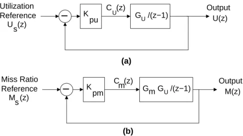
Lu et al. (Lu et al., 2000) were the first to propose such a scheduling algorithm, which

was directed at uniprocessor systems.2 Under their algorithm, called FC-EDF2, each task

has multiple versions (called service levels), each of which has a different level of QoS and

a different nominal processor share, representing the fraction of a processor the task will

require on average if it executes at that service level. A task can only execute at one service

level at a time. In order to control the system, FC-EDF2 monitors the system’s utilization

and miss-ratio, i.e., the fraction of jobs with missed deadlines. In order to minimize the

miss-ratio while maximizing utilization,FC-EDF2 adjusts the set of scheduled tasks and their

service levels. More recently, Lu et al. extended this work to create a comprehensive feedback

scheduling framework (Lu et al., 2002) that more explicitly incorporates the value to the

system associated with each service level. This framework is the basis for the approach we

propose in this paper. One drawback ofFC-EDF2 is that, because only the utilization and the

system-wide miss-ratio are monitored, the system cannot identify whether an individual task

has an actual execution time that deviates substantially from its estimated execution time.

Thus, the system can only respond to differences between the actual and estimated execution

times of tasks by changing the entire system instead of only a few tasks.

Alternatively, Abeni et al. have proposed a uniprocessor feedback algorithm in which each

task has its own feedback-controller rather than one controller for the entire system (Abeni

2_{Specifically, the first}_correct _{feedback algorithm was proposed in (Lu et al., 2000). The original system,}

FC-EDF_{, proposed in (Lu et al., 1999) could not satisfy its design specification because it was possible for the}

controller to become saturated, thus rendering it unable to correctly adjust the system.

(39)

et al., 2002). In order to attempt to maintain an accurate processor share for each task, their

algorithm monitors,for each task, the difference between the estimated and actual execution

times of each job. Once the system has calculated a new estimated execution time for a future

job, it adjusts the task’s weight. More recently, Cucinotta et al. extended this approach to

provide stochastic guarantees concerning per-task processor shares (Cucinotta et al., 2004).

One drawback of their approach is that it ignores the possibility that some tasks are more

important than others.

In addition to general-purpose real-time scheduling algorithms, feedback-based scheduling

has become increasingly important for managingcontrol tasks, i.e., tasks that control external

devices. In work by Mart´ı et al. (Marti et al., 2004), an approach is proposed that is similar

to that of Abeni et al., except that in (Marti et al., 2004), each period of each task has an

associated “importance value” that denotes the task’s value to the system in that period.

By using importance values, Mart´ı et al. determined the optimal period for each task via

standard linear programming techniques. One limitation of this approach is that it cannot

adjust the amount of time for which a task executes, like other approaches (e.g., like that of

Lu et al. (Lu et al., 2002)).

1.4 Thesis Statement

There are two major limitations of prior work on adaptive uniprocessor systems. First,

there does not exist a set of metrics for comparing different reweighting algorithms. Second,

existing methods for changing the weights of tasks (i.e., leave/join reweighting and RBED)

may give rise to an unacceptably long delay after initiating a weight change before it is

enacted. For multiprocessor systems, the limitations are even more severe since the only

method for changing the weight of a task is to use leave/join reweighting. Moreover, for

multiprocessor systems, there is an inherent tradeoff, which must be explored, between the

level of migration/preemption and the “accuracy” of the adaptive protocol. Also, there is

no global feedback-based adaptive framework, which would be necessary for implementing

applications like Whisper and VEC. The main thesis of this dissertation, which attempts to

(40)

Multiprocessor retime scheduling algorithms can be made more adaptive by

al-lowing tasks to reweight between job releases. Feedback and optimization techniques

can be used to determine at run time which reweighting events are needed. The

accuracy of such an algorithm can be improved by allowing more frequent task

mi-grations and preemptions; however, this accuracy comes at the expense of higher

migration and preemption costs, which impacts average-case performance. Thus,

there is a tradeoff between accuracy and average-case performance that will be

dependent on the frequency of task migrations/preemptions and their cost.

1.5 Contributions

In this section, we briefly discuss the contributions of this dissertation.

1.5.1 Adaptable Task Model and Reweighting Algorithms

The first contribution we discuss in the dissertation is the adaptable task model (originally

proposed in (Block et al., 2008b)). This model is an extension of the sporadic task model,

where the weight of each task T, wt(T,t), is a function of time t, and a task’s execution

time can vary between job releases. A task T changes weight or reweights at time t+ 1 if

wt(T,t)₆=wt(T,t+ 1). If a task T changes weight at a time tc between the release and the

deadline of some job T_ij, then the following two actions may occur:

(i) IfT_ij has not been scheduled by tc, thenTij may be “halted” at tc. (ii) r(T_ij+1) may be redefined to be less than d(T_ij).

In the sporadic model defined earlier, every job’s deadline is at or before its successor’s release.

As we will discuss in Section 1.5.2, the reason why the above two actions may occur is that

the value ofr(T_ij+1) may change as a result of a reweighting event. The reweighting rules we

present later in this section state the conditions under which the above actions may occur

and the number of time units befored(T_ij) that job T_ij+1 can be released.

As has already been discussed, when a task reweights, there can be a difference between

when it initiates the change and when the change is enacted. The time at which the change

(41)

is initiated is a user-defined time; the time at which the change is enacted is dictated by a

set of conditions that differ slightly for each type of multiprocessor reweighting algorithm.

Furthermore, the release and deadline of a job of an adaptable task is defined based on the

weight of the task when it was released.

1.5.2 Reweighting Rules.

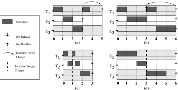
The second major contribution of this dissertation is the construction of reweighting rules

for PEDF, NP-PEDF, GEDF, NP-GEDF, and PD2. (The reweighting rules for PEDF, and

by extension forNP-PEDF, were proposed by Block and Anderson in (Block and Anderson,

2006); the reweighting rules forGEDFand NP-GEDFwere proposed by Block et al. in (Block

et al., 2008b); and the reweighting rules forPD2were proposed by Block et al. in (Block et al.,

2008a).) In all five reweighting algorithms, tasks change weight via one of two rules that are

based on whether a task’s active job is over- or under-allocated relative to an ideal schedule.

• If a task isunder-allocated, then the change is enacted by immediately halting the active job and releasing a new job with the remaining execution time.

• If a task is over-allocated, then one of two actions occurs: (i) if the task increases its weight, then the change is enacted by immediately halting the active job and releasing

the next job when the task’s “ideal” allocation equals its “actual” allocation; (ii)if the task decreases its weight, then the active job immediately halts and when the task’s

“ideal” allocation equals its “actual” allocation, the change is enacted and the next job

is released.

When aT_ij ishalted at timet,T_ij is not scheduled after time t.

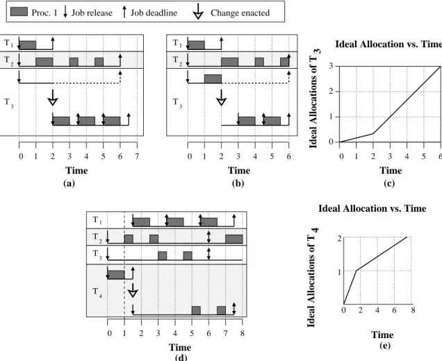
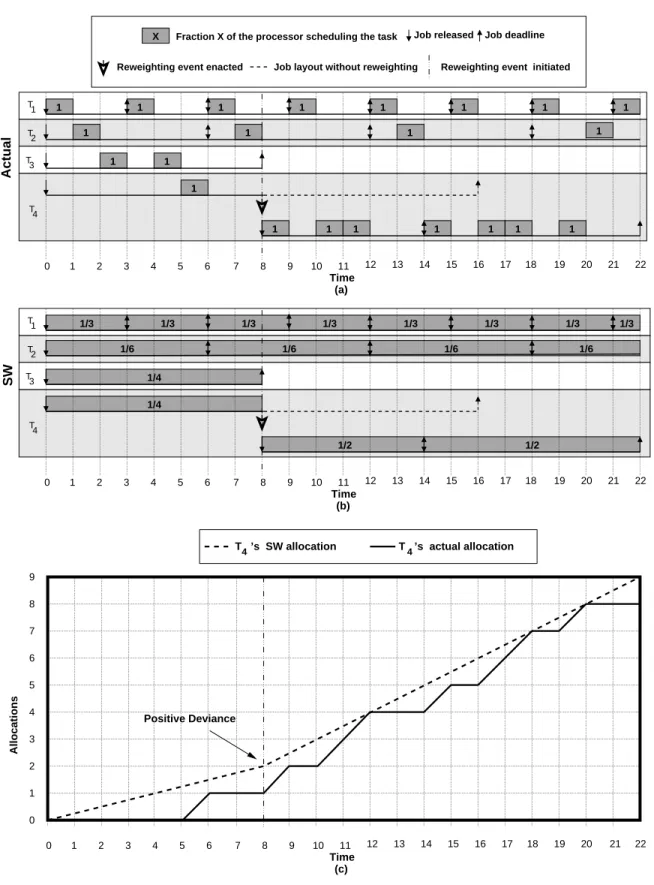
Example (Figure 1.8). Consider the examples depicted in Figure 1.8. Insets (a) and (b) pertain to a one-processor system with: T1:(1,2), which leaves the system at time 2;T2:(1,6);

andT3, with an execution cost of 3 and an initial weight of 1/6 that increases to 4/6 at time 2.

Since the first jobs of T2 andT3 have the same deadline, we can arbitrarily choose which job

has a higher scheduling priority. Inset (a) depicts the case where T2 has higher priority, and

(42)

Thus, when T3 reweights, its current job “halts” and its next job is immediately released.

Inset (b) depicts the case whereT3 has higher priority, and as a result,T3 is “over-allocated”

relative to the ideal system, when it reweights at time 2. Thus, whenT3 reweights, its current

job “halts” and its next job is not released until the difference between T3’s ideal and actual

allocations is zero (at time 3). The dotted lines denote the interval of the first job ofT3 that

has been changed by the reweighting event. Inset (c) depicts the ideal allocation of T3 as a

function of time. Notice that, at time 2, when T3 increases its weight from 1/6 to 4/6, the

ideal allocation rate increases from 1/6 to 4/6, and that at time 3, T3’s total ideal allocation

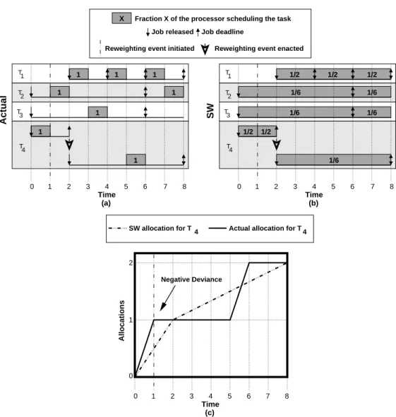
equals 1. Inset (d) depicts a one-processor system with four tasks: T1:(1,2), which joins

the system at time 1.5; T2:(1,6); T3:(1,6); and T4, which has an initial weight of 4/6 that

decreases to 1/6 at time 1. Since T4 is over-allocated at time 1 and decreases its weight, its

weight change is enacted when its ideal allocation equals its actual allocation (at time 1.5).

Inset (e) depicts ideal allocation forT4.

One important property of the above reweighting rules is that reweighting events are

task-independent. That is, if a task Ti changes its weight, thenonly the releases and deadlines of

jobs ofTi change. As a result of this independence, a task can only increase its weight at time

t if enough capacity for the reweighting event is available. For example, if a two-processor

task system has three tasks each of weight 0.6, then none of these tasks can initiate a weight

increase to 0.9 (since this would cause the system load to be 2.1), unless one of the other

two tasks first decreases its weight or leaves the system. (If reweighting events were not

task-independent, then it would be possible for a proportional-share scheduling algorithm to

increase the weight of a task at the expense of the shares of other tasks in the system.)

1.5.3 Evaluating Algorithms

The next contribution of this dissertation is a comparison of the reweighting algorithm for

dif-ferent multiprocessor scheduling frameworks. In order to evaluate the reweighting algorithms,

we use three different metrics: overload,tardiness, anddrift. Overload is the maximal amount

that a single processor is overutilized (assuming that the system is not overutilized). Tardiness

is the maximal amount by which a task can miss a deadline. Drift is the maximal amount of

(43)

Change enacted Job deadline

Job release Proc. 1

2 T

T

T T T

(a) (b) (c)

T T

T

Time (d)

Time (e)

0 1 2 3 4 5 6 7 0 1 2 3 4 5 6 0 1 2 3 4 5 6

1

0 2 3

T

Time Time Time

Ideal Allocation vs. Time

Ideal Allocations of T

0 1 2 3 4 5 6 7 8

T

Ideal Allocations of T

Ideal Allocation vs. Time

3

4

1

0 2 4 6 8

1 2

4 1 2

1 2

3

3 3

Figure 1.8: Several one-processor systems scheduled by EDF using our reweighting rules.

Adaptive multiprocessor real-time systems

ABSTRACT

ACKNOWLEDGMENTS

TABLE OF CONTENTS

LIST OF TABLES

LIST OF FIGURES

LIST OF ABBREVIATIONS

INTRODUCTION

1.1

Applications

1.2

Real-Time Systems

1.3

Adaptivity

1.4

Thesis Statement

1.5

Contributions