Raval_unc_0153D_16315.pdf

O

C

E

T

S

ON THE

C

E

Vivek Raval

A dissertation submitted to the faculty of the University of North Carolina at Chapel Hill in par-tial fulfillment of the requirements for the degree of Doctor of Philosophy in the Department of

Accounting.

Chapel Hill 2016

Approved by:

Wayne Landsman

Robert Bushman

Mary Barth

Eva Labro

Mark Lang

c 2016 Vivek Raval

ABSTRACT

VIVEK RAVAL: Organizational Capital and the Effects of Technology Shocks on the Characteristics of Earnings.

(Under the direction of Wayne Landsman and Robert Bushman)

The objective of this study is to hypothesize and test the effects that the introduction of new

productive technologies into an economy have on the characteristics of earnings. To do this, I

leverage theory from Eisfeldt and Papanikolaou (2013) that describes how economy-wide

tech-nology shocks affect the value of organizational capital, an important intangible asset. Because

organizational capital is largely unrecognized in financial statements, I hypothesize that periods of

technology shock are associated with lower earnings timeliness, particularly for firms with more

organizational capital. I also hypothesize that technology shocks are associated with more

sub-sequent goodwill impairment and restructuring, and that these associations are mediated by the

quantity or efficiency of the firm’s organizational capital. My findings support my hypotheses and

demonstrate how investment in organizational capital creates exposure to aggregate technology

ACKNOWLEDGMENTS

I thank my dissertation committee, Robert Bushman (co-chair), Wayne Landsman (co-chair),

Mary Barth, Eva Labro, Mark Lang, and Sean Wang. I also appreciate comments from Travis

Dyer, Atif Ellahie, John Hand, Bradley Hendricks, Preetesh Kantak, Nicholas Martin, Ed Maydew,

Jim Omartian, Lorien Stice-Lawrence, Ed Sul, Donny Zhao, workshop participants at Dartmouth

College, London Business School, the University of Arizona, the University of Colorado, the

Uni-versity of Illinois in Chicago, the UniUni-versity of North Carolina, Rice UniUni-versity, and participants

TABLE OF CONTENTS

LIST OF TABLES . . . vi

LIST OF FIGURES . . . vii

1 Introduction . . . 1

2 Conceptual Framework . . . 5

2.1 Organizational Capital and Technology Shocks . . . 5

2.2 Theory . . . 6

2.3 Operationalization of Technology Shocks and Organizational Capital . . . 10

2.4 Empirical Validation . . . 12

3 Hypothesis Development . . . 16

4 Research Design . . . 20

4.1 Tests of H1: Earnings Timeliness . . . 20

4.2 Test of H2: Goodwill Impairment . . . 24

4.3 Test of H3: Restructuring . . . 25

5 Data . . . 28

6 Results . . . 32

7 Conclusion . . . 36

A Tables . . . 37

B Figure . . . 48

LIST OF TABLES

A.1 Aggregate Means by Year . . . 37

A.2 Descriptive Statistics of Annual Aggregate Variables . . . 39

A.3 Correlations of Annual Aggregate Variables . . . 40

A.4 Descriptive Statistics - Panel Samples . . . 41

A.5 Aggregate Earnings Timeliness and Technology Shocks . . . 43

A.6 Earnings Timeliness and Technology Shocks by Level of Organi-zational Capital . . . 44

A.7 Relation Between Current Returns and Future Earnings Condi-tional on Technology Shock . . . 45

A.8 Goodwill Impairment and Technology Shocks . . . 46

LIST OF FIGURES

B.1 A graphical representation of the value of components of

CHAPTER 1: INTRODUCTION

In the right circumstances, the match between an employee and firm can generate value for

the firm. However, employees are also free to leave their firms and ultimately control how they

spend their time. These points underlie two important implications. First, because employees

are not controllable by the firm, they are not accounted for as assets of the firm, creating a gap

between firm value and the book value. Second, because employees may leave at will, the value

that certain employees bring to a firm is at risk. This study investigates how these two implications

interact during times of macro-economic shock to affect the dynamics of earnings timeliness and

write-downs in earnings over time.

Organizational capital is an economically significant intangible asset that is created from the

combination of a firm’s technologies and key talent. Technologies are processes and systems that

determine the efficiency with which a specific firm conducts its business. Key talent are the

highly-skilled labor inputs that have the general education, experiences, and skills to deploy and manage

technologies. Because organizational capital is based on both the firm’s technologies and key

talent, both the firm’s shareholders and key talent have a claim to its value. In order to sustain

organizational capital in a firm, the shareholders and key talent must share the value generated by

organizational capital.

Aggregate, or economy-wide, technology shocks introduce more efficient processes and

sys-tems, and create large-scale potential for more efficient firms. This makes key talent more valuable

in the economy, increasing their bargaining power, and changing how the value of organizational

capital is shared between key talent and shareholders. Because shareholder’s value in

organi-zational capital fluctuates based on undiversifiable economy-wide technology shocks, firms with

organizational capital are exposed to systematic risk. This theory, attributable to Eisfeldt and

the aggregate economy can affect the value of an important intangible asset.

The objective of this study is to hypothesize and test how technology shocks can affect the

characteristics of earnings. I use Eisfeldt and Papanikolaou (2013) as a theoretical foundation on

which I construct my hypotheses. The theory has two main implications relevant to this study.

First, aggregate technology shocks reduce shareholders’ value in organizational capital. Second,

aggregate technology shocks increase the likelihood that firms reorganize around a new technology,

particularly if they are less efficient.

Based on the theorized outcomes in Eisfeldt and Papanikolaou (2013), I form three sets of

hy-potheses. First, I hypothesize that earnings is less timely in reflecting of contemporaneous changes

in value during times of aggregate technology shocks. Because internally-generated intangible

as-sets are generally off-balance sheet, organizational capital is also likely to be off-balance sheet (Lev

and Radhakrishnan 2005). When technology shocks reduce shareholders’ value in organizational

capital, the accounting system has no asset to write-down, so the accounting system will need to

re-flect the value through transactions over time, reducing its timeliness. Because technology shocks

affect earnings by changing the value of organizational capital, I expect the effect of technology

shocks on earnings to be stronger for firms with more organizational capital investment.

Second, because technology shocks reduce the value of organizational capital, I expect that

firms will record more goodwill impairment subsequent to technology shocks. Acquisition

ac-counting is a special case in which acquired internally-generated intangible assets may be

recog-nized on the balance sheet as acquired goodwill. Therefore, after acquisition, the purchase price of

organizational capital is part of the balance of acquired goodwill. Technology shocks reduce the

value of acquired organizational capital, triggering goodwill impairment. Because firms with more

organizational capital in goodwill are likely to record more impairment, I expect the effect of

tech-nology shocks on goodwill impairment to be stronger for firms with high levels of organizational

capital investment.

Third, because technology shocks increase the likelihood of reorganizing the firm around a

Adopting a new technology requires that a firm reorganize its processes and systems, and allows a

firm to increase its efficiency. This can result in the consolidation of facilities and the reduction or

relocation of labor. These costs are recognized as restructuring charges. Because firms that have

higher efficiency are less likely to restructure, I expect that the effect is lower for more efficient

firms.

My empirical strategy for identifying technology shocks is also grounded in the theory in

Eisfeldt and Papanikolaou (2013). A theorized outcome of technology shocks is that they

re-duce shareholders’ value in organizational capital. Accordingly, to identify periods of technology

shocks, I borrow from Eisfeldt and Papanikolaou (2013), and use a hedge portfolio that is designed

to measure the economy-wide industry-balanced returns to organizational capital. Low portfolio

returns indicate low organizational capital returns and periods of aggregate technology shock.

My results provide evidence consistent with my hypotheses. Using both an aggregate and

more firm-specific measure of earnings timeliness, I find that technology shocks are associated

with lower earnings timeliness, and that this is particularly the case for firms with higher

organi-zational capital. I also find evidence that goodwill impairments and restructuring charges increase

subsequent to technology shocks, and that this effect is stronger (weaker) firms with higher levels

of organizational capital investment (efficiency).

Findings from my study shed light on how the dynamics of the aggregate economy affect the

time-series and cross-sectional variation in the characteristics earnings. This study speaks to the

call for research on the interaction between the fundamental drivers of firm performance and

earn-ings quality (Dechow, Ge, and Schrand 2010). Also, because this study focuses on organizational

capital, findings can contribute to the literature on intangible assets. Specifically, studies such

as Srivastava (2014); Lev and Zarowin (1999) imply that investment in intangible assets expose

firms to fluctuations in value that are not well measured by earnings. My study demonstrates one

way in which investment in a specific intangible asset, organizational capital, can expose firms to

The remainder of this paper is organized as follows. Chapter 2 outlines the theory

describ-ing how technology shocks affect shareholders’ value in organizational capital, and describes how

these constructs are operationalized. Chapter 3 develops hypotheses, Chapter 4 develops the

re-search design, Chapter 5 describes the data, and Chapter 6 presents the results. Chapter 7 concludes

CHAPTER 2: CONCEPTUAL FRAMEWORK

2.1 Organizational Capital and Technology Shocks

Organizational capital is a combination of key talent with technologies that generates

firm-specific efficiencies (Eisfeldt and Papanikolaou 2013; Lev and Radhakrishnan 2005). Technologies

are the processes, procedures, and systems that define how a company conducts its business. Key

talent are highly capable labor inputs that have the general set of skills and education required

to implement and manage technologies. The premise of organizational capital is that a firm is

more than just the sum of components that can be obtained in the market. Instead, a firm is a

unique combination of assets worth more than those assets alone, and organizational capital is a

component of the economic goodwill that is created by organizing assets into a firm (Zingales

2000; Johnson 2015; Lev and Radhakrishnan 2005).

Key talent is an essential component of organizational capital. Key talent is different from

commodity labor in that key talent have a general set of skills that can make new technologies,

which are of limited value on their own, useful in business. Generally, key talent are in executive,

senior management, engineering, or research roles. One of many examples may be Jeff Bezos,

an engineer who left Wall street to found Amazon.com. At Amazon.com, Bezos successfully

initiated projects in e-commerce, cloud computing, and media streaming, demonstrating his talent

for technology implementation and management.

Technologies are also inherent to organizational capital. Technologies specify how business

gets done at a firm — the methods by which a firm uses its key talent to generate value. According

to Evenson and Westphal (1995), technologies can contribute to three types of organizational

cap-ital efficiencies. First, they may contribute to a firm’s production or operational efficiencies. This

includes the ways that a firm executes engineering, design, manufacturing, marketing, or sales (Lev

leading product reputation and brand value (Badenhausen 2015). Second, technologies may also

enhance investment efficiencies, such as project selection, training, or other corporate finance or

risk management activities (Lev and Radhakrishnan 2005). For example, Kellogg’s leads its

indus-try in managing the risk of drought through the use of derivatives (Farrell and Blas 2010). Third,

technologies may enhance innovation capabilities, such as the firm’s R&D activities or efforts to

procure or protect intellectual property from third parties (Lev and Radhakrishnan 2005). IBM is

an example of a firm wiablth such capabilities. The US patent office has awarded IBM the most

patents of any firm for 22 years in a row as of 2014, a feat some attribute to IBM’s special teams

and processes focused on patent filing (IBM 2015; Bort 2015).

Technology shocks are the introduction of new processes, procedures, and systems that

dra-matically increase the efficiency of firms organized around the new technology. For example, the

introduction of the World Wide Web sparked the founding of Internet-based e-commerce firms.

These firms designed their operations to take advantage of the Internet, and created dynamic

cen-tralized sales channels. Traditional firms, however, remained anchored to their investment in the

bricks-and-mortar sales channel. Accordingly, the introduction of Internet technology created an

efficiency difference between traditional firms and new or newly reorganized firms.

The intuition behind Eisfeldt and Papanikolaou (2013) is that technology shocks increase the

value of key talent’s option to leave their firm. When new technologies are introduced, the

effi-ciency of newly organized firms increases, creating more valuable business start-up or

reorganiza-tion opportunities. This increases the retenreorganiza-tion costs of key talent, because firms must compensate

key talent at the level commensurate with their outside opportunities. From this intuition, Eisfeldt

and Papanikolaou (2013) draws its main conclusions.

2.2 Theory

Eisfeldt and Papanikolaou (2013) identifies two defining characteristics of organizational

cap-ital. First, key talent embody organizational capital, which makes it distinct from physical capital

and prevents shareholders from having full property rights over organizational capital. Second, the

it distinct from commodity labor.1 This makes organizational capital a special asset because both key talent and shareholders have a claim to its cash flows. Accordingly, the value of organizational

capital must be split between the firm’s key talent and shareholders, and a sharing rule must be in

place that dictates how these cash flows are split. The theory in Eisfeldt and Papanikolaou (2013)

develops this sharing rule, and describes how technology shocks affect it.

The illustrative model in Eisfeldt and Papanikolaou (2013) endows a firm with organizational

capital. By definition, this organizational capital is embodied in key talent, and it has a firm-specific

efficiency. Because the key talent embody the organizational capital, and because shareholders

do not have property rights over key talent, the key talent have the one-time option move the

organizational capital to a new firm at any time.2 When key talent move the organizational capital from the old to the new firm, the its efficiency improves from the endowed firm-specific level,εi,

to the most efficient, or frontier, level available at the time of the move,xt, and it operates at that

efficiency thereafter.

Eisfeldt and Papanikolaou (2013) assumes that there exists an optimal threshold of frontier

efficiency, xt, labeled x¯, at which it is more efficient to upgrade organizational capital versus

continuing to operate at the firm’s current efficiency, ε. The intuition behind this requirement is

that all technologies are eventually sufficiently surpassed such that it is more efficient to upgrade

to the new technology versus retaining the old technology and waiting to upgrade.

The total value of organizational capital,VT otal_{, becomes:}

VT otal =Value of(Operating atε+Option to Upgrade tox¯), (ep1)

1_{These characteristics allow organizational capital to be defined as firm-specific human capital, consistent with Prescott}

and Visscher (1980).

2_{For simplicity, the illustrative model assumes that key talent can exercise the option to move the organizational capital}

Because of the special nature of organizational capital, VT otal _{must be shared between the}

shareholders and the key talent. The key talent control the option to move the organizational capital

to a new firm, and therefore can obtain the value of operating at the current frontier efficiency,xt,

at any time. The value of operating atxtdictates the participation constraint for key talent. If key

talent capture less than the value of operating atxtwithin the firm, the key talent will be better off

moving the organizational capital outside of the firm. Accordingly, shareholders must compensate

key talent at the value of operating atxt. The residual value of organizational capital is captured

by shareholders:

V_i,tShareholders =Value of(Operating atε

+Option to Upgrade tox¯

−Operating atxt). (ep2)

At any time when the frontier efficiency,xt, is less than upgrade threshold,x¯, upgrading to the

new technology is sub-optimal. This creates a positive difference between the value of the option

to upgrade to x¯ and operating atxt, which is the value captured by shareholders. If the frontier

efficiency,xt, is very far from the optimal level,x¯, the benefits to waiting to upgrade far outweigh

the benefits of upgrading immediately, and shareholders capture substantial value. However, asxt

increases, the difference between the option value and operating atxtshrinks, along with the value

that is captured by shareholders. Intuitively, as the firm gets closer to its optimal upgrade point,

the difference between waiting and not waiting to upgrade shrinks. Eventually, whenxtreachesx¯,

the value of waiting goes to zero, and key talent will upgrade the technology from an efficiency of

εtox¯.

Figure B.1 provides a graphical representation of the value of the components of organizational

capital relative to the frontier efficiency, x. At the firm’s inception, it operates at the frontier

efficiency, wherex=ε. At this point, operating atxhas the same value as operating atε. At this

option of upgrading later versus now. This is the value captured by shareholders, as represented

by the shaded area. Asxapproachesx¯, the difference between upgrading atx¯and upgrading atx

shrinks. Accordingly, the value for shareholders decreases inx.

Eisfeldt and Papanikolaou (2013) uses this illustrative model to describe how technology shocks

affect the value of shareholders and the behavior of key talent. Technology shocks are interpreted

in the model as an increase in the frontier efficiency of organizational capital, x. Based on the

model, Eisfeldt and Papanikolaou (2013) generate five key outcomes of technology shocks:

Outcome 1: Technology shocks (increases inx) increase compensation to key talent. This is

be-cause key talent can demand the outside option value from shareholders, and the

outside option value is increasing inx.

Outcome 2: Technology shocks reduce shareholder value in organizational capital. This is because

compensation to key talent increases at a faster rate than the value of the option to

upgrade at the optimal threshold.

Outcome 3: The effect of technology shocks on shareholder value is increasing in the quantity of

organizational capital in the firm. Intuitively, firms with more organizational capital

are more affected by changes to its value.

Outcome 4: When the frontier level of technology reaches a threshold (x = ¯x), key talent will

upgrade the organizational capital to the frontier efficiency level. Bigger technology

shocks are more likely to result in upgrades.

Outcome 5: The re-organization threshold,x¯, is increasing in the efficiency of the firm’s

organiza-tional capital,εi. This is consistent with more efficient firms being less likely to adopt

2.3 Operationalization of Technology Shocks and Organizational Capital

One way to measure technology shocks is to directly measure the change in technology and

the degree to which certain firms are affected. However, technology shocks, by nature, have

var-ied causes and as a result are likely to have variation in the degree they affect particular firms.

The introduction of new technologies may affect primarily firms in a certain industry, such as the

introduction of just-in-time manufacturing. However, new technologies can also have a broader

effect, such as the introduction of the World Wide Web, which affected how companies in general

communicate.

To overcome the challenge of directly identifying and measuring technology shocks, Eisfeldt

and Papanikolaou (2013) takes an indirect measurement approach grounded in the theory, and

fo-cuses on technology shocks that are large enough to be detectable economy-wide. Theoretical

Outcome 2 suggests that technology shocks reduce shareholder’s value in organizational capital.

Therefore, to identify periods of aggregate technology shock, Eisfeldt and Papanikolaou (2013)

uses the aggregate returns to organizational capital. Periods of low aggregate returns to

organiza-tional capital are consistent with periods of aggregate technology shock.

To measure the aggregate returns to organizational capital, Eisfeldt and Papanikolaou (2013)

uses a hedge portfolio that is long in high organizational capital investment, and short in low

orga-nizational capital investment. The study sorts firms into quintiles based on their level of investment

in organizational capital, as described below, within industry and year.3 _{The firms in the top}

quin-tile comprise the long side of the portfolio, and firms in the bottom quinquin-tile comprise the short

side. Because the portfolio is based on ranks within industry, it represents the industry distribution

present in the economy, i.e., if an industry is a large fraction of the aggregate economy, it will also

be a large fraction of the portfolio. However, because the representation of each industry is the

same in the long and short sides of the portfolio, the returns do not represent differences among

industries. Portfolios are re-balanced in July.

Because technology shocks have more of an affect on firms with more organizational capital

(Outcome 3), the long side of the portfolio is disproportionately affected by technology shocks,

while uncorrelated effects will be captured in both the long and short side of the portfolio. The

annual value-weighted return to this portfolio, called OM K, measures the aggregate return to

organizational capital. Based on Outcome 2, lower returns toOM K are consistent with times of

technology shock.

Consistent with Lev and Radhakrishnan (2005), Eisfeldt and Papanikolaou (2013) uses selling,

general, and administrative expense (SG&A) as the measure of organizational capital investment.

SG&A embeds costs that cannot be directly attributed to the output of the firm and therefore are

more likely to be related to investment in key talent and the technologies of the firm. SG&A reflects

costs related to technology because it includes IT spending, systems consulting, development of

internal knowledge, communication systems, and logistics systems. SG&A also captures costs

related to key talent, including the wages and incentives of executives, engineers, researchers, and

marketing and sales people, employee training, and strategy and organizational consulting. Also,

because SG&A is available for a long time period and for a large cross-section of firms, it allows

for a large sample.

Eisfeldt and Papanikolaou (2013) calculates organizational capital investment,OC as:

OCi,t = (1−δOC)OCi,t−1+

SGAi,t cpit

, (2.1)

whereSGA is SG&A,cpiis the consumer price index, δOC is the depreciation rate of

organiza-tional capital, andiandtrefer to firm and year. To implement this measure Eisfeldt and

Papaniko-laou (2013) calculates a starting value of organizational capital:

OC0 =

SGA1

g+δOC

, (2.2)

whereg is the growth rate of SG&A investment. δOC is equal to 15%, the 2006 Bureau of

10%, the average real growth rate of SG&A that is observed in the sample of firms used in Eisfeldt

and Papanikolaou (2013).4 Missing values of SG&A are assigned a value of zero. Ranks ofOC

are based on prior-year amounts, scaled by total assets.

The assumptions underlying organizational capital measurement are likely to induce

measure-ment error. To reduce the effect of error, Eisfeldt and Papanikolaou (2013) constrains the use of

OC to cross-sectional ranks within industry and time period. Ranking within a time period

re-duces the effect of error in growth rates, depreciation rates, and the price index. Ranking within

industry and time reduces the effect of including costs unrelated to organizational capital inOC.

Specifically, to the extent costs unrelated to organizational capital are in SG&A, and if the fraction

of such costs is consistent within an industry and time period, then ranking OC within industry

mitigates their effect.

2.4 Empirical Validation

Eisfeldt and Papanikolaou (2013) performs tests to empirically validate the measure of

organi-zational capital,OC. The theoretical model implies that key talent are at risk of departing, and that

this is costlier for firms with more organizational capital. Public firms must disclose risks in their

10-K filings. In order to test whether firms with higher levels ofOC are more exposed to the risk

of key talent’s departure, Eisfeldt and Papanikolaou (2013) tests whether the top quintile of high

OC firms disclose the loss of key personnel more frequently as a risk factor in their 10-K filings.

Using a random sample of 100 firm-years from 1996 to 2005, Eisfeldt and Papanikolaou (2013)

finds that 48% of firms in the top quintile list the loss of key personnel as a risk, while only 20%

of firms in the bottom quintile do, and statistically significant difference (t-stat = 3.06).

Eisfeldt and Papanikolaou (2013) also finds that firms with highOC demonstrate higher levels

of managerial talent. To measure managerial talent, Eisfeldt and Papanikolaou (2013) uses the

results from an interview-based survey tool from Bloom and Van Reenen (2007). Bloom and

Van Reenen (2007) uses the tool to demonstrate that higher managerial capability is associated

4_{Eisfeldt and Papanikolaou (2013) has a sample largely overlapping the one in this study, so I do not change this value}

with higher IT productivity, more efficient production, and better firm performance. To test if

higherOC firms employ more capable managers, Eisfeldt and Papanikolaou (2013) uses a sample

of firms that overlap with the sample in Bloom and Van Reenen (2007), and regressesOC on the

managerial talent scores,

OCi,t =a+bMi+ui,t, (2.3)

whereM is the managerial talent score, and standard errors are clustered by firm. The regression

provides a significantly positiveb, suggesting that firms with higher managerial talent also have

higher levels ofOC.

Technology is also a significant portion of organizational capital, and Eisfeldt and Papanikolaou

(2013) also finds that high OC firms have more demand for IT. Using the IT spending budget

information published inInformation Weekfor the years 1995 and 1996, Eisfeldt and Papanikolaou

(2013) finds that, for a sample of 500 firms, IT spending is increasing withOC, and that firms in

the top quintile ofOC spend almost twice as much on IT relative to firms in the bottom quintile.

Eisfeldt and Papanikolaou (2013) also finds that firms with highOC are more likely to

demon-strate evidence of a missing factor of production when a measure of organizational capital is not

considered. Specifically, in a regression of log sales on log capital and labor, highOC firms have

higher residuals.

The descriptive statistics in Eisfeldt and Papanikolaou (2013) also provide evidence consistent

withOC measuring organizational capital. Based on median statistics by quintile ofOC, Eisfeldt

and Papanikolaou (2013) shows that Tobin’s Q, executive compensation, and labor expense per

employee are all monotonically increasing in OC, consistent with higher organizational capital

firms depending on more skilled employees and generating more output relative to their recorded

assets. Investment in physical assets, and the amount of physical capital to labor is decreasing

inOC, consistent with lowerOC firms relying more on physical capital and commodity labor to

Eisfeldt and Papanikolaou (2013) also validates the measure of technology shock,OM K. The

theory suggests that technology shocks increase compensation to key talent (Outcome 1). To

em-pirically test this, Eisfeldt and Papanikolaou (2013) estimates the following regression:

∆ ¯wt=a0+b0OM Kt+b1OM Kt−1 +c0M KTt+c1M KTt−1+ρ∆ ¯wt−1+et, (2.4)

wherew¯is the log of aggregate executive compensation, measured using the top three executives,

or the CEO only, from Frydman and Saks (2010),M KT is the return of the market, andOM Kis

the measure of technology shock, as previously defined. Estimations indicate thatb1 and the sum

ofb0 and b1 are negative and statistically different from zero. This suggests that, consistent with

the theory, technology shocks are associated with increases in compensation to key talent.

Outcome 4 suggests that technology shocks are associated with either a re-organization of the

old firm, or re-allocation of the firm’s assets to a new firm. To test this, Eisfeldt and Papanikolaou

(2013) estimates the following regression:

Xt =a0+OM Kt+OM Kt−1+c0M KTt+c1M KTt−1+ρXt−1+et, (2.5)

whereX is one of the measures of re-allocation described below, and other variables are as

pviously defined. The measures of reallocation tested are: 1) the amount of physical capital

re-allocation across firms, CEO turnover, new public offerings, and management buyouts. All tests

suggest that the degree of re-allocation is increasing with the degree of technology shock indicated

byOM K.

Outcome 2 suggests that aggregate technology shocks change the value that shareholders have

in the firm. Because the technology shocks are economy-wide, their effect on asset prices can not

be diversified. This makes technology shocks a source of systematic risk. Outcome 3 suggests

that shareholders’ exposure to technology shocks is increasing in the amount of organizational

capital that the firm holds. Accordingly, the main prediction of Eisfeldt and Papanikolaou (2013)

the systematic risk of technology shock.

Sorting firms into quintiles of OC, Eisfeldt and Papanikolaou (2013) finds that stock returns

are increasing in the level ofOC, and that those returns are not explained by the Fama and French

(1993); Carhart (1997) factors. The findings suggest that firms in the top quintile of organizational

CHAPTER 3: HYPOTHESIS DEVELOPMENT

Internally generated organizational capital is an off-balance sheet asset. This is because costs

related to organizational capital development and maintenance are not capitalized. ASC

350-20-25-3 states that, “Costs of internally developing, maintaining, or restoring intangible assets

(in-cluding goodwill) that are not specifically identifiable, that have indeterminate lives, or that are

inherent in a continuing business and related to an entity as a whole, shall be recognized as an

ex-pense when incurred.” By nature, organizational capital is a part of the firm’s economic goodwill.

Also, organizational capital is embodied in the key talent of the organization, making it difficult

to specifically identify. As a result, internally developed organizational capital is unlikely to be

on a firm’s balance sheet. However, as an input to firm productivity, organizational capital has

economic value that persists over time. This creates a gap between the fair and book values of the

firm.

Empirical tests in the prior literature also suggest that organizational capital is an off-balance

sheet asset. Lev and Radhakrishnan (2005) develops a productivity-based measure of

organiza-tional capital, and finds that it can explain about 24% of the cross-secorganiza-tional variation in the

differ-ence between firm’s equity market and book values.

The theory in Section 2 describes how technology shocks can change shareholder’s value of

organizational capital (Outcome 2). In an efficient market, changes in the value of organizational

capital will be recognized immediately in the price of the firm. However, because internally

gen-erated organizational capital is an off-balance sheet asset, the accounting system does not have a

way to reflect its change in value in a timely manner. Instead, the accounting system recognizes

the change in organizational capital value when the transactions of the firm reflect it. This

H1: Earnings will be less timely in reflecting changes in firm value during times of

technology shock.

Outcome 3 from the theory suggests that the effect of technology shocks on shareholder value

is increasing in the amount of the firm’s organizational capital. Accordingly, hypothesis 1a is:

H1a: The effect of technology shocks on earnings timeliness is increasing in the firm’s

level of organizational capital.

In some cases, firms may choose to buy organizational capital versus develop it internally. The

purchase of organizational capital is likely to occur through M&A because it is difficult to separate

from the organization as a whole (Lev and Radhakrishnan 2005; Li and Zhang 2015). In cases

where organizational capital is purchased via M&A, the value of organizational capital is part of

the purchase price. However, because organizational capital is difficult to isolate, there are few

identifiable assets that the acquiring firm can associate with organizational capital. ASC

805-30-30-1 requires that a firm recognize the portion of the purchase price greater than the fair value of

identifiable assets as goodwill on the balance sheet. Accordingly, after an M&A transaction, the

value of acquired organizational capital is likely to be part of recognized goodwill.

After the introduction of SFAS 142, firms need to test for impairment of acquired goodwill, and

if necessary, record impairment. ASC 350-20-35-2 requires goodwill impairment if the carrying

value of acquired goodwill exceeds its implied fair value. Because acquired organizational capital

is likely to be part of recognized goodwill, decreases in the fair value of organizational capital

are likely to be associated with goodwill impairments. Because technology shocks can reduce the

value of acquired organizational capital to shareholders (Outcome 2), I hypothesize:

H2: Firms record more goodwill impairment after periods of technology shock.

Firms for which organizational capital comprises more of the balance of goodwill will be more

likely to record impairment at the time of technology shocks (Outcome 3). Accordingly, hypothesis

H2a: The effect of technology shocks on goodwill impairment is higher for firms with

more organizational capital in their goodwill.

Technology shocks make the adoption of new technologies more likely (Outcome 4). However,

adopting a new technology is costly. Changing the processes, programs, and systems that

gener-ate the firm’s goodwill and sustainable competitive advantages requires that managers commit to

costly internal changes to reorganize assets around the new technology. The need for

reorgani-zation is consistent with prior studies that show that firms need to change business processes in

conjunction with computing assets to get the most return from their investment (Brynjolfsson and

Hitt 2000). Additionally, these changes will make the firm more efficient, reducing reliance on

physical capital and labor.

The FASB defines restructuring as a program planned and controlled by management that

changes the scope of, or manner in which, a firm conducts business (ASC 420-10-20). ASC

420-10-05-2 allows for costs related to involuntary one-time termination benefits, facility

consoli-dation, employee relocation, and termination of non-lease contracts to be classified as restructuring

expense. Costs related to new technology adoption are likely to fall into these categories, because

the need for labor and capital inputs will fall as the firm becomes more efficient. Consistent with

this, Shea (1999) finds that, when innovation accelerates, long run use of physical and human

capital falls, and production-focused labor is substituted for non-production labor. Also, changing

processes requires adjusting the supporting infrastructure, and may result in the consolidation of

facilities and the relocation of employees. Accordingly, I hypothesize:

H3: Firms record more restructuring expense after periods of technology shock.

Outcome 5 suggests that the likelihood of a technology shock leading to new technology

adop-tion is decreasing in the organizaadop-tional capital efficiency of the firm. That is, all other things

equal, technology shocks will be less likely to induce new technology adoption for firms where the

H3a: The effect of technology shocks on restructuring is decreasing in the efficiency

CHAPTER 4: RESEARCH DESIGN

4.1 Tests of H1: Earnings Timeliness

My first test of the relation between technology shocks and earnings timeliness uses a

time-series of aggregate-level observations. To test the relation, I estimate the following OLS regression:

T IM Eq=α0+β1SHOCKq+β2M KTq+β3SM Bq+

β4HM Lq+β5U M Dq+εq, (4.1)

whereTIMEis an aggregate measure of earnings timeliness, described below.SHOCKis an

indica-tor for periods when annual returns toOMKare in the bottom quartile of the time-series from 1971

to 2013. OM Kis calculated following Eisfeldt and Papanikolaou (2013) as indicated in equations

2.1 and 2.2. MKT,SMB, HML, andUMDare annual returns to the Fama and French (1993) and

Carhart (1997) factor portfolios, and are included to control for other aggregate fluctuations.

Cal-endar years are indicated byq, and significance of coefficients is tested using Newey-West standard

errors with a lag of 1 year.

I measureTIMEas the adjusted R-squared from a regression of earnings on returns, an indicator

for negative returns, and their interaction:

Ei,t =α0+β1Ri,t+β2DRi,t +β3(Ri,t ×DRi,t) +εi,t, (4.2)

whereEis net income per share divided by the beginning-of-year stock price,Ris the annual stock

return ending three months after fiscal year-end,DRis an indicator for negative return,irefers to

firm, andt refers to fiscal year-end. I allow the coefficient on negative return to vary from that of

remove firms with less than $10 million in sales or total assets or with a share price less than $5 to

reduce the influence of very small firms. I also remove observations in the top and bottom 1% of

earnings and returns each year to reduce the influence of outliers.

I estimateTIMEeach month using firms with fiscal year-ends in the prior 12 months to create a

monthly rolling estimate of timeliness. I also calculateOM K,M KT,SM B, andHM Lmonthly

using annual returns that overlap with the period used to calculate R in equation (4.2). I then

average the 12 monthly measures by calendar year to create 43 annual observations from 1971 to

2013.

TIMEmeasures the degree to which earnings captures the information impounded into a firm’s

price over the contemporaneous period (Bushman, Chen, Engel, and Smith 2004; Ball, Kothari,

and Robin 2000). If earnings is slow to reflect information, then the change in the firm’s price

will be relatively poorly explained by earnings, and TIME will be lower. A negative coefficient

onSHOCK is consistent with the prediction that the timeliness of earnings is lower in periods of

technology shock.

My second test of the relation between technology shocks and the timeliness of earnings tests

whether the effect of technology shocks is stronger for firms with higher levels of organizational

capital. Because technology shocks affect the value of organizational capital, firms with more

or-ganizational capital should demonstrate more of a decline in earnings timeliness during technology

shocks.

Conducting such a test requires a measure of timeliness that varies cross-sectionally and in

the time-series. I construct a measure of timeliness following Barth, Konchitchki, and

Lands-man (2013) and Barth, LandsLands-man, Raval, and Wang (2015). My measure of timeliness for each

firm-year, TIME XS, is the sum of the adjusted R-squared from the estimation of equation (4.2),

performed in two steps. I perform the first estimation by industry-year.1 This estimation approach recognizes that timeliness likely differs by industry because of variation in accounting practices

(Barth, Beaver, Hand, and Landsman 1999).2 The second estimation is performed by portfolio-year, where portfolio membership is determined by the residuals from the first estimation. This

estimation captures cross-sectional variation in timeliness that is not captured by industry

cate-gories. The second-stage regression is industry-neutral, in that each portfolio contains an equal

number of firms from each industry. I use five portfolios each year, where observations with

resid-uals from the industry-year regression that are in the first, second, third, fourth, and fifth quintiles

are in the first, second, third, fourth, and fifth portfolios.

I measure organizational capital as of the beginning of the firm’s fiscal year based on Equation

2.1 and rank it into quintiles within industry-year-end group. Ranking OC in this manner

elim-inates the effect that time or industry variation in OC have on the relation between technology

shocks and timeliness.

To test hypothesis 1a, whether the relation between timeliness and technology shocks is

in-creasing in the level of organizational capital, I use OLS to estimate equation (4.3):

T IM E XSi,t =γ0+ω1OM Kt+ω2OC Ri,t +ω3(OM Kt×OC Ri,t)

+CON T ROLS+εi,t, (4.3)

whereOC Ris the within-industry-year-end rank ofOCas of the beginning of the year andOM K

provides a continuous measure of the degree of technology shock, with lower values indicating

higher degrees of shock. All other variables are as described above. The controls are the same as

those in equation (4.1). Additionally, I include firm fixed effects in the regression to control for

time-invariant firm characteristics. I cluster standard errors by fiscal year-end.

To the extent that increased investment in organizational capital increases a firm’s exposure

to technology shock, I predict the coefficient on (OM K ×OC R), ω3, to be positive. This is

because lower returns to OM K indicate technology shocks, and therefore are predicted to be

associated with lower timeliness. I also expect the coefficient onOC R,ω2, to be negative, which

is consistent with investment in organizational capital creating exposure to other factors that reduce

the timeliness of earnings that are unrelated to technology shocks.

As an additional test of the relation between technology shocks and earnings timeliness, I

examine whether future expected earnings reflects the information in returns during technology

shocks. To test whether returns during times of technology shock induce a different relation

be-tween current and future earnings, I borrow a specification from Lundholm and Myers (2002). I

estimate the following OLS regression:

Ri,t =α0+β1Ei,t−1+β2Ei,t+β3Ei,t+1+β4Ei,t+2+β5Ei,t+3+

β6OM Kt+β7(OM Kt×Ei,t−1) +β8(OM Kt×Ei,t)+

β9(OM Kt×Ei,t+1) +β10(OM Kt×Ei,t+2) +β11(OM Kt×Ei,t+3)+

+β12Ri,t+1+β13Ri,t+2+β14Ri,t+3+

β15(OM Kt×Ri,t+1) +β16(OM Kt×Ri,t+2) +β17(OM Kt×Ri,t+3)

+CON T ROLS+εi,t, (4.4)

whereOMK,R, andEare as previously defined and controls are the same as those in equation (4.1).

The coefficient on E, β2 reflects the relation between returns and contemporaneous unexpected

earnings, with Et−1 controlling for expected earnings. The coefficient on Et+1, β3, reflects the

relation between current returns and expected returns at time t + 1, with Rt+1 controlling for

future unexpected earnings. Coefficients on Et+2 andEt+3 similarly reflect the relation between

current returns and expected earnings in yearst+ 2andt+ 3. I use three years of future earnings

because prior research suggests that additional years provide little explanatory power (Lundholm

and Myers 2002; Collins, Kothari, Shanken, and Sloan 1994).3 I cluster standard errors by fiscal year-end.

Consistent with prior literature, I expect the coefficient onEt−1, β1, to be negative, reflecting

3_{I also use three years of future goodwill and restructuring charges in later tests, consistent with this specification and}

the mean reverting nature of earnings, and the coefficient onEt, β2, to be positive, reflecting the

positive association between contemporaneous returns and unexpected earnings, and the

coeffi-cient onEt+1,β3, to be positive, which is consistent with current returns reflecting expected future

earnings (Lundholm and Myers 2002; Collins et al. 1994). I expect coefficients onEt+2 andEt+3,

β4 and β5, to either be positive or insignificantly different from zero, because I expect returns to

reflect future earnings, but with diminishing power. Because I expect returns during times of

tech-nology shock to be less associated with current earnings, and more associated with expectations of

future earnings, consistent with less timely earnings, I expect the coefficient onOM Kt×Et, β8,

to be positive, and the coefficient onOM Kt×Et+1,β9, to be negative.

4.2 Test of H2: Goodwill Impairment

My tests of the second hypothesis require a measure of goodwill impairment. I measure

firm-year goodwill impairment as the downward change in goodwill, scaled by the amount of goodwill

on the balance sheet as of the beginning of the year.4 _{My measure of future goodwill impairment,}

F U T IM P is the sum of goodwill impairment over the three yearst+ 1tot+ 3.

To test hypothesis 2, whether firms record more goodwill impairment after periods of

technol-ogy shock, I use a Tobit estimation given by equation (4.5):

F U T IM Pi,t =α0+β1OM Kt+β2Ri,t+CON T ROLS+εi,t, (4.5)

where controls are the same as those in equation (4.3). I include industry fixed effects and fixed

effects for the decade of the firm’s first appearance on Compustat to control for the generational

effects documented in Srivastava (2014), which I refer to as cohort fixed effects.5 I include R

as a control for the idiosyncratic news revealed about the firm during the year, and I expect its

4_{I add amortization to prior year goodwill for the less than 10% of firm-years in the sample with non-zero goodwill}

amortization. I assign a value of zero to the 5% of observations where goodwill is missing.

5_{Including fixed effects in non-linear models may induce bias. However, the bias goes towards zero in sufficiently large}

coefficient,β2, to be negative, which is consistent with lower returns being associated with more

impairment. I expect the coefficient onOM K,β1, to be negative, which is consistent with goodwill

impairment increasing as the degree of technology shock increases. Standard errors are clustered

by fiscal year-end. All observations have non-zero goodwill balances and are after 2001 to align

with the implementation of SFAS 142.

As a test of hypothesis 2a, whether the effect of technology shocks on goodwill impairment is

higher for firms with more organizational capital in their goodwill, I use a Tobit estimation given

by equation (4.6):

F U T IM Pi,t =α0+β1OM Kt+β2HIOCi,t+β3(OM Kt×HIOCi,t)

+β4Ri,t+CON T ROLS+εi,t, (4.6)

where HIOC is an indicator for observations in which beginning-of-year OC is in the top

quintile within the industry-year-end group, and the other variables, fixed effects, and clusters are

the same as equation (4.5). I use high levels of investment in organizational capital, HIOC as a

proxy for the level of organizational capital in goodwill. Organizational capital consists of the key

talent and technologies of the firm. While these assets can be acquired, they also require continuous

investment subsequent to acquisition. For example, compensation of key talent and investment

in technologies and consultants are required to integrate and sustain the acquired technologies.

Accordingly, I useOC, the measure of investment in organizational capital, as a proxy for the level

of organizational capital in goodwill. To the extent that firms with more organizational capital in

goodwill record more goodwill impairment after technology shocks, I expect that the coefficient

on the interaction ofOM K andHIOC,β3, to be negative.

4.3 Test of H3: Restructuring

To test the relation between the magnitude of restructuring charges and technology shock, I

from Compustat and scaled by total assets as of the beginning of year. All observations are after

the year 1999, when restructuring data became largely available in Compustat. My measure of

future restructuring,F U T REST R, is the sum of a firm’s restructuring charges from yeart+ 1to

t+ 3.6

To test the association between periods of technology shock and the magnitude of restructuring

charges, I use a Tobit estimation given by equation (4.7):

F U T REST Ri,t =α0 +β1OM Kt+β2OC Ri,t +β3Ri,t+CON T ROLS+εi,t, (4.7)

where controls are the same as those in equation (4.3) and other variables are as previously

de-fined. I includeOC Rto control for the amount of organizational capital, because firms with more

organizational capital may incur larger restructuring charges. I also includeRas a control for the

idiosyncratic news revealed about the firm during the year, and I expect lower returns to be

asso-ciated with more restructuring, i.e.,β2<0. I include industry and cohort fixed effects, and I cluster

standard errors by fiscal year-end. I expect the coefficient onOM K, β1, to be negative, which is

consistent with restructuring increasing as the degree of technology shock increases.

To test hypothesis 3a, whether the effect of technology shocks on restructuring is decreasing in

the efficiency of organizational capital, I use a Tobit estimation given by equation (4.8):

F U T REST Ri,t =α0+β1OM Kt+β2HIAT Oi,t+β3(OM Kt×HIAT Oi,t)

+β4Ri,t+β5OC Ri,t+CON T ROLS+εi,t, (4.8)

whereHIAT Ois an indicator for an asset turnover ratio in the top quintile within an

industry-year-end group, and other variables, controls, fixed effects, and clusters are as in equation (4.7). Asset

turnover is measured as current sales divided by beginning-of-year total assets, and is a proxy for

the efficiency of organizational capital. Because I hypothesize that firms with higher efficiency in

6_{I treat missing values as zero, assuming the Compustat data item is populated if non-zero during my sample period,}

organizational capital are less likely to restructure after technology shocks, I expect the coefficient

CHAPTER 5: DATA

I collected my accounting and returns data from Compustat and CRSP, my Fama and French

(1993) and Carhart (1997) portfolio returns from Kenneth French’s website, and CPI from the

February 2015 CPI detailed report from the Bureau of Labor Statistics.1 My observations are from 1971-2013, although I use earlier years to calculate beginning balances and lagged variables.

Following Eisfeldt and Papanikolaou (2013), I remove financial institutions from all analyses and

calculations.2

The sample used to calculateOM Kcomprises 201,091 firm-years with data available to

calcu-lateOC based on equations (2.1) and (2.2). This sample provides 516 monthly observations over

the 43 years of the sample period. To calculateT IM E I use 120,254 observations that meet the

size and data requirements to estimate equation 4.2. Because I require at least 10 observations for

each industry-year, the number of firm-years I use to estimateT IM E XS is reduced to 120,207.

In order to be included in the estimation of equations (4.3) through (4.7), I requireT IM E XS

to be calculable, more than four years of prior data, and a non-zero beginning balance of OC.

These requirements reduce the effect of very small firms, error in the estimated starting value

of OC, and firms with no accumulated organizational capital. I winsorize OM K, T IM E XS,

F U T IM P, andF U T REST Rat 1% and 99%. Any additional data requirements are as specified

in the research design above.

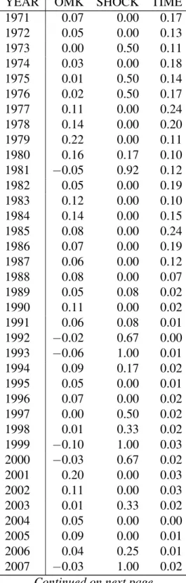
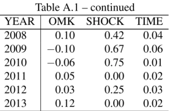
Table A.1 presents the annual means ofOM K,SHOCK, andT IM E. The table reveals that

OM Kdemonstrates non-monotonic variation in the time-series, consistent with fluctuations in the

degree of technology shock over time.SHOCK indicates the percent of months in each year that

1_{CPI data are available at: http://www.bls.gov/cpi/.}

are in the lowest quartile ofOM Kacross the sample, and ranges from 0 to 1. Interestingly, mean

SHOCK is at its highest in 1981, 1993, 1999, and 2007, years around which IBM introduced

the first PC, the World Wide Web was launched, Internet commerce expanded, and social media

became mainstream.3

To further validateOM K, I also obtained the annual wage growth statistics for Santa Clara and

San Mateo counties, two counties comprising the Silicon Valley, as a proxy for wage growth of

key talent.4 I use Silicon Valley wage growth as a proxy for the wage growth of key talent because the Silicon Valley has historically been known for its active technology entrepreneurship, and it

has a high density of engineers, researchers, and managers. I find that the average wage growth in

these two counties is negatively correlated with OM K (Pearson correlation of−0.36, p-value of 0.02), consistent withOM Kreflecting the market’s response to rising costs of key talent retention.

I also obtain the US aggregate annual percent wage growth data from the BEA for NAICS group

54, professional, scientific, and technical services. This category of business is likely to employ

professionals that would be considered key talent. Data are available from 1998-2013, and are

negatively correlated withOM K over that period (Pearson correlation of−0.44, p-value of 0.09), also consistent with OM K capturing the market’s response to the increased cost of retention of

key talent.

I also obtain technology book publishing data from Alexopoulos (2011) to determine variation

inOM K is correlated with the introduction of new technologies. Alexopoulos (2011) uses data

on technology book publications as a bottom-up measure of the introduction of new technologies.

However, this data is likely to lag the actual introduction of the new technology. Therefore, in

order to estimate the times of new technology introduction using this data, I calculate the annual

average percent growth of computer books and networking books over the periodt+ 1 to t+ 3

as a proxy for the degree of new technology introduction in year t. Higher future technology

3_{These examples are descriptive. Years for the introduction of the PC (1981) and World Wide Web (1992) are from}

Alexopoulos (2011).

book publications are an indication of the introduction of new technologies. Data are available to

calculate this measure from 1972-1994. Over this period, I find that future book publications are

negatively correlated withOM K (Pearson correlation of−0.45, p-value of 0.03), consistent with lower levels ofOM Kaligning with the introduction of new technologies.

T IM E demonstrates a significant downward trend, consistent with findings regarding the

di-minishing earnings-returns relation (Srivastava 2014; Lev and Zarowin 1999), but it also

demon-strates variation from year-to-year (Basu 1997). By year, the lowest values ofT IM Eare near zero

in 1992 and 2004 and the highest are around 0.24 in 1977 and 1985.

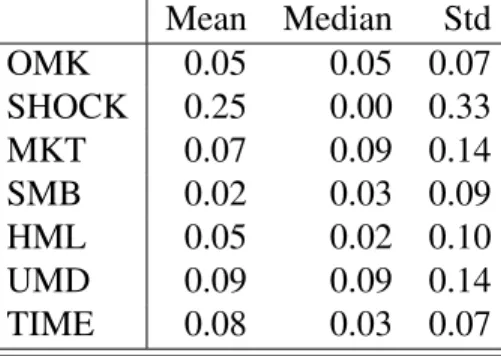
Table A.2 presents the means, medians, and standard deviation across all years for OM K,

SHOCK, M KT, SM B, HM L, U M D, andT IM E. The mean and median of OM K is 0.05,

consistent with the main finding in Eisfeldt and Papanikolaou (2013) that firms in the top quintile

ofOC have returns on average about 4.7% higher than those in the lowest quintile, indicating that

these firms are exposed to more systematic risk. AverageOM K is also in the range of returns of

the other factor portfolios.

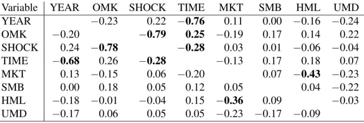
Table A.3 presents the correlations of the annual time-series variables. The negative

correla-tion betweenT IM Eand the calendar year,Y EAR, is significantly negative (Pearson (Spearman)

correlation =−0.76 (−0.68), p-value =<0.01 (<0.01)), consistent with the downward time trend documented in prior studies. No other variable demonstrates any significant time trend. The

corre-lation betweenSHOCK andT IM E is significant and negative (Pearson (Spearman) correlation

= −0.28 (−0.28), p-value = 0.07 (0.07)), consistent with periods of technology shock being as-sociated with lower earnings timeliness. The correlation between SHOCK and the other factor

portfolios is insignificant, suggesting that the effect captured bySHOCK is different from that

captured by other factors.

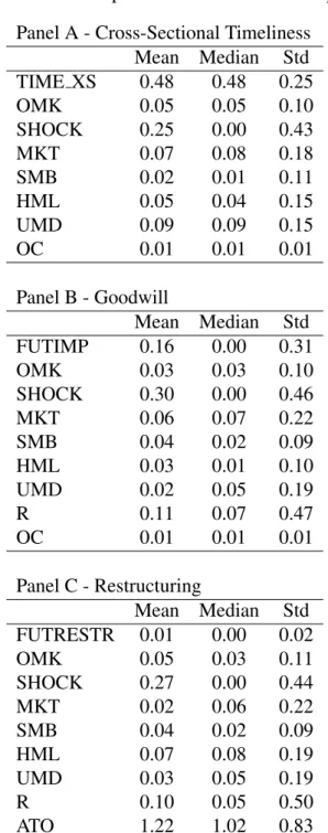
The descriptive statistics for the sample used in the estimation of equations (4.3) through 4.7 are

presented in Table A.4. Panel A presents the descriptive statistics for the sample used to perform

the additional tests of earnings timeliness. The mean ofT IM E XSis higher than the mean of the

two estimations of equation (4.2). Also, the explanatory power of the estimation may be higher

because the estimation is conducted within industry-year and portfolio-year groups, which relaxes

the assumption that all firms in a year have the same coefficients. The means of the time-series

variables have means similar to the aggregate averages presented in Table A.2.

Panel B presents descriptive statistics for the sample used to perform the goodwill tests. The

mean ofF U T IM P indicates that future impairments are on average about 16% of total goodwill,

but that the median is near zero. The summary statistics ofOM K, SHOCK, andOC are

gener-ally consistent with the statistics in the larger sample in panel A. The means and medians of the

factor returns appear different from those presented in Table A.2, reflecting the difference in the

time period of the sample, but remain in the 0.02 to 0.09 range of factor returns presented on Table

A.2.

Panel C presents descriptive statistics for the sample used to perform the restructuring tests.

The mean and median of F U T REST R indicate that the average future impairment charge is

about 1% of total assets, but that the median firm does not record any impairment charge. The

means and medians of the time-series variables are in the same range as those presented in Panels

CHAPTER 6: RESULTS

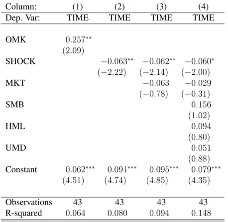
Table A.5 presents regression summary statistics for the estimation of equation (4.1) over the

43 year sample period. Column (1) usesOM Kas the measure of technology shock, and indicates

a positive coefficient forOM K (coefficient of 0.257, t-statistic of 2.09), consistent with

technol-ogy shocks being associated with lower levels of earnings timeliness, as measured by T IM E.

Columns (2) through (4) useSHOCK as the measure of technology shock, and include either no

controls (column (2)), market returns as a control (column (3)), or the full set of Fama and French

(1993) and Carhart (1997) factor returns as controls (column (4)). In all three columns, the

coef-ficient forSHOCK is significantly negative (coefficient between −0.060 and−0.063, t-statistic between −2.22 and −2.00). The results are in-line with the bi-variate correlations presented on table A.3, which indicate a significantly negative correlation between times of technology shock

and earnings timeliness. These results provide evidence consistent with hypothesis 1, that earnings

is less timely during times of technology shock. The magnitude of the coefficient suggests that

periods of technology shock demonstrate levels of timeliness that are about six percentage points

lower, all else equal. No other variable has a significant coefficient, consistent with correlations on

Table A.3.

Table A.6 presents regression summary statistics for theT IM E XS estimating equation (4.3)

includingOM Kas a measure of technology shock and including either no interaction withOC R

or controls (column (1)), the interaction with OC R and no controls (column (2)), or both the

interaction and controls (column (3)). The results in column (1) are consistent with the finding in

table A.5, that OM K has a positive association with earnings timeliness, measured in this case

by T IM E XS (coefficient of 0.243, t-statistic of 1.91). Column (2) and column (3) indicates

interaction between OM K and OC R (coefficient of −0.015 or −0.013, t-statistic of −5.38 or

−5.78). These results are consistent with hypothesis 1a, that the effect of technology shocks on earnings timeliness is increasing in the firm’s level of organizational capital. I interpret this as an

indication that organizational capital is a mediator by which technology shocks affect timeliness.

The coefficient on OC R is also negative and significant (coefficient of −0.015 or −0.013, t-statistic of −5.38 or −5.78), indicating that firms with higher levels of organizational capital on average have lower timeliness. The coefficients for the control variables are insignificant, with

the exception of M KT and U M D. The coefficient on M KT is significantly negative, which

is consistent with the notion that bad news is more effectively reflected in earnings than good

news. I have no interpretation for the significant coefficient onU M D. Untabulated results indicate

that using SHOCK as an indicator for technology shock instead of OM K provides the same

inferences, and that results are robust to the inclusion ofR, a measure of the firm’s idiosyncratic

returns.

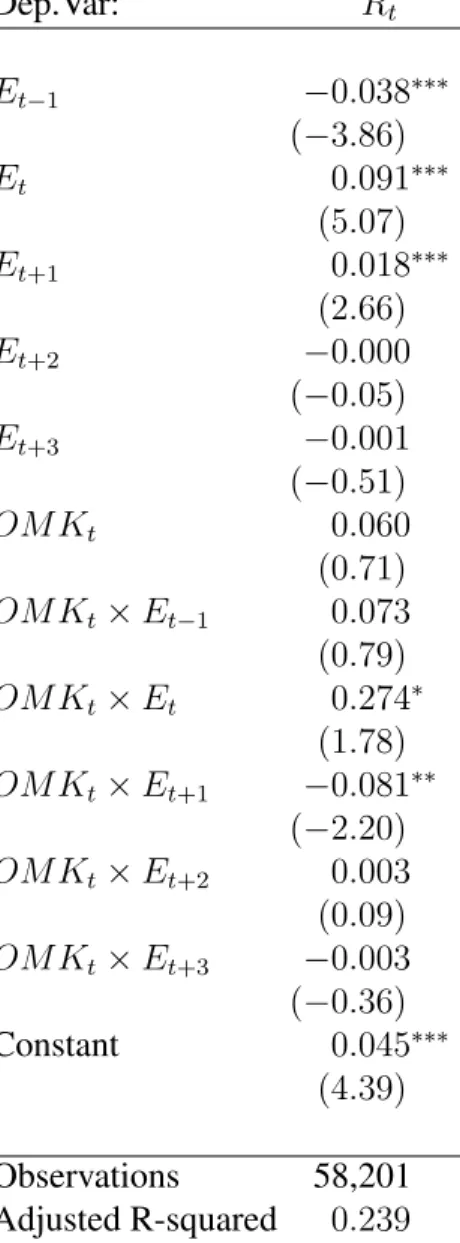
Table A.7 presents the regression summary statistics for the return estimating equation (4.4).

The coefficients on Et andEt+1 are positive, which is consistent with returns being reflected in

earnings contemporaneously or with a delay on average. The interaction termOM K ×Et has a

significantly positive coefficient (coefficient = 0.274, t-statistic = 1.78). Because lower returns to

OM K are consistent with a higher degree of technology shock, the positive coefficient is

inter-preted as current earnings being less associated with current returns during times of technology

shock. To the extent that current returns reflect the information revealed during the period, I

in-terpret this as an indication that current earnings captures less value-relevant information during

technology shocks. Also, the coefficient onOM K×Et+1 is negative and significant (coefficient

= −.081, t-statistic =−2.20). This is consistent with current returns being more associated with future expected earnings. I interpret this as an indication that current value-relevant information is

more likely to be reflected in future expected earnings during times of technology shock. I interpret

these coefficients together as an indication that periods of technology shock reveal information that

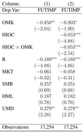
Column (1) of table A.8 presents regression summary statistics from the goodwill estimating

equation (4.5). Consistent with hypothesis 2, the coefficient onOM Kis significantly negative

(co-efficient =−0.850, t-statistic =−2.04). Because lower levels of OM K are consistent with more technology shock, this result suggests that periods of technology shock lead to higher goodwill

im-pairment charges, in line with the notion that technology shocks reduce the value of organizational

capital. This result provides an indication of how exogenous shocks to the value of intangible assets

can change the likelihood of a goodwill impairment charge appearing in earnings. The coefficient

onRis significantly negative, which is also consistent with expectations. Untabulated results

indi-cate that usingSHOCK as an indicator for technology shock instead ofOM Kprovides identical

inferences.

Column (2) of table A.8 presents regression summary statistics from the goodwill estimating

equation (4.6). Consistent with hypothesis 2a, the coefficient on the interaction of OM K and

HIOCis significantly negative (coefficient =−0.053, t-statistic =−2.54). This suggests that firms with higher levels of organizational capital in goodwill are more subject to the effects of technology

shocks on goodwill impairment. This effect is incremental to the main effects that technology

shocks and investment in organizational capital have on goodwill impairment, as indicated by the

significantly negative coefficients onOM K andHIOC.

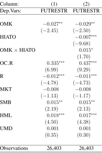
Column (1) of table A.9 presents regression summary statistics from the restructuring charge

estimation, equation (4.7). Consistent with hypothesis 3, the coefficient onOM K is significantly

negative (coefficient of−0.027, t-statistic of−2.45). Because lower levels ofOM Kindicate times of technology shock, this finding is consistent with technology shocks being associated with higher

and more frequent restructuring charges. This finding provides evidence that technology shocks

increase the attractiveness of new technology adoption, and provides insight as to how exogenous

shocks to the value of intangible investment can affect the likelihood of a firm incurring a

restruc-turing charge. The coefficient on R is significantly negative, also consistent with expectations.

Untabulated results indicate that usingSHOCK as an indicator for technology shock instead of

Column (2) of table A.9 presents regression summary statistics from the restructuring charge

estimation, equation (4.8). Consistent with hypothesis 3a, the coefficient on the interaction

be-tweenOM K andHIAT O is significantly positive (coefficient of 0.015, t-statistic of 1.70). This

result provides evidence that during times of technology shock, the increase in restructuring charges

is lower for firms with more efficient organizational capital. This effect is incremental to the main

effect that technology shocks have on increasing restructuring charges, as indicated by the negative

coefficient onOM K, and the effect that higher efficiency of organizational capital has on reducing

CHAPTER 7: CONCLUSION

This study investigates the effect that aggregate technology shocks have on the characteristics

of earnings. Eisfeldt and Papanikolaou (2013) suggests that technology shocks have two main

effects. First, they reduce shareholder’s value in organizational capital, and second, they increase

the likelihood of new technology adoption. Based on these effects, I generate my hypotheses. First,

I hypothesize that earnings reflects contemporaneous changes in value in a less timely manner

when technology shocks occur, particularly for firms with more organizational capital. Second, I

hypothesize that goodwill impairments increase subsequent to technology shocks, and particularly

for firms with more organizational capital in goodwill. Third, I hypothesize that restructuring

charges increase subsequent to technology shocks, and that more efficient firms will be less likely

to restructure after technology shocks. My tests provide evidence consistent with my hypotheses.

Findings from my study shed light on how the dynamics of the aggregate economy affect

the time-series and cross-sectional variation in the characteristics earnings. More specifically,

this study demonstrates one way in which investment in a specific intangible asset, organizational

APPENDIX A: TABLES

Table A.1: Aggregate Means by Year

YEAR OMK SHOCK TIME

1971 0.07 0.00 0.17

1972 0.05 0.00 0.13

1973 0.00 0.50 0.11

1974 0.03 0.00 0.18

1975 0.01 0.50 0.14

1976 0.02 0.50 0.17

1977 0.11 0.00 0.24

1978 0.14 0.00 0.20

1979 0.22 0.00 0.11

1980 0.16 0.17 0.10

1981 −0.05 0.92 0.12

1982 0.05 0.00 0.19

1983 0.12 0.00 0.10

1984 0.14 0.00 0.15

1985 0.08 0.00 0.24

1986 0.07 0.00 0.19

1987 0.06 0.00 0.12

1988 0.08 0.00 0.07

1989 0.05 0.08 0.02

1990 0.11 0.00 0.02

1991 0.06 0.08 0.01

1992 −0.02 0.67 0.00

1993 −0.06 1.00 0.01

1994 0.09 0.17 0.02

1995 0.05 0.00 0.01

1996 0.07 0.00 0.02

1997 0.00 0.50 0.02

1998 0.01 0.33 0.02

1999 −0.10 1.00 0.03

2000 −0.03 0.67 0.02

2001 0.20 0.00 0.03

2002 0.11 0.00 0.03

2003 0.01 0.33 0.02

2004 0.05 0.00 0.00

2005 0.09 0.00 0.01

2006 0.04 0.25 0.01

2007 −0.03 1.00 0.02