USING REGIONAL DATA SETS TO STUDY SOURCE TO SINK SEDIMENTARY PROCESSES
John R. Gunnell
A dissertation submitted to the faculty at the University of North Carolina at Chapel Hill in partial fulfillment of the requirements for the degree of Doctor of Philosophy in the Department
of Marine Sciences.
Chapel Hill 2016
iii ABSTRACT
John R. Gunnell: Using Regional Data Sets to Study Source to Sink Sedimentary Processes (Under the Direction of Brent McKee)
The study of sediment provenance, transport, and deposition encompasses a diverse set of geomorphological settings and processes. For a variety of reasons, “source to sink” sedimentary systems have historically been difficult to characterize due to operational limitations of the scientists studying them. Consequently, these systems are understood through the comparison of small-scale observational case studies. This lack of quantitative unity between studies has stymied attempts at building generalizable theory. The purpose of this dissertation is to
reevaluate some longstanding intuitions in the field of sedimentary geomorphology by taking a broader vantage and integrating observations from expansive regional scopes into unified frames of reference. This undertaking has revealed important insights about the behavior of several source to sink systems that would not have been noticeable if they were studied in a narrower context. An overview of these insights by chapter is as follows:
iv
Chapter 2: Despite the complex cascade of expected landscape responses to urbanization, suspended sediment yields of U.S. Piedmont streams consistently were an order of magnitude higher in watersheds with spatial indices of extensive population growth and urban development.
v
ACKNOWLEDGEMENTS
vi
TABLE OF CONTENTS
LIST OF TABLES ... ix
LIST OF FIGURES ...x
LIST OF ABBREVIATIONS AND SYMBOLS ... xiv
CHAPTER 1: A LARGE SCALE STUDY OF COASTAL WETLAND GEOMORPHOLOGICAL SETTINGS ...1
1.1: Introduction ...1
1.2: Methods ...2
1.2.1: Data Sources ...2
1.2.2: Data Extraction and Manipulation ...5
1.2.3: Statistical and Computational Methods ...7
1.3: Results ...8
1.3.1: Descriptive Statistics...8
1.3.2: Suspended Sediment Flux Regression and Validation ...12
1.3.3: Wetland Abundance Regression ...17
1.4: Discussion ...19
1.4.1: Estuarine vs. Fluvial Processes ...19
1.4.2: Knowledge Gaps in a Changing World ...22
1.5: Conclusions ...24
vii
CHAPTER 2: AN ANALYSIS OF FLUVIAL SUSPENDED
SEDIMENT RESPONSE TO URBANIZATION IN THE U.S. SOUTHERN PIEDMONT ...30
2.1: Introduction ...30
2.2: Methods ...32
2.2.1: Regional Description ...32
2.2.2: Gage Sites ...32
2.2.3: Fluvial Sediment Flux Estimation ...33
2.2.4: Spatial Analysis ...35
2.3: Results ...38
2.3.1: Sediment Flux Estimation Parameters ...38
2.3.2: Watershed Delineation Performance ...41
2.3.3: Spatial Characteristics between Sites ...42
2.3.4: Sediment Yield Comparisons ...45
2.4: Discussion ...47
2.4.1: Methodological Limitations ...47
2.4.2: Regional Differences ...48
2.5: Conclusions ...50
REFERENCES ...51
CHAPTER 3: A REVIEW OF MARSH SOIL PROPERTIES COMPARED TO MODELED EXPECTATIONS ...55
3.1: Introduction ...55
3.2: Methods ...56
3.2.1: Data Sources ...56
viii
3.2.3: Model Organization ...62
3.2.4: Modeling Primary Production ...64
3.2.5: Modeling Mortality and Decay ...63
3.2.6: Modeling Compaction and Accretion ...65
3.2.7: Model Comparison and Fitting ...68
3.3: Results ...69
3.3.1: Compilation Data ...69
3.3.2: Model Parameter Results ...73
3.3.3: Across Site Performance ...76
3.4: Discussion ...79
3.4.1: Failed Convergence ...79
3.4.2: Compression Error ...80
3.4.3: Recommendations for Future Research ...83
3.5: Conclusions ...84
REFERENCES ...85
APPENDIX A.1: STREAM GAGE SUMMARY ...92
APPENDIX A.2: SEDIMENT RATING CURVES ...94
ix
LIST OF TABLES
Table 1.1- Spatial Data Sources ...3
Table 1.2- Watershed Elevation Categories (Milliman and Syvitski 1992) ...6
Table 1.3- Bivariate Correlation ...9
Table 2.1- Changes in Land Cover (2001-2011) [% of Watershed Area] ...42
Table 3.1- Summary Statistics of Cores from the Literature ...59
Table 3.2- Tide Gage Information ...60
Table 3.3- Equations ...67
Table 3.4- Variables and Constants ...68
Table A.1.1- Gage Summary Table 1 ...92
Table A.1.2- Gage Summary Table 2 ...93
Table B.1- Core Summary Data from Literature ...146
Table B.2- Core Summary Data from Literature Continued1 ...147
x
LIST OF FIGURES
Figure 1.1- Terrain Variables ...4
Figure 1.2- Climate Variables Table ...5
Figure 1.3- Sediment Yield Descriptive Responses ...10
Figure 1.4- Marsh Width Descriptive Responses ...11
Figure 1.5- Diagnostic Charts for Regressions ...14
Figure 1.6- GAM Terms for Sediment Yield Regression ...15
Figure 1.7- Representativeness of the Suspended Sediment Estimate ...16
Figure 1.8- GAM Terms for Coastal Wetland Abundance ...18
Figure 2.1- Example of Sediment Rating Curve Analysis ...35
Figure 2.2- Spatial Datasets of Human Behavior ...37
Figure 2.3- Variation in Rating Curve Parameters ...40
Figure 2.4- Delineated Watersheds ...41
Figure 2.5- Mean within-Site Characteristics ...44
Figure 3.1- Cores and Spatial Datasets ...58
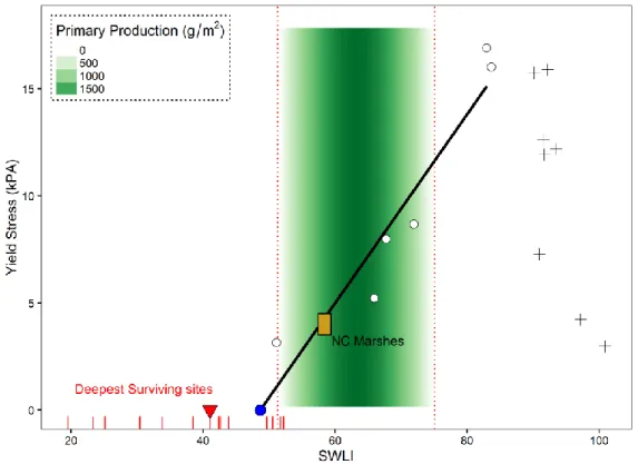
Figure 3.2- SWLI vs. Marsh Characteristics ...61
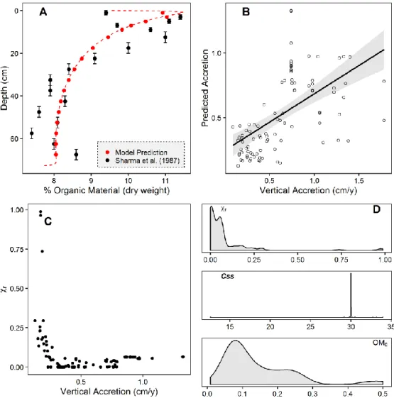
Figure 3.3- Factors Affecting Accretion ...71
Figure 3.4- Bivariate Soil Relationships ...72
Figure 3.5- Model Performance and Inferred Variables ...75
Figure 3.6- Systematic Model Errors ...78
Figure A.2.1-01673000: PAMUNKEY RIVER NEAR HANOVER, VA ...94
Figure A.2.2-02035000: JAMES RIVER AT CARTERSVILLE, VA ...95
Figure A.2.3-02041650: APPOMATTOX RIVER AT MATOACA, VA ...96
xi
Figure A.2.5-02085500: FLAT RIVER AT BAHAMA, NC ...98
Figure A.2.6-0208524090: MOUNTAIN CREEK AT SR1617 NR BAHAMA, NC ...99
Figure A.2.7-0208521324: LITTLE RIVER AT SR1461 NEAR ORANGE FACTORY, NC ...100
Figure A.2.8-0208650112: FLAT RIVER TRIB NR WILLARDVILLE, NC ...101
Figure A.2.9-0208524975: LITTLE R BL LITTLE R TRIB AT FAIRNTOSH, NC ...102
Figure A.2.10-02085000: ENO RIVER AT HILLSBOROUGH, NC ...103
Figure A.2.11-02096846: CANE CREEK NEAR ORANGE GROVE, NC ...104
Figure A.2.12-0208700780: LITTLE LICK CR AB SR1814 NR OAK GROVE, NC...105
Figure A.2.13-02087183: NEUSE RIVER NEAR FALLS, NC ...106
Figure A.2.14-02097464: MORGAN CREEK NEAR WHITE CROSS, NC ...107
Figure A.2.15-02097517: MORGAN CREEK NEAR CHAPEL HILL, NC ...108
Figure A.2.16-02116500: YADKIN RIVER AT YADKIN COLLEGE, NC ...109
Figure A.2.17-02096960: HAW RIVER NEAR BYNUM, NC ...110
Figure A.2.18-0209782609: WHITE OAK CR AT MOUTH NEAR GREEN LEVEL, NC ...111
Figure A.2.19-02087580: SWIFT CREEK NEAR APEX, NC ...112
Figure A.2.20-02087500: NEUSE RIVER NEAR CLAYTON, NC ...113
Figure A.2.21-0214266000: MCDOWELL CREEK NR CHARLOTTE, NC (CSW10) ...114
Figure A.2.22-02124692: GOOSE CR AT FAIRVIEW, NC ...115
Figure A.2.23-02126000: ROCKY RIVER NEAR NORWOOD, NC ...116
Figure A.2.24-02331600: CHATTAHOOCHEE RIVER NEAR CORNELIA, GA...117
Figure A.2.25-02333500: CHESTATEE RIVER NEAR DAHLONEGA, GA ...118
Figure A.2.26-02334480: RICHLAND CREEK AT SUWANEE DAM ROAD, NEAR BUFORD,GA ...119
xii
Figure A.2.28-02217274: WHEELER CREEK AT BILL
CHEEK ROAD, NEAR AUBURN, GA ...121 Figure A.2.29-02334885: SUWANEE CREEK AT SUWANEE, GA ...122 Figure A.2.30-02218565: APALACHEE RIVER AT FENCE
ROAD, NEAR DACULA, GA ...123 Figure A.2.31-02335350: CROOKED CREEK NEAR NORCROSS, GA...124 Figure A.2.32-02335870: SOPE CREEK NEAR MARIETTA, GA...125 Figure A.2.33-02208150: ALCOVY RIVER AT NEW
HOPE ROAD, NEAR GRAYSON, GA ...126 Figure A.2.34-02336030: N.F. PEACHTREE CREEK
AT GRAVES RD, NR DORAVILLE,GA ...127 Figure A.2.35-02336360: NANCY CREEK AT RICKENBACKER
DRIVE, AT ATLANTA, GA ...128 Figure A.2.36-02336410: NANCY CREEK AT WEST WESLEY
ROAD, AT ATLANTA, GA ...129 Figure A.2.37-02336120: N.F. PEACHTREE CREEK,
BUFORD HWY, NEAR ATLANTA, GA ...130 Figure A.2.38-02207400: BRUSHY FORK CREEK AT
BEAVER ROAD, NR LOGANVILLE,GA ...131 Figure A.2.39-02336300: PEACHTREE CREEK AT ATLANTA, GA...132 Figure A.2.40-02207385: BIG HAYNES CREEK AT LENORA
ROAD, NR SNELLVILLE, GA ...133 Figure A.2.41-02336240: S.F. PEACHTREE CREEK JOHNSON RD,
NEAR ATLANTA, GA ...134 Figure A.2.42-02336526: PROCTOR CREEK AT JACKSON
PARKWAY, AT ATLANTA, GA ...135 Figure A.2.43-02207185: NO BUSINESS CREEK AT LEE
ROAD, BELOW SNELLVILLE,GA ...136 Figure A.2.44-02207120: YELLOW RIVER AT GA 124, NEAR LITHONIA, GA ...137 Figure A.2.45-02207220: YELLOW RIVER AT PLEASANT
xiii
Figure A.2.46-02203655: SOUTH RIVER AT FORREST
PARK ROAD, AT ATLANTA, GA...139 Figure A.2.47-02207335: YELLOW RIVER AT GEES
MILL ROAD, NEAR MILSTEAD, GA...140 Figure A.2.48-02337500: SNAKE CREEK NEAR WHITESBURG, GA ...141 Figure A.2.49-02338000: CHATTAHOOCHEE RIVER NEAR WHITESBURG, GA...142 Figure A.2.50-02338523: HILLABAHATCHEE CREEK
xiv
LIST OF ABBREVIATIONS AND SYMBOLS
Bag Total aboveground biomass
bbg Belowground biomass within a sediment cohort Bbg Total belowground biomass
BD Dry bulk density
Bp Annual peak value of total aboveground biomass Cr Recompression coefficient
Cc Compression coefficient
Cs Suspended sediment concentration
Css Input variable for marsh sedimentation model parameterizing differences in sediment availability
DN Digital Number
Dni Depth below mean high water at the North Inlet, SC E Duan’s smearing coefficient
e Void ratio of a sediment cohort e1 Reference void ratio at 1kPa ETOPO1 Global 1’ digital elevation model
GAM Generalized Additive Model, a nonlinear regression method GCV Generalized Cross Validation statistic
Gs Specific gravity of particulate matter HAT Highest astronomical tide
IQR Interquartile range
xv LAT Lowest astronomical tide
Mag Total mortality of aboveground biomass
m Mortality of belowground biomass within a sediment cohort MD Dry mineral density
MHW Mean high water
NLCD National Land Cover Database NWIS National Water Information System OMD Dry organic matter density
OM0 Input variable for marsh sedimentation model parameterizing the proportion of incoming sediment comprised of refractory organic material
Q(t) Fluvial discharge as a function of time
Qs(t) Suspended sediment flux as a function of time
r(y) Sediment rating curve model residuals as a function of year
RMSE Root mean square error of residuals between predicted and measured values rSLR The rate of relative sea level rise
SWLI Standardized water level index
Stn-30p 30’ Global delineated watershed data set
T Temperature
Tni Temperature at the North Inlet, SC
%OM Percent organic material of dry sediment based on loss on ignition
γz Coefficient modifying the rate that belowground biomass decreases with respect to depth
η0 Initial elevation of first sediment deposit in the marsh sedimentation model μ Coefficient modifying the rate that organic matter decay decreases with respect to
depth
xvi ρwet The wet particle density of soil material
σb Coefficient modifying peak total annual aboveground biomass based on deviation from a reference temperature
σk Coefficient modifying rates of organic matter decay based on based on deviation from a reference temperature
σ’ Effective compressive stress above a sediment cohort σ’y Yield stress of a sediment cohort
τ Kendell’s nonparametric correlation coefficient
1
CHAPTER 1: A LARGE SCALE STUDY OF COASTAL WETLAND GEOMORPHOLOGICAL SETTINGS
1.1 Introduction
Long valued for their ecosystem services(Costanza et al., 1997), salt marshes are more recently noted for their importance in the global carbon cycle (Nellemann et al., 2009; Chmura et al., 2003) and carbon sequestration (Grimsditch et al., 2012; Pendleton et al., 2012). This is because these emergent coastal wetlands experience significant primary production, rapid sedimentation, and slow carbon remineralization (Duarte et al., 2005). Despite this growing interest, no global inventory of salt marsh area exists (Hopkinson et al., 2012). Global
anthropogenic change also threatens wetland survival in a variety of climate conditions (Kirwan et al., 2010; Kirwan and Mudd 2012). Therefore, the abundance of coastal wetlands is uncertain for both the present and future. The goal of this exploratory analysis is to make a tentative estimate of how the coastal marsh’s geomorphological setting influences its regional abundance using large scale datasets. This will function as an evaluation of current theory on marsh
geomorphology and may guide future endeavors to predict a global inventory of coastal wetland abundance.
A rich literature of environmental case studies has informed us that marsh erosion and sedimentation vary due to differences in ambient wave energy (Fagherazzi et al., 2006), channel proximity(Cahoon and Reed 1995), marsh-table elevation (Allen 2000), and primary
2
Gunnell et al., 2013; Day et al., 2011; Krull and Craft 2009), and extrapolations from
mechanistic models (Fagherazzi et al., 2012). Due to a historical paucity of continental datasets, it is not certain how these various factors interact to influence large scale wetland predominance.
Until the continental-scale geomorphological settings of coastal wetlands are measured and compared to inventories, we can’t claim that we understand the emergent consequences of the processes dictating marsh behavior. We have an educated expectation that marshes should predominate in systems with high accommodation space, low energy, and with relatively high suspended sediment concentrations. In this study, we have gathered datasets that will act as indices for those features and compared them to marsh abundance.
1.2 Methods
1.2.1 Data Sources
Spatial covariates from global data sets were compared to the abundance of “Estuarine and Marine Intertidal Wetlands” reported in the U.S. National Wetlands Inventory (Table 1). According to the wetland inventory, this category includes “both vegetated and non-vegetated brackish and saltwater marsh, shrubs, beach, bar, shoal, or flat”. It is our expectation that this will largely be comprised of marshland and sedimentary structures that behave similarly to marshes.
Terrain attributes (Fig. 1.1) include a high resolution global shoreline (Wessel and Smith 1996), the Stn-30p global delineated watersheds (Vörösmarty and Fekete 2011), estimates of sediment flux to the ocean (Milliman and Farnsworth 2012), and the ETOPO1 bedrock
3
maps are available and have been used in other global sediment flux measurements (Syvitski and Kettner 2011), ETOPO1’s inclusion of bathymetry means that river mouth and estuarine terrain analysis can include subaqueous topography. Relief was measured using the “roughness” index calculated using the ‘terrain’ function in the R raster package (Hijmans 2014). This value is the maximum range of elevations (meters) within the 8-cell neighborhood of the point being
measured.
Table 1.1-Spatial Data Sources:
Feature type (resolution) reference
Global Shoreline Line (~1 km) (Wessel and Smith 1996) Sediment Yield Point (Milliman and Farnsworth 2012) Watersheds Polygon (30’) (Vörösmarty and Fekete 2011) Topography Raster (1’) (Amante and Eakins 2009) Temp/Precip Raster (1.4°) (NCAR-GIS-Program 2012) Wave Energy Raster (30’) (Tolman 2009)
M2 Tidal Range Raster (15’) (Ray 1999)
Wetland Area Polygon (~15 m) (U.S. Fish and Wildlife Service 2016)
Climate variables (Fig. 1.2) include modeled surface temperature and total precipitation (NCAR-GIS-Program 2012), a modeled M2 tidal range (Ray 1990), and wave energy density derived from modeled significant wave heights (Tolman 2009). Surface Temperature and Total Precipitation datasets are monthly average projections for the historical period ranging from 1979 to 1999 (NCAR-GIS-Program 2012) on a 1.4 degree grid. These 20 year hindcasts were averaged within each cell before being projected to a final raster.
4
wave period (T): E = .5H2T. The final value reported is the mean of all time steps at each point. This is a qualitative measure of wave energy nearshore, because there is no accounting for bathymetric effects or wave diffraction.
Figure 1.1-Terrain Variables:
5
Figure 1.2-Climate Variables:
A: Average surface temperature from 1979-1999. Shoreline added for visualization. B: Average annual precipitation 1979-1999. Shoreline added for visualization. C: M2 (semi-diurnal
contribution) tidal constituent. D: Offshore wave energy density. 1.2.2 Data Extraction and Manipulation
6
area (1000s km2), and “elevation category” (an ordered factor in the table) were taken from the Milliman and Farnsworth global river database and were used in a regression analysis to project sediment flux at unmeasured locations.
Although the full Milliman and Farnsworth database is larger, this selection comprised complete cases of all attributes of interest. Where “Pre Dam” suspended sediment flux values were supplied, they were substituted for this analysis. Categorical elevations (as used in Milliman and Syvitski 1992 and others; Table 1.2) were chosen over “Maximum Elevation” measurements due to the low resolution of reported values. In many cases, reported elevations were simply the cutoff values for the categories. Additionally, “Coastal Plain” and “Lowland” categories were combined for regression due to the paucity of “Coastal Plain” samples. The data set also reports latitudes and longitudes for river mouths. These locations were used to extract underlying raster values for precipitation, temperature, and roughness from corresponding datasets described earlier.
Table 1.2 Watershed Elevation Categories (Milliman and Syvitski 1992)-
Category Maximum
Elevation
# Samples
Coastal Plain < 100 m 19
Lowland 100 - 500 m 105
Upland 500 - 1000 m 159
Mountain 1000 - 3000 m 402
High Mountain > 3000 m 81
7
polygon, then categorizing the elevation value using the previously mentioned cut off values. Basin areas were reported in the original dataset (Vörösmarty and Fekete 2011), and additional attributes (temperature, precipitation, and roughness) were extracted to the spatial points of the river mouths. These assembled predictors were then used as input data for a regression model based on the Milliman and Farnsworth data.
Wetland area and spatial covariates were extracted to 2° square spatial bins intersecting with the shoreline. The bins and all spatial fields were projected to Mollweide equal area before extraction. Values collected for the climate variables and roughness are binned averages. The value for wetland area is total intersecting area. Total transported sediment within each bin is the sum of predicted values found in exorheic Stn-30p river mouth points intersecting with each bin. The length of shoreline is the sum of the Euclidean distances between consecutive vertices of the shoreline segment intersecting with the bin. It is uncertain how this estimated length will be impacted by resolution effects (Mandelbrot 1967). Wetland area and total suspended sediment values were both divided by shoreline length within each bin to normalize for differences in coverage between bins. For this study, the normalized wetland area is referred to as “Marsh Width”.
1.2.3 Statistical and Computational Methods
8
spline, while a tensor smooth is a surface. These surface interaction terms (e.g. Fig. 1.6A,B; Fig. 1.8A,B,C) are not simply sums of the two terms’ influence on the model. Instead, they
demonstrate the unique relative impact on the model each potential pairing would have on the outcome.
Optimal model selection was selected based on minimum AIC and with the further constraint that all regressor terms be statistically significant based on Wald like tests (Wood 2006). The optimal selected model for sediment yield was used to make worldwide predictions of sediment flux to the ocean using river attributes of simulated watersheds (Stn-30p). These predicted values were used both to determine regional sediment yields adjacent to estuaries of interest, as well as to make a prediction of global cumulative sediment flux
All statistical and computational work was performed with the R statistical computing language v. 3.3.0 (R Core Team 2016). Geospatial operations were carried out using the sp, maptools, rgdal, and raster packages (Pebesma and Bivand 2005; Bivand et al., 2013; Bivand and Lewin-Koh 2014; Bivand et al., 2014; Hijmans 2014).
1.3 Results
1.3.1 Descriptive Statistics
9
A measurement of bivariate correlation using the non-parametric Kendall’s τ coefficient (Table 1.3) shows statistically significant relationships between marsh width and all spatial covariates except the M2 tidal constituent and shoreline-normalized annual sediment flux. Results of the sediment flux projection are in the next section.
Suspended sediment yield measurements in the 766 Milliman and Farnsworth river mouths showed statistically significant correlations with all covariates. In most cases,
correlation values, though statistically significant, were relatively modest in their magnitudes. Increases in river mouth roughness were correlated with higher sediment yields, but maximum elevation category also was related to increases in yield (Fig. 1.3A). Since maximum elevation can be far from the mouth, this demonstrates that fluvial sediment flux to the ocean is a product of both local and regional processes.
Table 1.3-Bivariate Correlation:
Marsh Width Sediment Yield
τ p τ p
Area - - -0.26 < .001
Temperature 0.15 < .05 0.2 < .001 Precipitation 0.12 < .05 0.1 < .001 Roughness -0.34 < .001 0.17 < .001
M2 0.015 n.s. - -
Wave Energy -0.2 < .001 - -
Sediment/Shore 0.08 n.s. - -
10
Figure 1.3-Sediment Yield Descriptive Responses:
A: A box and whisker plot of suspended sediment yield vs. elevation category using the categories from table 1.2 with coastal plain and lowland included in the same category. B-E:
11
Figure 1.4-Marsh Width Descriptive Responses:
12
1.3.2 Suspended Sediment Flux Regression and Validation
The optimal regression model for sediment yield was the sum of three smoothed terms and one constant term:
E
(
Yield
)=
f
(
Area
)+
f
(
Roughness
)+
f
(
Precip
,
Temp
)+
f
(
lat
,
long
)+
Elevation
The regression has an adjusted r2 of .6, shows normal residual errors (Fig. 1.5B) and a consistently proportionate relationship with known values (Fig. 1.5A). The interaction of Temperature and Precipitation was parameterized as a tensor spline with a cubic regression spline basis. Area and Roughness terms had cubic shrinkage spline bases, while Elevation classification was parameterized with an ordinal factor. To model spatial autocorrelation not captured by the other features, a thin plate regression spline depending on latitude and longitude was added.
As with other linear models, the predicted value is based on the sum of its terms. Instead of constant slopes, however, the effect of each variable on the prediction varies depending on its value. Since sediment yield was log-transformed for the regression, the value of each additive term will not be immediately intuitive. Looking at each smooth term’s contribution to the predicted value of sediment yield (Fig. 1.6), consider its relative influence on the prediction and whether it adds to or subtracts from the prediction. The contributions of basin area and
roughness are almost linear (Fig. 1.6C,D), and follow an intuitive pattern that parallels the actual trends in the data (Fig. 1.3B,E).
13
(Fig. 1.6B) shows higher term values along the Pacific Rim and lower values around the Atlantic, possibly capturing tectonic effects.
Sampling coverage is especially important when extrapolating from the model. For instance, there are very few points in regions of high precipitation but low temperature (Fig. 1.6A), possibly leading the model to predict unreasonably high values for that type of climate. Since the suspended sediment regression model is being used to generate data at unmeasured sites for this study, its representativeness needed to be evaluated. The feature space of the river mouths from Stn-30p and the Milliman and Farnsworth data set is shown in a principal
components analysis (Fig. 1.7C) where the first two principal components explain the majority of the variance. The convex hull (in grey) is a region containing all the points from the Milliman and Farnsworth data set, while the cloud of points represents the nearly 6000 river mouths of Stn-30p. Two point clouds (red and blue) largely stand outside this convex hull, showing that the combination of their attributes are especially distinctive from the features represented in the training data.
Points from both clouds have the capacity to show high coefficients of variation in their estimated values for sediment yield (Fig. 1.7A), because they are in a region of the regression with broad confidence intervals. Spatially (Fig. 1.7B), the two regions largely line up with arctic watersheds (blue) and equatorial islands (red). Looking at the PC loadings (Fig. 1.7C), these equatorial river mouths have low basin area, high temperature, high precipitation, and high roughness. Since they stand at the extreme boundaries of several additive terms in the
14
highest estimates of suspended sediment yield are removed from the prediction dataset, and our predictions are refined to exorheic basins, the sediment global flux estimate is comparable to others in the literature (Fig. 1.7D).
Figure 1.5-Diagnostic Charts for Regressions:
A: Actual yield measurements from Milliman and Farnsworth 2012 vs. predicted yields vs. regression. 1:1 values are along the black line. B: Histogram showing the distribution of predicted log(Yield) – log(Yield). The depended variable was transformed for regression. This is why the scale is different. C: Actual values of marsh width vs. predicted values using
regression. 1:1 is represented by the black line. D: Histogram showing the distribution of width residuals after predicted and measured values were transformed using the same Box-Cox
15
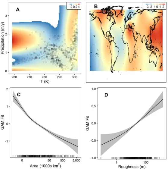
Figure 1.6-GAM Terms for Sediment Yield Regression:
A: The Temperature & Precipitation interaction term. Legend values (like ‘GAM Fit’ for C and D) are relative addition or subtraction to the predicted value of sediment yield. Points are the Milliman and Farnsworth river mouths used as training data. B: Spatial interaction term. Legend values follow the same rules. Shorelines were added for visualization purposes. C: Basin area vs. GAM term value. The rugplot shows the distribution of values in the training data. D:
16
Figure 1.7-Representativeness of the Suspended Sediment Estimate:
A: Coefficient of variation for each estimate of suspended sediment yield vs. the estimated value of Yield. Colored points are the same as in B and C. B: Spatial distribution of highlighted points. C: Principal components analysis of both Milliman and Farnsworth 2012 points and the Stn-30p delineated river mouths based on extracted features. A convex hull contains the Milliman and Farnsworth points. Stn-30p points standing largely outside this region in the feature space were delineated using arbitrary values along the first and second principal
17 1.3.3 Wetland Abundance Regression
The optimal regression model for marsh width was the sum of four smoothed terms:
E
(
Width
)=
f
(
Waves, TSS
)+
f
(
Roughness, M2
)+
f
(
Precip
,
Temp
)+
f
(45 – abs(
lat
))
The regression has an adjusted r2 of .58 with normal residual errors (Fig. 1.5D) and is in consistent proportion with known values (Fig. 1.5C). All three interaction terms were parameterized as a tensor spline with a cubic regression spline basis. The latitude term has a cubic shrinkage spline basis, and is meant to parameterize distance from the temperate region.
The width of coastal wetlands, as previously stated, is a shore-length normalized term for wetland abundance. This regression model of width was the most effective at explaining
variation out of a set of other candidate regression models which tested the ambient features as individual smooths and as different sets of interactions. Marsh width’s strong bivariate trends with respect to wave energy and roughness (Table 1.3) manifest themselves in the trend surfaces of their interaction terms (Fig. 1.8B,C), with consistently decreasing contributions to marsh width as their values increase. Shore-length normalized flux of terrestrial suspended sediment supply to the ocean, despite lacking significant bivariate correlation with marsh width (Table 1.3), apparently contributes to marsh width when present above a threshold quantity (Fig. 1.8C), but decreases in its contribution in a varying manner with respect to wave energy climate.
It is important to note that each term, while statistically significant, does not necessarily indicate substantial magnitudes of influence from each morphological parameter. M2 tidal component, for instance, does not exert a substantial change on its interaction term with
Roughness except at relatively high magnitudes (Fig. 1.8B). Furthermore, interactions between features, while suggestive of interactions on the landscape-level, do not guarantee
18
Figure 1.8-GAM Terms for Coastal Wetland Abundance:
Displayed is the variation in the relative contribution of each GAM term to wetland abundance if all other terms were held constant. Individual points are the values from the gridded coastlines containing National Wetlands Inventory values. A: GAM interaction term for Temperature & Precipitation. B: M2 & Roughness C: Wave energy density & Annual terrestrial sediment flux to the ocean normalized by shoreline length D: Distance from the nearest 45th parallel
19
trends within the interaction term between temperature and precipitation (Fig. 1.8A), indicating that collinearity with latitude overwrites the effect of explicit climate variables on the regression model.
1.4 Discussion
The lack of pronounced correlations between wetland abundance and most
geomorphological features indicates that wetlands exist and persist under a gradual continuum of influences. Furthermore, the apparent interactions between variables demonstrate the complexity of the system. Based on bivariate responses (Table 1.3), the strongest individual covariates are roughness and wave energy density. If we take a broader interpretation of what these covariates signify, roughness largely measures the proximity of the shoreline to the shelf break, and is an indicator of accommodation space. Wave energy density measures the potential wave energy in the absence of fetch limitation and bottom drag. These two features represent a shoreline’s capacity to store sediment and its potential erosional climate respectively. In addition to latitude, these two variables have a much larger apparent influence on wetland abundance than fluvial sediment availability. Despite each spatial feature’s subtle influence, it is clear that processes and features local to the estuary have the majority of apparent influence on wetland abundance. 1.4.1 Estuarine vs. Fluvial Processes
20
estuarine interface. The results from this large scale study imply a preeminence of local geomorphological processes in determining cumulative coastal wetland inventories.
The influence of local geomorphology on large scale sediment transport has long been apparent in continental systems. The importance of river mouth relief and climate-related erosion explains the exceptional sediment fluxes to the ocean in the small rivers of the East Indies (Milliman et al., 1999). On the other end of the size spectrum, it also explains the decline in sediment flux over the Amazon River’s course. Sediment flux from the Andes outweighs sediment flux in the lower river at Obidos more than twofold (Aalto et al., 2006; Dunne et al., 1998), because the lower river has lower relief and therefore has less stream power. The fluvial sediment flux estimates derived in this study demonstrate the same significance of climate and topography at the rivers’ mouths in hundreds of other locations all over the world. This study takes that intuition derived from terrestrial systems another step further downriver to demonstrate the importance of ambient coastal processes on dictating wetland abundance.
Past research in salt marshes has shown that sediment availability is certainly a factor in marsh accretion and expansion. New marshes frequently are structures resulting from recent sediment accumulation (Krull and Craft 2009; Mattheus et al., 2009; Cahoon et al., 2011), often built through sedimentary infilling of accommodation spaces such as estuaries (Kirwan et al., 2011) or crevasse splays(Cahoon et al., 2011). Accretion accelerates before the marsh forms, eventually producing an emergent sandbar or mudflat that is colonized by marsh grasses
(Gunnell et al., 2013; Krull and Craft 2009). This rapid accretion continues through the marsh’s incipience until it reaches a mature elevation (Pethick 1981).
21
interaction between fluvial sediment flux and wave energy (Fig. 1.8C) suggests that there must be some threshold quantity of sediment available before it contributes to wetland abundance, but below that threshold and at moderate wave energies, sediment availability has no apparent effect on wetland abundance. The processes sustaining marshes are not necessarily the same ones that built the marsh in the first place, which may explain this ambivalent result across so many sites. Sediment-starved regions that previously were sediment-rich can host marshes that maintain themselves through vegetative accretion (Nyman et al., 2006). In the absence of extensive erosion, it is only due to prolonged sediment starvation and rapid sea level rise that these wetlands eventually disappear due to subsidence and vegetation die-off (Syvitski et al., 2009; Day et al., 2011). Consequently, there is an indeterminate lag period between a marsh’s birth and demise regardless of sediment availability.
Higher wave energy environments demonstrate a more intuitive relationship of erosion and sedimentation offsetting each other (Fig. 1.8C). At higher sediment availabilities, increases in wave energy lead to less pronounced positive influence on wetland abundance. This may corroborate observations that over the course of marsh ontogeny, accretion rates are dependent on the effective shear stress on estuarine bottom sediments, strongly determining whether an emergent mudflat forms (Fagherazzi et al., 2006; Gunnell et al., 2013). At sites with lower incoming sediment and high wave energies, abundance is negatively affected.
22
makes intuitive sense. The tide’s capacity to redistribute sediments retained in the estuary is rendered moot in a high roughness estuary that doesn’t have the capacity to retain sediment. This interaction demonstrates the importance of long term estuarine sedimentary processes in maintaining wetland abundance. If terrestrial sediment supply were the overwhelmingly
dominant means of sustaining sediment concentrations in estuarine waters, this interaction would not be a significant factor.
1.4.2 Knowledge Gaps in a Changing World
The importance of climate on coastal wetland abundance appears to be the most equivocal of the regression components (Fig. 1.8A). The collinearity of the climate variables with the distance from the temperate zone (Fig. 1.8D) means that the structure of the temperature vs. precipitation interaction is harder to interpret. The positive effect on abundance presented by high temperature and high precipitation mirrors the same interaction shown in the sediment yield regression, where wet tropical rivers have high sediment yields. Perhaps this is a remnant of the influence of sediment availability. Negative influence at high precipitation sites of intermediate temperatures suggest that stormy temperate climates are connected to decreased abundance.
23
either because the datasets don’t yet exist, or the processes of interest haven’t quite happened yet.
This study appears to demonstrate that fluvial sediment flux to the ocean has a nuanced effect on coastal wetland abundance. The combination of extensive erosion and impoundment within the basins of major rivers has led to extreme historical variation in sediment flux (Syvitski and Kettner 2011; Syvitski and Milliman 2007). Smaller coastal rivers (100 and 3000 km2 in basin area), despite making up ~94% of all individual rivers that drain into the ocean (Milliman and Farnsworth 2011), are not well-represented in the global data set (e.g. “Coastal Plain” rivers in Table 1.2). How these smaller rivers interact with the estuarine system and influence the available reservoir of sediment is unmeasured. Their very existence lies outside the resolution of the delineated watersheds we used in this study.
Climatological consequences such as accelerated relative sea level rise are expected to affect wetland abundance (Kirwan et al., 2010), but their consequence can’t be measured using these contemporary data sets. Similarly, the ecological effect of competition between mangrove and marsh ecosystems can’t be observed using U.S. inventories due to the very small
contemporary overlap in geographic range (Giri et al., 2010). Changes in sediment supply in the arctic regions due to climate change can’t reliably be predicted with the current global sediment data set either. This is partly because the transformation those landscapes will experience has not occurred since the last ice age ended, and naturally has not been measured. If arctic
watersheds behaved similarly to other watersheds, they still would not be reliably estimated with these methods because the arctic region stands outside the feature-space of sites that have
24
scale consequences of global climate change on sediment flux to the oceans or wetland inventories because the coming changes are unique and the existing datasets are sparse.
1.5 Conclusions
Perhaps the most important insights gleaned over the course of this study were with respect to terrestrial sediment flux to the global oceans. Vast regions of the world’s oceans have contributing watersheds that stand outside the geomorphologically relevant feature-space of currently measured watersheds. Although these regions generally fail to intersect with the coastal United States, this lack of baseline characterization of contemporary sediment flux calls into question our capacity to predict sediment supply to the world’s oceans in both the present and future.
The second important observation with respect to terrestrial sediment flux was its weak connection to wetland abundance along U.S. coastlines. The addition of terrestrial sediment only leads to increases in marsh abundance when it is present in large quantities. Vertical accretion properties particular to marsh systems as well as the role of roughness and tidal forcing to redistribute sediment within an existing reservoir may both play a larger part in sustaining marsh sedimentation over longer timescales.
Due to the nature of global change, it is impossible to predict many of the impacts on this system using this manner of study. In a consistent climate and sea level rise scenario, the
25
REFERENCES
Aalto, R., T. Dunne, and J.L. Guyot. "Geomorphic controls on Andean denudation rates." The Journal of Geology 114.1 (2006): 85-99.
Allen, J. Morphodynamics of Holocene Salt marshes: a review sketch from the Atlantic and Southern North Sea coasts of Europe. Quaternary Sci. Rev. 19, 1839–1840 (2000). Amante, C., and B.W. Eakins. 2009. ETOPO1 1 Arc-Minute Global Relief Model: Procedures,
Data Sources and Analysis. NOAA Technical Memorandum NESDIS NGDC-24. National Geophysical Data Center, NOAA. http://dx.doi.org/10.7289/V5C8276M/. Bivand, R.S., E. Pebesma, and V. Gomez-Rubio. 2013. Applied Spatial Data Analysis with R,
Second Edition. Springer, NY. http://www.asdar-book.org/.
Bivand, R., and N. Lewin-Koh. 2014. Maptools: Tools for Reading and Handling Spatial Objects. http://CRAN.R-project.org/package=maptools.
Bivand, R., T. Keitt, and B. Rowlingson. 2014. Rgdal: Bindings for the Geospatial Data Abstraction Library. http://CRAN.R-project.org/package=rgdal.
Brown, M. 2012. “Marine Data Literacy : Providing Instruction for Handling (Managing, Converting, Analyzing and Displaying) Oceanographic Station Data, Marine
Meteorological Data, GIS-Compatible Marine and Coastal Data, and Mapped Remote Sensing Imagery.” http://www.marinedataliteracy.org/grids/360_to_180.htm.
Cahoon, D. R. and D.J. Reed. Relationships among marsh surface topography, hydroperiod, and soil accretion in a deteriorating Louisiana salt marsh. J. Coastal Res. 11, 357–369 (1995). Cahoon, D. R., D.A. White, and J.C. Lynch. Sediment infilling and wetland formation dynamics
in an active crevasse splay of the Mississippi River delta. Geomorphology 131, 57–68 (2011).
Canuel, E. A., C.S. Martens, and L.K. Benninger. "Seasonal variations in 7Be activity in the sediments of Cape Lookout Bight, North Carolina." Geochimica et Cosmochimica Acta 54.1 (1990): 237-245.
Chmura, G. and S. Anisfeld. Global carbon sequestration in tidal, saline wetland soils. Global Biogeochem. Cy. 17, (2003).
Corbett, D.R., B. McKee, and D. Duncan. "An evaluation of mobile mud dynamics in the Mississippi River deltaic region." Marine Geology 209.1 (2004): 91-112.
26
Dahl, T.E. 2011. Status and trends of wetlands in the conterminous United States 2004 to 2009.U.S. Department of the Interior; Fish and Wildlife Service, Washington, D.C. 108 pp.
Day, J. W. et al. Vegetation death and rapid loss of surface elevation in two contrasting
Mississippi delta salt marshes: The role of sedimentation, autocompaction and sea-level rise. Ecol. Eng. 37, 229–240 (2011).
Duarte, C., J.J. Middelburg, and N. Caraco. Major role of marine vegetation on the oceanic carbon cycle. Biogeosciences 2, 1–8 (2005).
Dunne, T., et al. "Exchanges of sediment between the flood plain and channel of the Amazon River in Brazil." Geological Society of America Bulletin 110.4 (1998): 450-467. Dürr, H. H., and G.G. Laruelle. 2011. “Global Coastal Typology.” Geotypes.net.
http://geotypes.net/downloads.html.
Dürr, H.H., G.G. Laruelle, C.M. van Kempen, C.P. Slomp, M. Meybeck, and H. Middelkoop. 2011. “Worldwide Typology of Nearshore Coastal Systems: Defining the Estuarine Filter of River Inputs to the Oceans.” Estuaries and Coasts 34 (3). Springer Science Business Media: 441–58. doi:10.1007/s12237-011-9381-y.
Fagherazzi, S., et al. "Critical bifurcation of shallow microtidal landforms in tidal flats and salt marshes." Proceedings of the National Academy of Sciences 103.22 (2006): 8337-8341.
Fagherazzi, S. 2013. “The Ephemeral Life of a Salt Marsh.” Geology41 (8). Geological Society
of America: 943–44. doi:10.1130/focus082013.1.
Fagherazzi, S., M.L. Kirwan, S.M. Mudd, G.R. Guntenspergen, S. Temmerman, A. Dand, J. van de Koppel, J.M. Rybczyk, E. Reyes, C. Craft, and J. Clough. 2012. “Numerical Models of Salt Marsh Evolution: Ecological, Geomorphic, and Climatic Factors.” Rev. Geophys. 50 (1). Wiley-Blackwell. doi:10.1029/2011rg000359.
Giri, C., E. Ochieng, L. L. Tieszen, Z. Zhu, A. Singh, T. Loveland, J. Masek, and N. Duke. 2010. “Status and Distribution of Mangrove Forests of the World Using Earth Observation Satellite Data.” Global Ecology and Biogeography 20 (1). Wiley-Blackwell: 154–59. doi:10.1111/j.1466-8238.2010.00584.x.
Grimsditch, G., J. Alder, T. Nakamura, R. Kenchington, and J. Tamelander. The blue carbon special edition – Introduction and overview. Ocean Coast. Manage. 1, 1–4 (2012). Hastie, T., R. Tibshirani, and J. Friedman. 2009. The Elements of Statistical Learning. Springer
New York. doi:10.1007/978-0-387-84858-7.
27
Hopkinson, C.S., W. Cai, and X. Hu. 2012. “Carbon Sequestration in Wetland Dominated Coastal Systems a Global Sink of Rapidly Diminishing Magnitude.” Current Opinion in Environmental Sustainability 4 (2). Elsevier BV: 186–94.
doi:10.1016/j.cosust.2012.03.005.
Kirwan, M.L., G.R. Guntenspergen, A. Dand, J.T. Morris, S.M. Mudd, and S. Temmerman. 2010. “Limits on the Adaptability of Coastal Marshes to Rising Sea Level.” Geophys. Res. Lett. 37 (23). Wiley-Blackwell. doi:10.1029/2010gl045489.
Kirwan, M. L., A. B. Murray, J. P. Donnelly, and D. R. Corbett. 2011. “Rapid Wetland Expansion During European Settlement and Its Implication for Marsh Survival Under
Modern Sediment Delivery Rates.” Geology 39 (5). Geological Society of America: 507–
10. doi:10.1130/g31789.1.
Kirwan, M.L., S. Temmerman, E.E. Skeehan, G.R. Guntenspergen, and S. Fagherazzi. 2016.
“Overestimation of Marsh Vulnerability to Sea Level Rise.” Nature Climate Change 6
(3). Nature Publishing Group: 253–60. doi:10.1038/nclimate2909.
Krull, K. and C. Craft. Ecosystem development of a sandbar emergent tidal marsh, Altamaha River Estuary, Georgia, USA. Wetlands 29, 314–322 (2009).
Laruelle, G.G., et al. "Global multi-scale segmentation of continental and coastal waters from the watersheds to the continental margins." Hydrology and Earth System Sciences 17.5 (2013): 2029-2051.
Mandelbrot, B.B., 1967. How long is the coast of Britain. Science, 156(3775), pp.636-638. Mattheus, C. R., A.B. Rodriguez, and B.A. McKee. Direct connectivity between upstream and
downstream promotes rapid response of lower coastal-plain rivers to land-use change. Geophys. Res. Lett. 36, 1–6 (2009).
Milliman, J.D., K.L. Farnsworth, and C.S. Albertin. "Flux and fate of fluvial sediments leaving large islands in the East Indies." Journal of Sea Research 41.1 (1999): 97-107.
Milliman, J.D., and K.L. Farnsworth. 2011. River Discharge to the Coastal Ocean. Cambridge University Press (CUP). doi:10.1017/cbo9780511781247.
Milliman, J.D. and K.L. Farnsworth. 2012. “Resources for River Discharge to the Coastal Ocean: A Global Synthesis.” Cambridge University Press (CUP).
http://www.cambridge.org/us/academic/subjects/earth-and-environmental- science/geomorphology-and-physical-geography/river-discharge-coastal-ocean-global-synthesis.
28
Mudd, S.M., S.M. Howell, and J.T. Morris. 2009. "Impact of dynamic feedbacks between sedimentation, sea-level rise, and biomass production on near-surface marsh stratigraphy and carbon accumulation." Estuarine, Coastal and Shelf Science 82(3). Elsevier: 377-389. doi: 10.1080/15320380802547841.
Nyman, J.A., R.J. Walters, R.D. Delaune, and W.H. Patrick. 2006. “Marsh Vertical Accretion via Vegetative Growth.” Estuarine, Coastal and Shelf Science 69 (3-4). Elsevier BV: 370–80. doi:10.1016/j.ecss.2006.05.041.
NCAR-GIS-Program. 2012. “Climate Change Scenarios, Version 2.0. Community Climate System Model, June 2004 Version 3.0. (Http://www.cesm.ucar.edu/models/ccsm3.0/) Was Used to Derive Data Products.” National Center for Atmospheric Research (NCAR) / University Corporation for Atmospheric Research (UCAR).
http://www.gisclimatechange.org.
Nellemann, C. et al. Blue carbon: the role of healthy oceans in binding carbon. Environment 1– 80 (Arendal, Norway, 2009). html: www.grida.no.
NOAA. 2015. “Wave Watch III Version 2.22 Hindcast Reanalysis.” National Centers for Environmental Prediction; Environmental Modeling Center Marine Modeling; Analysis Branch, 5830 University Research Court, College Park, MD 20740: National Oceanic; Atmospheric Administration (NOAA) / National Weather Service.
http://polar.ncep.noaa.gov/waves/download.shtml?
Pebesma, E.J., and R.S. Bivand. 2005. “Classes and Methods for Spatial Data in R.” R News 5 (2): 9–13. http://CRAN.R-project.org/doc/Rnews/.
Pendleton, L. et al. Estimating Global “Blue Carbon” Emissions from Conversion and Degradation of Vegetated Coastal Ecosystems. PLoS ONE 7, e43542 (2012).
Pethick, J. S. Long-term Accretion Rates on Tidal Salt Marshes. J. Sediment. Petrol. 51, 571– 577 (1981).
Ray, R.D. 1999. A Global Ocean Tide Model from TOPEX/Poseidon Altimetry: GOT99. 2. Tech. Memo. 209478. NASA.
Schlining, B., A. Crosby, and R. Signell. 2014. “NCTOOLBOX a Matlab Toolbox for Working with Common Data Model Datasets.” GitHub Repository. GitHub.
https://github.com/nctoolbox/nctoolbox.
Syvitski, J. and J.D. Milliman. "Geology, geography, and humans battle for dominance over the delivery of fluvial sediment to the coastal ocean." The Journal of Geology 115.1 (2007): 1-19.
29
Syvitski, J., and A. Kettner. 2011. “Sediment Flux and the Anthropocene.” Philosophical Transactions of the Royal Society A: Mathematical, Physical and Engineering Sciences 369 (1938). The Royal Society: 957–75. doi:10.1098/rsta.2010.0329.
Tolman, H.L. 2009. User Manual and System Documentation of WAVEWATCH III Version 3.14. NOAA / NWS / NCEP / MMAB.
http://polar.ncep.noaa.gov/mmab/papers/tn276/MMAB_276.pdf.
Trimble, S.W. 1977. “The Fallacy of Stream Equilibrium in Contemporary Denudation Studies.” American Journal of Science 277(7): 876–87. doi:10.2475/ajs.277.7.876.
UNEP. 2014. “Global Estuary Database.” 219 Huntingdon Road, Cambridge, UK: United Nations Environment Programme (UNEP) - World Conservation Monitoring Center (WCMC). http://data.unep-wcmc.org/datasets/23.
U. S. Fish and Wildlife Service. 2016. National Wetlands Inventory website. U.S. Department of the Interior, Fish and Wildlife Service, Washington, D.C. http://www.fws.gov/wetlands/ Vörösmarty, C.J., and B. Fekete. 2011. “ISLSCP II River Routing Data (STN-30p).” Edited by
Forrest G. Hall, G. Collatz, B. Meeson, S. Los, E. Brown de Colstoun, and D. Landis. ISLSCP Initiative II Collection. Oak Ridge, TN, USA: Oak Ridge National Laboratory Distributed Active Archive Center. http://dx.doi.org/10.3334/ORNLDAAC/1005. Wessel, P., and W. H. F. Smith, A Global Self-consistent, Hierarchical, High-resolution
Shoreline Database, J. Geophys. Res., 101, 8741-8743, 1996
Willenbring, J.K., A.T. Codilean, and B. McElroy. "Earth is (mostly) flat: Apportionment of the flux of continental sediment over millennial time scales." Geology 41.3 (2013): 343-346. Wood, S. N. 2000. “Modelling and Smoothing Parameter Estimation with Multiple Quadratic
Penalties.” Journal of the Royal Statistical Society (B) 62 (2): 413–28.
Wood, S. N. 2003. “Thin-Plate Regression Splines.” Journal of the Royal Statistical Society (B) 65 (1): 95–114.
Wood, S. N. 2004. “Stable and Efficient Multiple Smoothing Parameter Estimation for
Generalized Additive Models.” Journal of the American Statistical Association 99 (467): 673–86.
Wood, S. N. 2011. “Fast Stable Restricted Maximum Likelihood and Marginal Likelihood Estimation of Semiparametric Generalized Linear Models.” Journal of the Royal Statistical Society (B) 73 (1): 3–36.
Wood, S.N. 2006. Generalized Additive Models: An Introduction with R. Chapman; Hall/CRC. Woodruff, J.D., W.R. Geyer, C.K. Sommerfield, and N.W. Driscoll (2001), Seasonal variation of
30
CHAPTER 2: AN ANALYSIS OF FLUVIAL SUSPENDED SEDIMENT RESPONSE TO URBANIZATION IN THE U.S. SOUTHERN PIEDMONT
2.1 Introduction
By the year 2050, the U.S. population is expected to grow by over 120 million (Passel and Cohn 2008), and much of that new population will reside in cities. Urban areas will draw intensely on local water resources while dramatically altering their surrounding hydrology (Grimm et al., 2008). Corridors connecting metropolitan centers will continue to experience development, creating what are called “Megapolitan” regions (Lang and Dhavale 2005; Lang and Nelson 2007). Extensive land-clearing and impervious surface-creation will lead to increased erosion and consequently to increased sediment loads within watersheds (Wolman 1967; Chin 2006). Since the majority of nutrients and trace metal contaminants are carried by the fluvial sediment load (Russell et al., 1998; Meybeck and Helmer 1989), the consequences of land development have a direct bearing on water quality. There is a strong conceptual basis to assume that urban growth impairs water quality. Nevertheless, consistent measurement of historical trends in water quality responding to urbanization have proven to be elusive, and tangible consequences of this urban migration are virtually unknown.
31
sediment yields 45-300 times the expected yield at undisturbed reference sites (Chin 2006). In some cases, watershed-scale sediment yields may remain elevated as population continues to grow (Siakeu et al. 2004). This is not simply a case of increased sediment availability as a function of land-clearing, however. The proliferation of impervious surfaces alters the hydrology of the urban landscape and leads to a series of geomorphological adjustments (Leopold 1968). Soils downslope of impervious surfaces may be more susceptible to erosion (Pappas et al. 2008), and altered peak streamflow caused by rerouting of urban runoff often leads to channel adjustment (Trimble 1997). Meanwhile, establishment and enforcement of best management practices for sediment retention in recently-cleared areas constantly changes (Kaufman 2000). The resulting landscape-scale response to urbanization is the aggregation of several complex small-scale responses. Consequently, it is difficult to measure and
32
2.2 Methods
2.2.1 Regional Description:
By restricting sampling to the Piedmont, regional variables are expected to be standardized (e.g. climate, soil characteristics, and relief). The Piedmont has relatively high relief despite not being a mountainous region, and has historically contributed substantial sediment loads to the coastal plain and ocean (Benedetti et al., 2006). The region has additional significance because its historical land use change is emblematic of the broad trends facing most post-industrial urbanizing landscapes. From the early to mid-20th century, there was a transition from agricultural land use to reforestation (Trimble 1974). However, there has been a 92% increase in population from 1970 to 2010 (Napton et al. 2009), with recent deforestation to accommodate urban expansion (Drummond and Loveland 2010). If any region is expected to have landscape response to urbanizing land use change, it is the Piedmont.
Smaller watersheds were generally preferred so that sediment deposition would not substantially influence sediment yield estimates. Serial impoundment and alluvial storage increasingly diminish sediment yield as watershed size increases (Meade and Moody 2010; Milliman and Farnsworth 2011). Notable examples of sediment retention within the Piedmont due to impoundment are the Roanoke and Cape Fear Rivers (Meade 1982; Benedetti et al., 2006).
2.2.2 Gage Sites:
33
region were chosen for study if the station’s data inventory had a consistent record of mean daily streamflow and a history of recording suspended sediment concentration (parameter id: 80154). Data from the NWIS was queried using the “dataRetrieval” package in the R-Programming Language (Hirsch et al., 2015). The selected gages cover nearly decadal if not multi-decadal periods of measurement and are adjacent to areas of active urban development (e.g. Richmond, VA; Research Triangle, NC; Charlotte, NC; Atlanta, GA).
2.2.3 Fluvial Sediment Flux Estimation:
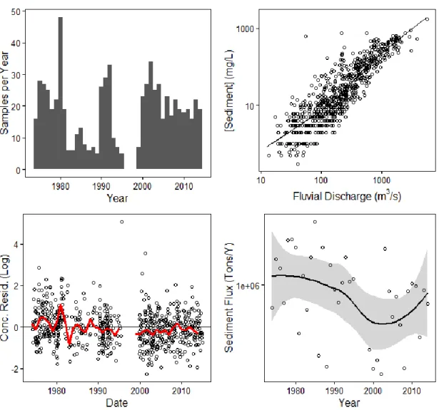
Sediment discharge is statistically modeled by taking the product of estimated sediment concentration and measured fluvial discharge. After additional corrective factors are applied, the predicted sediment flux is calculated as 𝑄𝑠(𝑡) = 𝐸 ∗ 𝑄(𝑡) ∗ 𝐶𝑠(𝑄(𝑡)) ∗ exp[𝑟(𝑦)] (Cohn 1995; Warrick et al. 2013). Qs(t) is the estimated daily discharge of sediment [mass/time]. Q(t) is the mean daily streamflow measured by stream gage [volume/time]. Cs(Q(t)) is the mean daily sediment concentration [mass/volume] predicted by fluvial discharge via regression (e.g. Fig. 2.1B). r(y) is the median of the log-residuals between measured and estimated Cs within the year sediment flux is being predicted [dimensionless] (Fig. 2.1C).
E
is a factor for correcting against bias introduced by log-transforming the data [dimensionless]. A non-parametric smearing coefficient (Duan 1983) was used for the corrective factor in this study, as opposed to theparametric alternative (Ferguson 1986), because the parametric factor can overestimate in studies with high sample variance (Helsel and Hirsch 2002).
34
being flexible with non-linear trends in the sediment rating curve, this methodology is attractive for other reasons. Smoothing with loess is readily accessible with the base statistics package for the R-programming language (R Core Team 2016). Also, since loess is still a form of linear regression, sediment rating curves based on loess inherit many of the previously described methods of rating curve correction and prediction that once were applied to simple linear fits. Loess smoothers are locally weighted regressions, and the span of the weighing window must be supplied to the model by the analyst. Smaller spans would decrease the root mean square error (RMSE) of the model, but can introduce bias by overfitting the data. In this study, it is assumed that predicted sediment concentration monotonically increases as discharge increases. Therefore, monotonicity must influence selection of span width (Helsel and Hirsch 2002). Aside from this case-specific requirement and (Cleveland 1979)’s recommendation of visualizing potential trends in residuals, there are relatively few guidelines for optimal span selection.
An automated search procedure was adopted to select an optimum span width using a consistent set of rules. A loess regression was computed for each span value from .05 to .95 by increments of .01, where span values are fractions of the domain. All models that failed to increase monotonically were rejected. For instances where monotonically increasing models did not exist at any span, suspended sediment concentration was assumed to be the geometric mean of the concentration measurements at all discharge rates. Of the remaining fitted models, the one minimizing the generalized cross validation statistic (GCV) was selected. GCV is an
35
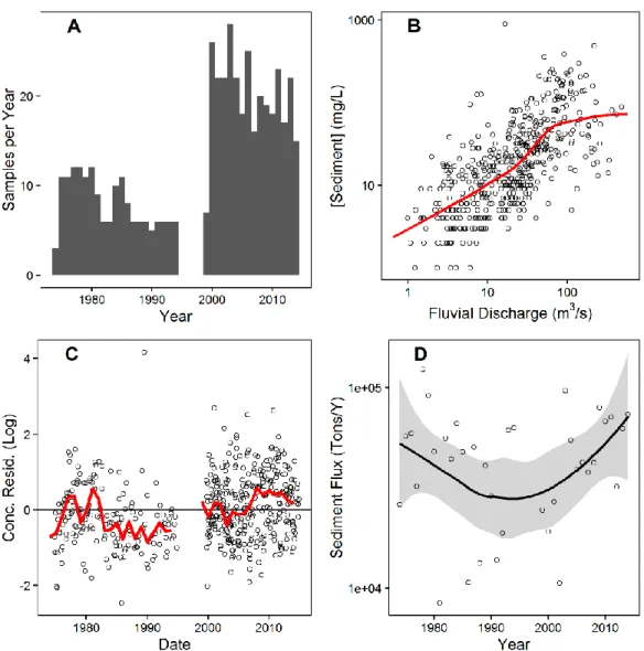
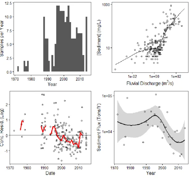
Figure 2.1- Example of Sediment Rating Curve Analysis:
An example site of the results from a sediment rating curve analysis to estimate suspended sediment flux at USGS gage #01673000 Pamunkey R. near Hanover, VA. A: Distribution of annual sediment collection. Sediment yield estimates were not made for years without samples.
B: Sediment concentration as a function of fluvial discharge. Best-fit loess curve is in red. C:
Residuals within each year, with median value in red. D: Annual cumulative sediment flux for each year sampled, with a .75 span loess smooth (95% confidence interval in grey) for
visualizing any trend. 2.2.4 Spatial Analysis:
36
downloaded from the NHDPlus website. For each watershed, the terminal catchment was determined by spatial overlay with the USGS gage’s coordinate (Latitude and Longitude
supplied by NWIS query). Unique identifiers (“COMID”s) for upstream catchments were found by recursive search using the TOCOMID and FROMCOMID attributes in the “PlusFlow” table. Catchment polygons were selected based on the acquired list of COMIDs and dissolved into a single polygon.
To characterize the flux of water into the basins being studied, precipitation data were acquired from the DAYMET (Thornton et al. 2014) surface weather database, comprised of 1 km square resolution gridded daily precipitation rates spanning from 1980 to present. The netcdf files were reformatted as rasters, and area-weighted average precipitation was measured each day for each watershed by extracting the raster values to overlying basin polygons. Snowfall was not explored in the precipitation analysis. Since the Piedmont is in the Southern United States, it is uncertain how much this will impact analysis.
Three different spatial datasets describing human behavior were extracted to the watershed polygons (Fig. 2.2). Illumination data was from annual averages of the DMSP Nighttime Lights time series (NCEI 2013) for years 1992 to 2014. Nighttime lights are 30 arc-second spatial resolution (approximately 1 km on a side), and its units are average visible band digital number (DN) values multiplied by the frequency of light detection. DN is a
37
map (30 meter resolution) (Fry et al., 2009; Fry et al., 2011; Homer et al., 2001; Vogelmann 2001).
Figure 2.2-Spatial Datasets of Human Behavior
The 2011 spatial datasets of human behavior extracted to the Piedmont polygon. A: Population
B: Night Lights C: Land cover type (Open water and transitional land types (e.g. barren, scrub/shrubland, etc.) were excluded from visualization)
38
2.3 Results
2.3.1: Sediment Flux Estimation Parameters:
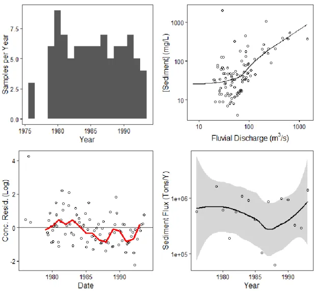
Variations in the sediment rating curve parameters are strongly controlled by the number of sediment samples collected at the gage site. Only sites with larger sample counts have shorter spans (Fig. 2.3C). This may be due to the points within loess’s weighting window having an averaging effect during the smoothing process, preventing more volatile vertical variations that are possible in sparsely populated datasets. At sufficiently narrow spans, local maxima and minima tend to form along the regression (Fig. 2.3A). This may explain why the monotonicity constraint appears to be a stronger determinant of span’s lower bound than the GCV statistic. Using data from the Chattahoochee at Whitesburg as an example, the span supplying a
monotonically increasing function is around two times as large as the span of minimum GCV (Fig. 2.3B).
39
40
Figure 2.3- Variation in Rating Curve Parameters
A: Sediment concentration vs. discharge at the Chattahoochee R. near Whitesburg with rating curves of variable span. B: GCV and monotonicity as a function of span at the Chattahoochee R. near Whitesburg. C: Optimal span vs. sample size. Triangular markers are the results of
41 2.3.2: Watershed Delineation Performance
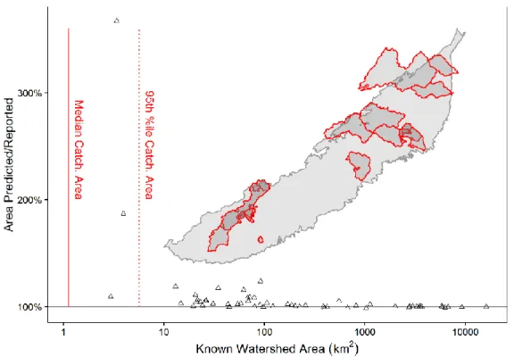
Known watershed areas were supplied for each gage station by the NWIS when data was queried. The area of the watersheds delineated using the NHDplus dataset was compared to these known values. Delineated watersheds are generally in good agreement with actual sizes, but appear to overestimate basin area by a small margin at most magnitudes (Fig. 2.4). The largest deviations occur as actual basin size approaches the resolution of the catchment polygons delineated by NHDplus. Catchment polygons tend to have a similar resolution to the raster datasets (Fig. 2.2). This means that the spatially extracted features of the smallest watersheds may reflect characteristics of neighboring watersheds as well as their own.
Fig. 2.4-Delineated Watersheds
42 2.3.3 Spatial Characteristics between Sites
Average within-watershed illumination follows what appears to be a saturation pattern with respect to population density (Fig. 2.5A). This may be related to limitations of the sensors on the satellite. This sigmoidal curve apparently separates the watersheds into urban vs. rural classifications, where light is indicative of urban infrastructure resulting from increased population density. Net changes in land cover from 2001 to 2011 support this intuition (Table 2.1). The horizontal line in Fig. 2.5A separates the watersheds into “high” vs. “low” illumination classifications (this classification will be described with more detail in the next section). Highly illuminated watersheds on average showed a larger net increase in developed land cover types and greater net losses in forested cover.
Table 2.1-Changes in Land Cover (2001-2011) [% of Watershed Area]:
Region Light Developed Forest Agriculture Transitional #sites
Georgia High 4.62% -1.41% 1.47% -4.68% 22
Georgia Low 0.39% -1.17% 4.50% -3.72% 7
Northern High 4.35% -1.42% 3.83% -6.76% 4
Northern Low 0.41% -0.41% 10.97% -10.97% 19
Net changes in land cover types within the Piedmont watersheds analyzed in the study. Changes were based on the NLCD 2001-2011 transition layer. Values are percentages of watershed area.
There are apparent sub-regions within this collected dataset, with roughly half of the watersheds clustered in the southwest Piedmont in Georgia, and the other half to the northeast predominantly in North Carolina and Virginia (Fig. 2.4). Despite an expected commonality in geomorphological features within the Piedmont, there are several notable points of
differentiation within the dataset that break down along this regional distinction.
43
in land cover are not uniform across regions either. Rates of deforestation are higher in
Georgia’s “low” light watersheds, while rates of increased agricultural coverage are higher in the northern “low” light watersheds (Table 2.1). There are also greater declines in transitional land types (Shrub/scrub, grassland/herbaceous, barren) across all northern watersheds.
The two regions also experience differences in hydrologically important characteristics. The watersheds selected for study have a broader distribution in the northern region, while the majority of Georgian watersheds tend to be relatively smaller in size (2.5E). There are
differences in rainfall as well, with the median annual rainfalls being roughly 15% higher than in northern watersheds.
44
Figure 2.5-Mean within-Site Characteristics:
A: Geometric mean of population vs. mean illumination (DN). GA sites in red. Error bars are range of values where yield was calculated. Blue .75 loess added for visualization. B:
Geometric mean of population vs. geometric mean of sediment yield, colored by mean illumination. Red loess curve for trend. C: Geometric mean of sediment yield vs. mean
illumination. A step function is in red, with geometric mean values and cut point annotated. The red ribbon is the geometric standard deviation. D: Boxplots of sediment yield vs. light group and region. Annotations are the number of sites. E,F,G: Boxplots of basin averages between
45 2.3.4 Sediment Yield Comparisons:
Despite the potential collinearity of rainfall, illumination, and watershed area, site mean sediment yields only appear to have a strong relationship with respect to illumination. Individual linear regressions of log(Yield) vs. illumination, log(area), and annual rainfall only saw
statistically significant relationships with respect to illumination (r2 = .5; p < .001). This relationship was used to develop the categorical variables of “high” vs. “low” light described earlier. The step-function of illumination vs. sediment yield where mean yield [tons/km2/year] equals 14.1 at low light (< 35.2) and 187.6 at high light (>35.2) (Fig. 2.5C) was based on this relationship. The cut point in illumination (35.2) was found by choosing a cut point which minimized the sum square error of a linear regression where log(Yield) is predicted by a categorical variable with values of “high” or “low”.