ІНФОРМАЦІЙНО
-
КОМУНІКАЦІЙНІ
ТЕХНОЛОГІЇ
ТА
МАТЕМАТИЧНЕ
МОДЕЛЮВАННЯ
UDC 621.311.61
S. S. BELIMENKO
1*, V. O. ISHCHENKO
2, V. O. GABRINETS
31*LLC «Teplotehnika», Yavornytskyi D. Ave., 102, Dnipro, Ukraine, 49000, tel./fax +38 (0562) 33 33 06, e-mail [email protected], ORCID 0000-0002-9935-4778
2Dep. «Heat Engineering», Dnipropetrovsk National University of Railway Transport named after Academician V. Lazaryan, Lazaryan St., 2, Dnipro, Ukraine, 49010, tel./fax +38 (056) 373 15 76, e-mail [email protected], ORCID 0000-0002-5948-9483 3Dep. «Heat Engineering», Dnipropetrovsk National University of Railway Transport named after Academician V. Lazaryan, Lazaryan St., 2, Dnipro, Ukraine, 49010, tel. +38 (056) 373 15 87, e-mail [email protected], ORCID 0000-0002-6115-7162
MODELING OF TEMPERATURE FIELDS IN A SOLID HEAT
ACCUMULLATORS
Purpose. Currently, one of the priorities of energy conservation is a cost savings for heating in commercial and residential buildings by the stored thermal energy during the night and its return in the daytime. Economic effect is achieved due to the difference in tariffs for the cost of electricity in the daytime and at night. One of the most com-mon types of devices that allow accumulating and giving the resulting heat are solid heat accumulators. The main purpose of the work: 1) software development for the calculation of the temperature field of a flat solid heat accu-mulator, working due to the heat energy accumulation in the volume of thermal storage material without phase tran-sition; 2) determination the temperature distribution in its volumes at convective heat transfer. Methodology. To achieve the study objectives a heat transfer theory and Laplace integral transform were used. On its base the prob-lems of determining the temperature fields in the channels of heat accumulators, having different cross-sectional shapes were solved. Findings. Authors have developed the method of calculation and obtained solutions for the determination of temperature fields in channels of the solid heat accumulator in conditions of convective heat trans-fer. Temperature fields over length and thickness of channels were investigated. Experimental studies on physical models and industrial equipment were conducted. Originality. For the first time the technique of calculating the temperature field in the channels of different cross-section for the solid heat accumulator in the charging and dis-charging modes was proposed. The calculation results are confirmed by experimental research. Practical value. The proposed technique is used in the design of solid heat accumulators of different power as well as full-scale produc-tion of them was organized.
Keywords: solid heat accumulator; thermal storage material
Introduction
Currently, one of the priority areas of energy-efficiency is to save costs on heating in industrial and residential buildings by the stored thermal en-ergy at night time and its return in the daytime. As a result, savings are achieved due to the difference in tariffs for cost of electricity in the daytime and at night one. Change to «Night» tariff allows pay-ing for electricity on an average three times
tem-perature field on the surface or in the volume of the object. Thermal storage devices are most widely used in the energy, engineering, transportation, chemical industry, agriculture. Consequently, re-search and development of methods for determining the operating modes and the weight and dimensional parameters of HA is an important task of energy con-servation, actual in the contemporary conditions of energy deficit.
Purpose
To date a large number of works about HA were published. The functioning of the HA in the process of heat storage can be realized by two main mechanisms: the first is due to changes of the physical parameters in the thermal storage solid (TSS); the second – through the use of the binding energy between atoms and molecules of sub-stances.
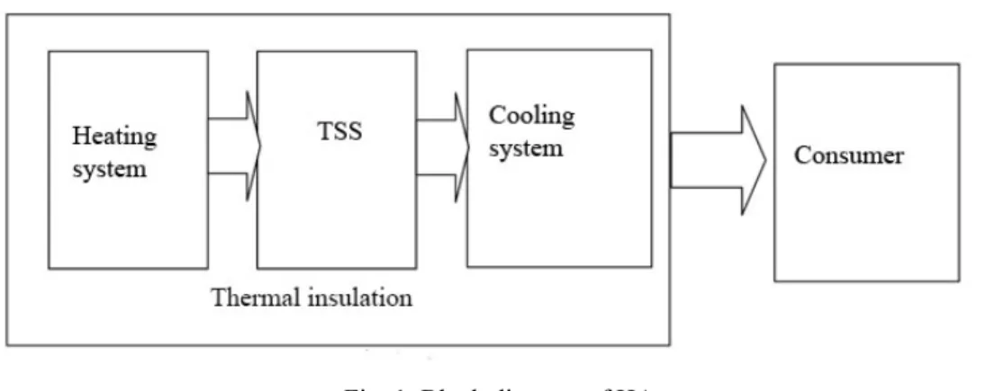
Capacitance-type batteries are the most com-mon and simple. Heat capacity of substance, heat-ing without its aggregative state change is used in them. Typical HA structural scheme is shown in Figure 1. It shows that HA always consists of insu-lated and thermal storage solid (TSS), heater, cool-ing systems, safety, regulation of heat supply and removal.
For the weight and dimension calculations one limits with mass determination [1]. In determining the HA modes, one considers the heat transfer pro-cesses using classical approaches of thermal fields analysis, as well as techniques based on mathe-matical modeling of heat transfer [7]. Mathemati-cal models of HA functioning are focused on the description of the HA thermal field [8-10] and cannot be directly applied for calculations of tem-perature field distribution, for example, when
con-vective heat transfers on the HA charge and dis-charge mode. In order to determine temperature stresses one can use [9]. However, proposed before calculation methods [10-14] do not reflect the pic-ture of heat transfer at active convective transfer occurring at HA charging / discharging.
The main objective of the work is to develop a method for calculating the temperature field TSS in the process of heat accumulation and removal at the design stage on the basis of mathematical mod-eling of the temperature field in condition of strong convective heat transfer.
Solid HA is a complex of multiple systems connected in a single structure constructively. Heating system is a mandatory element of the HA, in our case it is tubular heating elements (THEs). Heat generated by them is accumulated in the thermal storage solid of – HA charging is made. To use the stored heat, HA has a cooling system, in our case there are air channels. With the active cir-culation of the coolant – air, heat is removed from the TSS and supplied to the consumer. Heat-distribution system within the heating object space does not include in to HA complex.
The design concept of solid HA with convec-tive heat transfer is shown in Figure 2. HA consists of a jar 1 which can be fixed on any rigid support, the front jar is closed with battery cap 2, on the jar thermal insulation 3, 4 is fixed, in which TSS 5 is placed. On the front surface of TSS finger baffles 6 are mounted for the cooling air flow direction, which is fed to the bottom of TA through incoming louvers 7, then, passing through the HA channels, enters to the mixer 8 and go through the outlet lou-vers 9 falls within the scope of the object of heat supply.
Fig. 2. HA structural scheme
Methodology
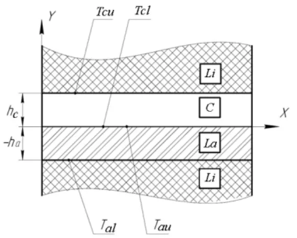
Design scheme for the analysis of the tempera-ture field in the HA can be shown in Fig. 3, where the following notation is introduced:
Li – heat insulation layer; C – channel; La – layer of ТSS, Tcu – the temperature of the upper boundary of the channel; Tcl – the temperature of the lower boundary of the channel Tau – the tem-perature of the upper boundary of ТSS; Tal – the temperature of the lower boundary of ТSS.
Fig. 3. Diagram of the temperature field analysis If we neglect the change of heat fluxes along the coordinate x, which is directed perpendicular to the plan of ТSS 5 (Fig. 2), the temperature field will depend on three independent variables, name-ly: spatial coordinates y and z, and time t. Using ratio t z V= 1, where V1 there is air movement velocity on the channel C, one can reduce constitu-tive equations to the form, where two independent
variables y и z will take place. Then we can write such heat transfer equations for the system shown in Fig. 3
2
1 1
1 p1 2 1 1 2
T T
C V
z y
∂ ∂
ρ ⋅ ⋅ ⋅ ⋅ = λ ⋅
∂ ∂ ; (1)
2
2 2
2 p2 1 2 2
T T
C V
z y
∂ ∂
ρ ⋅ ⋅ ⋅ = λ ⋅
∂ ∂ , (2)
where ρ, Cp, λ − thermal and physical character-istics of the material: density, heat capacity ratio and conductivity coefficient (subscripts 1 and 2 are used respectively for air and TSS); T − tempera-ture.
Each of the two equations will have two boundary conditions on the coordinate y and on one initial condition on the coordinatez.
The presence of the thermal insulation on the upper boundary of the channel, and the lower boundary of the TSS let neglect with heat flow out the heat accumulator boundaries, in other words one can record
1 0
T y ∂ =
∂ at y h= 1; (3)
2 0
T y ∂ =
∂ at y= −h2. (4) Two other boundary conditions can be
repre-sented as
1
1 21
T q y ∂ λ ⋅ =
∂ at y=0; (5)
(
)
2
2 12 1b 2t
T
T T
y ∂
−λ ⋅ = α ⋅ −
∂ at y=0, (6)
where q21 − heat flow coming into the channel from the heated ТSS; T1b – coolant temperature at the bottom surface of the channel; T2t − tempera-ture at the top surface of ТSS; α12– heat transfer coefficients between the cooling coolant and the top surface of the heated ТSS.
Initial conditions correspondingly for equations (1) and (2) will be
1 1( )
T = f y at z=0; (7)
2 2( )
where f y1( ), f y2( ) − temperature functional de-pendences from the coordinate y.
In the first approximation temperature func-tional dependences can be taken as constants. Then instead of (7) and (8) there will be
1 1n
T =T at z=0; (9)
2 2n
T =T at z=0. (10)
To solve equations (1) and (2) we use the La-place integral transformation [13, 14].
Using the theorem about the differentiation of the original, we obtain the operator analogs of equa-tions (1) and (2) in such form
2 1 1 1 2 1 1 L
L Tn
d T s
T
a a
dy − ⋅ = − ; (11)
2 2 2 2 2 2 2 L
L T n
d T s
T
a a
dy − ⋅ = − , (12)
where TL – temperature image T , including ap-propriate indexes; s – Laplace transformation var-iable;
(
)
1 1 2 1 p1 1
a = λ ⋅ρ ⋅C ⋅V ; a2= λ2
(
ρ ⋅2 Cp2⋅V1)
.Thus, using the Laplace integral transforma-tion, the transition from partial differential equa-tions (1) and (2) (in originals) to the differential equations in ordinary derivatives (in images), that are solved much easier.
Operator equations for the boundary conditions (3) – (6) will look like this
1L 0
dT
dy = at y h= 1; (13)
2L 0
dT
dy = at y= −h2; (14)
1 21
1
L
dT q
dy s
λ ⋅ = at y=0; (15)
1 2 2 2 12 L b t T T dT
dy s s
⎛ ⎞
−λ ⋅ = α ⋅⎜ − ⎟
⎝ ⎠ at y=0. (16)
Solutions of equations (11) and (12) have the form
1
1 11
1 sinh
L Tn s
T C y
s a ⎛ ⎞ = + ⋅ ⎜⎜ ⋅ ⎟⎟+ ⎝ ⎠ 12 1 cosh s C y a ⎛ ⎞ + ⋅ ⎜⎜ ⋅ ⎟⎟
⎝ ⎠; (17)
2
2 21
2 sinh
L Tn s
T C y
s a ⎛ ⎞ = + ⋅ ⎜⎜ ⋅ ⎟⎟+ ⎝ ⎠ 22 2 cosh s C y a ⎛ ⎞ + ⋅ ⎜⎜ ⋅ ⎟⎟
⎝ ⎠. (18)
For determining the integration constantsC11,
12
C , C21 and C22 it is necessary to differentiate the last two equations on coordinate y and substi-tute boundary conditions (13) – (16).
Substituting boundary conditions (13) and (15) into equation (17), as well as − (14) and (16) into equation (18), we obtain (after determining the integration constantsC11, C12, C21 and C22) such equations in the images for determining the tem-perature fields
(
1)
1 21 1 1 1 1 1 1 cosh 1 sinh L n s h y a q a T T
s s s s
h a ⎡ ⎤ ⋅ − ⎢ ⎥ ⋅ ⎣ ⎦ = − ⋅ ⋅
λ ⋅ ⎛ ⎞
⋅ ⎜ ⎟ ⎜ ⎟ ⎝ ⎠ ; (19)
(
)
12 2 1 2
2 2
2
b t L Tn a T T
T
s s
α ⋅ ⋅ −
= − ×
λ ⋅
(
2)
2 2 2 cosh 1 sinh s h y a s s h a ⎡ ⎤ ⋅ + ⎢ ⎥ ⎣ ⎦ × ⋅ ⎛ ⎞ ⋅ ⎜ ⎟ ⎜ ⎟ ⎝ ⎠ ; (20)
Taking into account an expression (16) and (20), one can write down such ratio at y=0
1 2
21 12 b t
T T
q
s s
⎛ ⎞
= −α ⋅⎜ − ⎟
⎝ ⎠.
(
)
12 1 1 2
1 1
1
b t L Tn a T T
T
s s
α ⋅ ⋅ −
= + ×
λ ⋅
(
1)
11 1
1
cosh s h y sinh s h
a a
s
⎡ ⎤ ⎛ ⎞
× ⋅ ⎢ ⋅ − ⎥ ⎜⎜ ⋅ ⎟⎟
⎣ ⎦ ⎝ ⎠; (21)
In order to go from the temperature image to the original, write the hyperbolic functions through exponential
(
)
cosh( )x = ex+e−x / 2,sinh( )x =
(
ex−e−x)
/ 2).After appropriate changes expression (21) can be presented as follow
(
)
12 1 1 2
1 1
1
b t L Tn a T T
T
s s
α ⋅ ⋅ −
= + ×
λ ⋅
(
)
0 1
exp 1k k d s s ∞ = × ⋅
∑
− ⋅ +(
)
0 1exp 2k k
d s
s
∞
=
+ ⋅
∑
− ⋅ , (22)where
[
1]
1 1
1k 2
d y h k
a = ⋅ + ⋅ ⋅ ;
(
)
1 1 12k 2 1
d y h k
a
= ⋅ ⎡− + ⋅ ⋅ + ⎤⎣ ⎦.
By analogy with the expression (22) one can convert the equation (20), namely
(
)
12 2 1 2
2 2
2
b t L Tn a T T
T
s s
α ⋅ ⋅ −
= − ×
λ ⋅
(
)
0 1
exp 3k k d s s ∞ = × ⋅
∑
− ⋅ +(
)
0 1exp 4k k
d s
s
∞
=
+ ⋅
∑
− ⋅ (23)where
[
2]
2 1
3k 2
d y h k
a = ⋅ − + ⋅ ⋅ ;
(
)
2 2 14k 2 1
d y h k
a
= ⋅ ⎡ + ⋅ ⋅ + ⎤⎣ ⎦.
Using the general formula of transition from the image to the original [2]
(
)
21 1 exp exp 4 C C s z s z ⎛ ⎞ ⋅ − ⋅ ↔ ⋅ ⎜− ⎟ ⋅
π⋅ ⎝ ⎠ (24)
and multiplication theory (Borel theorem) one can obtain from the expression (22) such original for temperature distribution in the solid plug along the y-axis
(
)
12 1 1 2
1 1
1
( , ) b t
n
a T T
T y z =T +α ⋅ ⋅ − ×
λ
[
E X y z1 ( , )1 E X y z1 2( , )]
× + (25)
where
2 1
0
1 1 ( , ) 2 exp
4 k
k
d z
E X y z
z
∞
=
⎡ ⎛ ⎞
= ⎢ ⋅ π⋅ ⎜− ⋅ ⎟−
⎢ ⎝ ⎠ ⎣
∑
1 1 2 k k d d erfc z ⎤ ⎛ ⎞ − ⋅ ⎜ ⎟⎥ ⋅ ⎝ ⎠⎦, 2 0 1 ( , ) 2k
z
E X y z ∞
= ⎡ = ⎢ ⋅ × π ⎣
∑
2 2 2 exp 2 4 2 k k k d d d erfc z z ⎤ ⎛ ⎞ ⎛ ⎞ × ⎜− ⋅ ⎟− ⋅ ⎜⎝ ⋅ ⎟⎠⎥⎥ ⎝ ⎠ ⎦Using the same technique as in the obtaining of expression (25), we find from (23) the original for temperature field distribution in the TSS
(
)
12 2 1 2
2 2
2
( , ) b t
n
a T T
T y z =T −α ⋅ ⋅ − ×
λ
[
E X y z2 1( , ) E X y z2 2( , )]
× + , (26)
where
2 1
0
3 2 ( , ) 2 exp
4 k
k
d z
E X y z
z
∞
=
⎡ ⎛ ⎞
= ⎢ ⋅ π⋅ ⎜− ⋅ ⎟−
2
0 2 ( , ) 2
k
z
E X y z ∞
=
⎡
= ⎢ ⋅ ×
π ⎣
∑
2
4 4
exp 4
4 2
k k
k
d d
d erfc
z z
⎤
⎛ ⎞ ⎛ ⎞
× ⎜− ⎟− ⋅ ⎜ ⎟⎥
⋅ ⎝ ⋅ ⎠⎥
⎝ ⎠ ⎦.
To determine the heat transfer coefficient α12
in equations (25) and (26) one can use expression in common case [15]
1 12
e
Nu b
⋅λ
α = (27)
where Nu – Nusselt criterion; be – equivalent size of the channel.
In general case, it is divided into three modes: turbulent
(
Re 10000>)
; transitional(
2300 Re 10000≤ ≤)
and laminar(
Re 2300<)
. In the case of turbulent regime one can use the following expression to determine the Nusselt cri-terion0,8 0,021 l Re
Nu= ⋅ε ⋅ ×,
0,25
0,43 Pr
Pr
PrWT
⎛ ⎞
× ⋅⎜ ⎟
⎝ ⎠ (28)
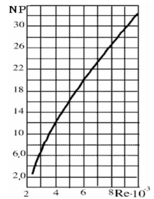
where εl – a correction factor that takes into ac-count impact of the ratio of the cooling cavity length L0 to its equivalent size be on the heat transfer coefficient; Re – Reynolds criterion; Pr – Prandtl number; PrWT – Prandtl number at a wall temperature of the cooling cavity. For transitional regime calculation is recommended to carry out by the graph, shown in Figure 4, at this the value
NPis determined by expression
(
)
0,250,43
Pr Pr PrWT
NP Nu= ⎡⎣ ⋅ ⎤⎦. (29)
The following relationship is the most accept-able for laminar regime
0,33 0,43 0,15 l Re Pr
Nu= ⋅ε ⋅ ⋅ ×,
0,25 0,1 Pr
Gr
PrWT
⎛ ⎞
× ⎜ ⎟
⎝ ⎠ (30)
where Gr – Grashof number.
To determine the criteria, one can use such ex-pressions
1 1
1 Re=V b⋅ ⋅ρe
η ;
1 1
1 Pr=Cp ⋅η
λ ;
3 2
1 2 1
Gr= g b⋅ ⋅ρe ⋅β ⋅ ∆T
η , (31)
where η1 – viscosity coefficient of a cooling me-dium; β – coefficient of volume expansion; ∆T – the temperature difference between the wall sur-face and the cooling liquid.
The correction factor decreases when increase the ratio of the cooling cavity length L0 to its equivalent size. When performing the ratio
0 e 50
L b > one can accept ε =l 1.
Fig. 4. The graph to determine the Nusselt criterion for the transitional regime
Equivalent size can be determined from the
formula be 4 Sg P ⋅
= ,
whereSg – square of effective cross-section; P – full (wetted) perimeter, regardless of what part of the perimeter is involved in heat transfer.
For heating liquid fluid one can take
(
)
0,25Pr PrWT ≈1.
taken as constant ones. In reality, they will depend on the coordinate zj. To take into account the last remark and achieve the required accuracy of calcu-lations, it should T1b and T2t to find on short seg-ments along z axle.
The initial values T1n and T2n are also should be constantly changed at each segment. Thus, the final values of the temperature field distribution on the previous segment will correspond to the initial values at the next segment along the axis z.
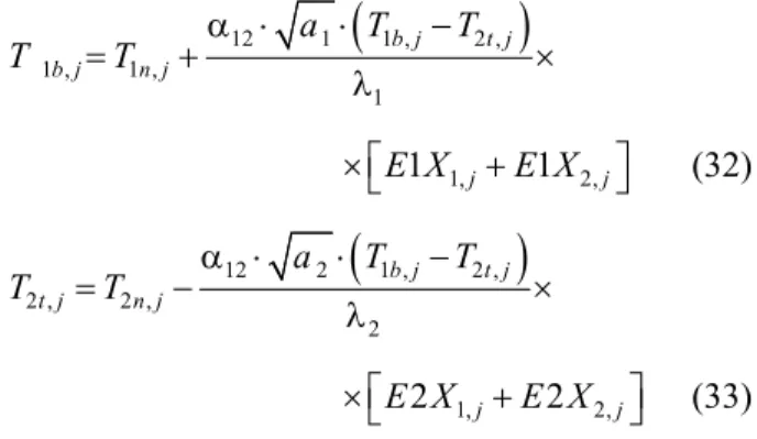
For determining the unknown boundary tempera-ture values from these equations, we obtain the following system of equations
(
)
12 1 1 , 2 ,
1 , 1 ,
1
b j t j b j n j
a T T
T =T +α ⋅ ⋅ − ×
λ
1, 2,
1 j 1 j
E X E X
⎡ ⎤
×⎣ + ⎦ (32)
(
)
12 2 1 , 2 ,
2 , 2 ,
2
b j t j t j n j
a T T
T =T −α ⋅ ⋅ − ×
λ
1, 2,
2 j 2 j
E X E X
⎡ ⎤
×⎣ + ⎦ (33)
In the last two equations index j characterizes the values of the corresponding ones on each seg-ment zj at zero value for the second coordinate (y=0).
For convenience, the solution of equations (32) – (33) are presented in a matrix form
1 , 0,0 0,1 0
2 , 1,0 1,1 1
b j
t j
T A A CV
T A A CV
⎡ ⎤ ⎡ ⎤ ⎡ ⎤
⋅ =
⎢ ⎥ ⎢ ⎥ ⎢ ⎥
⎣ ⎦
⎣ ⎦
⎣ ⎦ , (34)
where
12 1
0,0
1
1 a 1 j
A = −α ⋅ ⋅E X
λ ; 0,1 12 1
1
1 j
a
A =α ⋅ ⋅E X
λ ;
12 2
1,0
2
2 j
a
A =α ⋅ ⋅E X
λ ;
12 2
1,1
2
1 a 2 j
A = −α ⋅ ⋅E X
λ ;
1, 2,
1 j 1 j 1 j
E X =E X +E X ;
1, 2,
2 j 2 j 2 j
E X =E X +E X ;
0 1 ,n j
CV =T ;CV1=T2 ,n j.
To solve the above problem program block in the mathematical MathCAD package was devel-oped. Re-solving results are shown in Fig. 4, 5. In this case the initial values are following:
3 1 1,2kg/m
ρ = ,
1 0,0281 W /(m K)
λ = ⋅ , Ср1=1,03Kj/(kg K)⋅ ,
5 1 2,27 10 Pa s−
η = ⋅ ⋅ , 3
2 3200 kg/m
ρ = ,
2 1,93 W /(m K)
λ = ⋅ , Ср2 =0,57 Kj/(kg K)⋅ ,
1 0,3 m/s
V = ; h1=20 mm; h2 =60 mm;
2000 mmL= .
The indices correspond to the following desig-nations: 1-channel, 2-TSS. Designations corre-spond to Standards. One should take into consid-eration that the channel length L is determined by the number of baffles in HA.
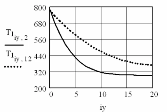
Length temperature behavior of TSS under specified conditions is shown in Fig. 5. The num-ber of partitions along the channel (iz) is 30, the number of partitions in channel depth and thick-ness of TSS (iy) is 20. The coordinate system corresponds to shown one in Figure 3.
Fig. 5. Length temperature curve of TSS at a fixed depth As can be seen from Fig. 5 the temperature at TSS, depth of 15mm increases from normal one – at the beginning of the channel and at a length of 2 m is already 570оС. In the mid-plane of TSS (iy=10), the temperature will be higher and 670оС.
de-pending on selection of calculation fixed point will be also insignificant and vary within 1-2оС.
Fig. 6. Temperature curve along the channel length, at a fixed depth
Temperature curve of TSS in depth at a fixed length and given conditions is shown in Fig. 7.
Fig. 7. Depth temperature curve of TSS at a fixed length As seen from the graph (Fig.7), depth tempera-ture behavior of TSS has exponential natempera-ture, in depth of TSS varies within 50оС.
Air temperature behavior in the channel in depth at a fixed channel length under given condi-tions is shown in Fig. 8.
As seen from the graph (Fig. 8), air temperature behavior in the channel in depth has a logarithmic character, by channel depth varies slightly within1-2оС.
After analyzing the above data, one can draw the following conclusion: temperature behavior of TSS in depth and length has exponential nature, it is more essential along the length than depth. Air temperature behavior in the length and depth of the channel varies insignificantly.
Fig. 8. Air temperature curve in the depth of the channel at a fixed length
Originality and practical value
Technical analysis shows that the proposed method of estimating the temperature field distri-bution of solid heat accumulator in different modes is effective, technically feasible and allows deter-mining the operation modes of the solid heat ac-cumulator at the specified weight and dimensional characteristics in the design stage of solid heat ac-cumulators.
Conclusions
The method of calculation for temperature fields of solid heat accumulators on charging / dis-charging modes was proposed.
LIST OF REFERENCE LINKS
1. Белименко, С. С. Разработкакритериевэффек
-тивности заряда и разряда твердотельного
теплового аккумулятора / С. С. Белименко,
В. А. Ищенко // Наукатапрогрестранспорту. – 2014. – № 5 (53). – С. 7−16. doi: 10.15802/-stp2014/29945.
2. Габринец, В. А. Оптимальнаяформатеплового аккумуляторасфазовымпереходомвтеплоак
-кумулирующем материале при вертикальном расположенииканалаподводаиотводатепла /
В. А. Габринец, И. В. Титаренко // Відновлю
-вальна енергетика 21 століття : матер. XIII
міжнар. конф. – Крим, 2012. – С. 285–289. 3. Габринец, В. А. Оптимизация грунтового
теплового аккумулятора / В. А. Габринец,
А. В. Трофименко, Л. В. Накашидзе // Відно
-влювальнаенергетикатаенергоефективністьу
21 столітті : матер. VII міжнар. наук.-практ.
4. Дан, П. Д. Тепловые трубы : [пер. с англ.] /
П. Д. Дан, Д. А. Рей. – Москва : Энергия, 1979. – 272 с.
5. Дружинин, П. В. Математическаямодель про
-цесса хранения теплоты в тепловом аккуму
-ляторе / П. В. Дружинин, А. А. Коричев,
И. А. Косенков // Технико-технолог. проблемы сервиса. − 2009. −№ 2. – С. 63−65.
6. Кузяев, И. М. Построениематематическихмо
-делейдля анализа температурныхнапряжений в рабочих элементах технических систем /
И. М. Кузяев, И. П. Казимиров, С. С. Белимен
-ко // Вопр. химииихим. технологии. – 2011. –
№ 6. – C. 211–217.
7. Левенберг, В. Д. Аккумулирование тепла /
В. Д. Левенберг, М. Р. Ткач, В. А. Гольстрем. –
Киев : Техника, 1991. – 315 с.
8. Лыков, А. В. Теория теплопроводности /
А. В. Лыков. – Москва : Высш. шк., 1967. – 600 с.
9. Лыков, А. В. Тепломассообмен / А. В. Лыков. –
Москва : Энергия, 1972. – 560 с.
10. Математическая модель процесса разрядки теплового аккумулятора фазового перехода /
П. В. Дружинин, А. А. Коричев, И. А. Косен
-ков, Е. Ю. Юрчик // Технико-технолог. про
-блемысервиса. – 2009. – № 4 (10). – С. 18–22. 11. Резницкий, Л. А. Тепловые аккумуляторы /
Л. А. Резницкий. – Москва : Энергоатомиздат, 1996. – 91 с.
12. McKechhie, J. The heat pipe: a list of pertient ref-erences / J. McKechhie // National Engineering Laboratory, East Kilbride. Applied Heat SR. BIB. –1972. – P. 2–12.
13. Feldman, К. Т. Applications of the heat pipe / K. T. Feldman, G. H. Whiting. / Mechanical Engi-neering. – 1968. – Vol. 90, № 11. – P. 48–53. 14. Behfard, M. Numerical investigation for finding
the appropriate design parameters of a fin-and-tube heat exchanger with delta-winglet vortex generators / M. Behfard, A. Sohankar // Heat and Mass Transfer. – 2016. – Vol. 52. – Iss. 1. – P. 21–37. doi: 10.1007/s00231-015-1705-1.
С
. C.
БЕЛІМЕНКО
1*,
В
.
О
.
ІЩЕНКО
2,
В
.
О
.
ГАБРІНЕЦЬ
31*ТОВ «Теплотехніка», пр. Д. Яворницького, 102, Дніпро, Україна, 49000, тел./факс +38 (0562) 33 33 06, ел. пошта [email protected], ORCID 0000-0002-9935-4778
2Каф. «Теплотехніка», Дніпропетровськийнаціональнийуніверситетзалізничноготранспортуіменіакадеміка В. Лазаряна, вул. Лазаряна, 2, Дніпро, Україна, 49010, тел./факс +38 (056) 373 15 76, ел. пошта [email protected], ORCID 0000-0002-5948-9483
3Каф. «Теплотехніка», Дніпропетровськийнаціональнийуніверситетзалізничноготранспортуіменіакадеміка В. Лазаряна, вул. Лазаряна, 2, Дніпро, Україна, 49010, тел. +38 (056) 373 15 87, ел. пошта [email protected], ORCID 0000-0002-6115-7162
МОДЕЛЮВАННЯ
ТЕМПЕРАТУРНИХ
ПОЛІВ
У
ТВЕРДОТІЛЬНИХ
ТЕПЛОВИХ
АКУМУЛЯТОРАХ
Мета. Наданийчасоднимізпріоритетнихнапрямківенергозбереженняє економіявитрат натеплопо
-стачаннявпромисловихтажитловихбудівляхзарахунокзбереженоїтепловоїенергіївнічнийчасівіддачі їїуденнігодини. Економічнийефектдосягаєтьсязарахунокрізницітарифівнавартістьелектричноїенергії вденнийінічнийчаси. Однимізнайбільшпоширенихтипівпристроїв, якідозволяютьакумулюватиівідда
-ватиотриманетепло, єтвердотільнітепловіакумулятори. Основнаметароботи: 1) розробкаматематичного забезпечення для розрахунку температурного поля плоского твердотільного теплового акумулятора, що працюєзарахунокнакопиченнятепловоїенергіївобсязітеплоакумулюючогоматеріалубезфазовогопере
-ходу; 2) визначеннярозподілутемпературивйогообсягахприконвективнійтеплопередачі. Методика. Для досягнення мети дослідження використані теорія теплопередачі та інтегральне перетворення Лапласа, на основіякоговирішенізадачі визначеннятемпературнихполівуканалахтепловихакумуляторів, щомають різні форми поперечного перерізу. Результати. Авторами розроблено методику розрахунку та отримано розв'язки длявизначеннятемпературнихполів уканалах твердотільногоакумуляторав умовахконвектив
-ноготеплообміну. Дослідженотемпературніполяподовжинійпотовщиніканалів. Проведеноексперимен
-тальнідослідження нафізичнихмоделяхіпромисловомуобладнанні. Наукова новизна. Впершезапропо
-нованометодикурозрахункутемпературного поля вканалах різногопоперечного перерізутвердотільного тепловогоакумулятораврежимахзарядкиірозрядки. Результатирозрахунківпідтверджуютьсяекспериме
-туваннітвердотільнихтепловихакумуляторів різної потужності; організовано серійневиробництвотепло
-вихакумуляторіврізноїпотужності.
Ключовіслова: твердотільнийтепловийакумулятор; твердийакумулюючийматеріал
С
. C.
БЕЛИМЕНКО
1*,
В
.
А
.
ИЩЕНКО
2,
В
.
А
.
ГАБРИНЕЦ
31*ООО «Теплотехника», пр. Д. Яворницкого, 102, Днипро, Украина, 49000, тел./факс +38 (0562) 33 33 06, эл. почта [email protected], ORCID 0000-0002-9935-4778
2Каф. «Теплотехника», Днепропетровскийнациональныйуниверситетжелезнодорожноготранспортаимени
академикаВ. Лазаряна, ул. Лазаряна, 2, Днипро, Украина, 49010, тел./факс +38 (056) 373 15 76, эл. почта [email protected], ORCID 0000-0002-5948-9483
3Каф. «Теплотехника», Днепропетровскийнациональныйуниверситетжелезнодорожноготранспортаимени
академикаВ. Лазаряна, ул. Лазаряна. 2, Днипро, Украина, 49010, тел. +38 (056) 373 15 87, эл. почта [email protected], ORCID 0000-0002-6115-7162
МОДЕЛИРОВАНИЕ
ТЕМПЕРАТУРНЫХ
ПОЛЕЙ
В
ТВЕРДОТЕЛЬНЫХ
ТЕПЛОВЫХ
АККУМУЛЯТОРАХ
Цель.Внастоящеевремяоднимизприоритетныхнаправленийэнергосбереженияявляетсяэкономияза
-трат натеплоснабжение в промышленных и жилых зданиях засчет запасенной в ночное времятепловой энергиииотдачиеевдневныечасы. Экономическийэффектдостигаетсязасчетразницытарифовнастои
-мостьэлектрическойэнергиивдневноеиночное время. Однимиз наиболеераспространенных типов уст
-ройств, которые позволяют аккумулироватьи отдаватьполученноетепло, являютсятвердотельные тепло
-выеаккумуляторы. Основнаяцельработы: 1) разработкаматематического обеспечениядлярасчета темпе
-ратурногополяплоскоготвердотельного тепловогоаккумулятора, работающегозасчетнакопления тепло
-вой энергии в объеме теплоаккумулирующего материала без фазового перехода; 2) определение распределения температуры в его объемах при конвективной теплопередаче. Методика. Для достижения целейисследованияиспользованытеориятеплопередачииинтегральноепреобразованиеЛапласа, наоснове которогорешены задачи определениятемпературныхполейв каналахтепловыхаккумуляторов, имеющих различныеформыпоперечногосечения. Результаты. Авторамиразработанаметодикарасчетаиполучены решениядляопределениятемпературныхполейвканалахтвердотельногоаккумуляторавусловияхконвек
-тивноготеплообмена. Исследованытемпературныеполяподлинеипотолщинеканалов.Проведеныэкспе
-риментальные исследования на физических моделях и промышленном оборудовании. Научная новизна.
Впервые предложена методика расчета температурного поля в каналах различного поперечного сечения твердотельноготепловогоаккумулятораврежимахзарядкииразрядки. Результатырасчетовподтверждают
-сяэкспериментальнымиисследованиями. Практическая значимость.Предложеннаяметодикаиспользует
-сяприпроектированиитвердотельныхтепловыхаккумуляторовразличноймощности; организованосерий
-ноепроизводствотепловыхаккумуляторовразличноймощности.
Ключевыеслова: твердотельныйтепловойаккумулятор; твердыйаккумулирующийматериал
REFERENCE
1. Belimenko S.S., Ishchenko V.A. Razrabotka kriteriyev effektivnosti zaryada i razryada tverdotelnogo teplo-vogo akkumulyatora [Development of criteria of charge and discharge efficiency of solid state of heat accumu-lator]. Nauka ta prohres transportu – Science and Transport Progress, 2014, no. 5 (53), pp. 7-16. doi: 10.15802/stp2014/29945.
2. Gabrinets V.A., Titarenko I.V. Optimalnaya forma teplovogo akkumulyatora s fazovym perekhodom v teploak-kumuliruyushchem materiale pri vertikalnom raspolozhenii kanala podvoda i otvoda tepla [Optimal shape of the heat accumulator with a phase transition in heat-accumulating material at a vertical position of supply and removal of heat]. Materialy XIII mizhnararodnoi konferentsii «Vidnovliuvalna enerhetyka 21 sto-littia» [Proc. of XIII Intern. Conf. «Renewable energy in the 21st century»]. Krym, 2012, pp. 285-289.
4. Dan P.D., Rey D.A. Teplovyye truby [Heat pipes]. Moscow, Energiya Publ., 1979. 272 p.
5. Druzhinin P.V., Korichev A.A., Kosenkov I.A. Matematicheskaya model protsessa khraneniya teploty v teplo-vom akkumulyatore [Mathematical model of the heat storage process in the heat accumulator]. Tekhniko-tekhnologicheskiye problemy servisa – Technical and Technological Service Problems, 2009, no. 2, pp. 63-65. 6. Kuzyaev I.M., Kazimirov I.P., Belimenko S.S. Postroyeniye matematicheskikh modeley dlya analiza tem-peraturnykh napryazheniy v rabochikh elementakh tekhnicheskikh sistem [Construction of mathematical mod-els for the analysis of thermal stress in the working elements of technical systems]. Voprosy khimii i khimicheskiye tekhnologii – Issues of Chemistry and Chemical Technologies, 2011, no. 6, pp. 211-217.
7. Levenberg V.D., Tkach M.R., Golstrem V.A. Akkumulirovaniye tepla [Heat storage]. Kiyev, Tekhnika Publ., 1991. 315 p.
8. Lykov A.V. Teoriya teploprovodnosti [Thermal conductivity theory]. Moscow, Vysshaya shkola Publ., 1967. 600 p.
9. Lykov A.V. Teplomassoobmen [Heat and mass transfer]. Moscow, Energiya Publ., 1972. 560 p.
10. Druzhinin P.V., Korichev A.A., Kosenkov I.A., Yurchik Ye.Yu. Matematicheskaya model protsessa razryadki teplovogo akkumulyatora fazovogo perekhoda [A mathematical model of the heat accumulator process for phase transition]. Tekhniko-tekhnologicheskiye problemy servisa – Technical and Technological Service Prob-lems, 2009, no. 4 (10), pp. 18-22.
11. Reznitskiy L.A. Teplovyye akkumulyatory [Heat accumulators]. Moscow, Energoatomizdat Publ., 1996. 91 p. 12. McKechhie J. The heat pipe: a list of pertient references. National Engineering Laboratory, East Kilbride.
Applied Heat SR. BIB. 2–12, 1972.
13. Feldman К.Т., Whiting G.H. Applications of the heat pipe . Mechanical Engineering, 1968, vol. 90, no. 11, pp. 48-53.
14. Behfard M., Sohankar A. Numerical investigation for finding the appropriate design parameters of a fin-and-tube heat exchanger with delta-winglet vortex generators. Heat and Mass Transfer, 2016, vol. 52, issue 1, pp. 21-37. doi: 10.1007/s00231-015-1705-1.
Prof. M. V. Gubinskiy, D. Sc. (Tech.) (Ukraine); Prof. V. G. Sychenko, D. Sc. (Tech.) (Ukraine) recommended this article to be published