warwick.ac.uk/lib-publications
Manuscript version: Author’s Accepted Manuscript
The version presented in WRAP is the author’s accepted manuscript and may differ from the
published version or Version of Record.
Persistent WRAP URL:
http://wrap.warwick.ac.uk/119658
How to cite:
Please refer to published version for the most recent bibliographic citation information.
If a published version is known of, the repository item page linked to above, will contain
details on accessing it.
Copyright and reuse:
The Warwick Research Archive Portal (WRAP) makes this work by researchers of the
University of Warwick available open access under the following conditions.
Copyright © and all moral rights to the version of the paper presented here belong to the
individual author(s) and/or other copyright owners. To the extent reasonable and
practicable the material made available in WRAP has been checked for eligibility before
being made available.
Copies of full items can be used for personal research or study, educational, or not-for-profit
purposes without prior permission or charge. Provided that the authors, title and full
bibliographic details are credited, a hyperlink and/or URL is given for the original metadata
page and the content is not changed in any way.
Publisher’s statement:
Please refer to the repository item page, publisher’s statement section, for further
information.
Xiaohan Ding1 Guiguang Ding1 Yuchen Guo1 Jungong Han2 Chenggang Yan3
Abstract
It is not easy to design and run Convolutional Neu-ral Networks (CNNs) due to: 1) finding the opti-mal number of filters (i.e., the width) at each layer is tricky, given an architecture; and 2) the com-putational intensity of CNNs impedes the deploy-ment on computationally limited devices. Oracle Pruning is designed to remove the unimportant filters from a well-trained CNN, which estimates the filters’ importance by ablating them in turn and evaluating the model, thus delivers high accu-racy but suffers from intolerable time complexity, and requires a given resulting width but cannot automatically find it. To address these problems, we propose Approximated Oracle Filter Pruning (AOFP), which keeps searching for the least im-portant filters in a binary search manner, makes pruning attempts by masking out filters randomly, accumulates the resulting errors, and finetunes the model via a multi-path framework. As AOFP enables simultaneous pruning on multiple layers, we can prune an existing very deep CNN with acceptable time cost, negligible accuracy drop, and no heuristic knowledge, or re-design a model which exerts higher accuracy and faster inference.
1. Introduction
Convolutional Neural Networks (CNNs) have become an important tool for many real-world applications and related research areas (Collobert & Weston,2008; LeCun et al.,
1990a;1995). Nowadays, designing a CNN usually means a tiring exploration in a vast design space, which usually
1
Beijing National Research Center for Information Science and Technology (BNRist); School of Software, Tsinghua Uni-versity, Beijing, China. Email: [email protected].
2
WMG Data Science, University of Warwick, Coventry, United
Kingdom3InstituteofInformationandControl, Hangzhou Dianzi
University, Hangzhou, China. Correspondence to: Yuchen
Guo <[email protected]>, Jungong Han <
Proceedings of the36th
International Conference on Machine Learning, Long Beach, California, PMLR 97, 2019. Copyright 2019 by the author(s).
includes the usage of non-linearities (ReLU, sigmoid or none), downsampling (max / average pooling or stride-2 convolution), shortcut connections (He et al.,2016), etc. With so many hyper-parameters in consideration, we still have to make a hard decision every time we use a convo-lutional layer: the number of filters, i.e., the width of the layer. Since an unnecessarily wide conv layer usually leads to meaningless parameters, heavy computational burdens, and overfitting, we wish to set a proper width for each layer, which is inherently tricky. In modern CNN architectures, some practical guidelines on the number of filters are fol-lowed. Taking VGG (Simonyan & Zisserman,2014) for example, when the feature maps are spatially downsampled by2×, the number of filters becomes2×, so that the com-putational burdens of each layer are kept roughly the same. Apparently, such guidelines leave much room to improve on the layer width for better accuracy and efficiency.
In this paper, destructive CNN width optimization refers to the process which takes a well-trained tidy CNN as input and produces an optimized one where some useless filters are removed. In this context, our method can be categorized into filter pruning, a.k.a. channel pruning (He et al.,2017) or network slimming (Liu et al.,2017), a family of CNN compression techniques, which features three strengths.1) Universality:filter pruning can handle any kinds of CNNs, making no assumptions on the application field, the network architecture or the deployment platform.2) Effectiveness: filter pruning effectively reduces the floating-point oper-ations (FLOPs) of the network, which serve as the main criterion of computational burdens. When a filter is pruned, its output channel and the corresponding input channels of the following layer are removed. That is, when several conv layers stacked together are pruned respectively, the total FLOPs are reduced quadratically. 3) Orthogonality: filter pruning simply produces a thinner network with no customized structure or extra operation, which is orthogonal to other model compression and acceleration techniques.
plays a vital role in the entire pipeline. By recognizing the unimportant filters, we diminish the accuracy drop, such that it becomes easier for the finetuning process to restore the ac-curacy. In this sense, the importance of filter can be defined by the network’s accuracy drop with the filter ablated. If we ablate a filter (i.e., mask out its outputs), test the model on an assessment dataset, and observe a severe accuracy drop, and then the filter can be defined as important.
The most straightforward and accurate algorithm to prune filters greedily by importance, which is referred to asOracle Pruning(Molchanov et al.,2016), can be implemented in a trial-and-error manner. For a specific layer, we ablate a filter, test the model on the assessment dataset, record the accuracy drop as the importance score, i.e., mean ac-curacy reduction (Abbasi-Asl & Yu,2017) or loss increase (Molchanov et al.,2016), then restore the filter and move on to the next filter. When all the filters have been tested, we prune the filter with the least importance score. However, when we start to prune the next filter, the relative importance of the remaining filters may have been changed (Sect.4.1), so they should be tested in the same manner again. In this way, we can slim a layer by always removing the filter with the least importance score until we are satisfied with the trade-off between accuracy and efficiency. However, for today’s CNNs where a conv layer can comprise hundreds of filters, the time complexity of Oracle Pruning is intolerable. In order to acquire the importance score of filters with rea-sonable time cost, some heuristic methods (Li et al.,2016;
Hu et al.,2016;Molchanov et al.,2016) have been proposed, which suffer from inferior quality of importance estimation, compared to Oracle Pruning (Fig.3). Of note is that “oracle” described here is only the most accurate greedypruning method. A better oracle would consider all combinations of pruned filters, but of course, this is extremely expensive.
In this paper, we propose Approximated Oracle Filter Prun-ing (AOFP), a multi-path trainPrun-ing-time filter prunPrun-ing frame-work (Fig. 1), where we keep searching for the next fil-ters to prune in a binary search manner and finetuning the model in the meantime, which features high quality of im-portance estimation, reasonable time complexity and no need for heuristic knowledge. The codes are available
at https://github.com/ShawnDing1994/AOFP.
Our contributions are summarized as follows.
• We improve unimportant filters selection by analyzing the outputs of the next layer only, rather than the final outputs. However, instead of solving a linear regres-sion problem layer-by-layer (Luo et al.,2017;2018), we ablate the filters randomly, then compute and accu-mulate the change in the next layer’s outputs, which is referred to as Damage Isolation. Doing so enables not only the faster importance estimation but also mutually independent pruning on all the layers simultaneously.
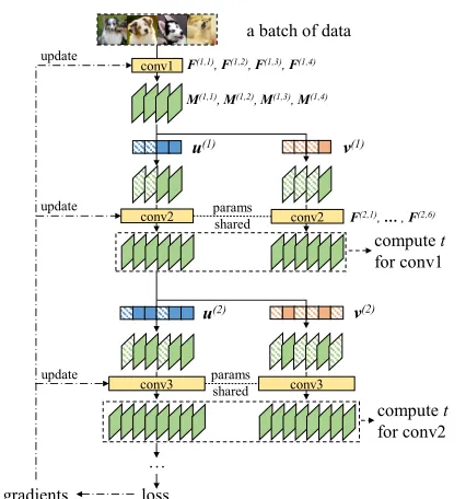
compute t for conv2 conv1
loss conv2
conv3
u(1) v(1)
u(2) v(2)
a batch of data
conv2
…
conv3
compute t for conv1
gradients update
F(1,1), F(1,2), F(1,3), F(1,4)
M(1,1), M(1,2), M(1,3), M(1,4)
F(2,1), … , F(2,6)
update
update params
[image:3.612.318.531.61.289.2]shared params shared
Figure 1.Overview of AOFP, where conv1 and conv2 in a
CNN are being pruned simultaneously for example. Filters
F(1,1),F(1,2),F(2,1),F(2,4)
have already been masked out, and the algorithm is trying to pick the next unimportant one out of
{F(1,3),F(1,4)}
and two out of{F(2,2),F(2,3),F(2,5),F(2,6)}
.
We have shown that the structural change of every layer in CNNs can be separately measured using only local information, which may inspire future researches. • Our experiments on CIFAR-10 and ImageNet have
shown the effectiveness of AOFP in significantly re-ducing the parameters and FLOPs of several very deep off-the-shelf CNNs including ResNet-152.
• We propose Destructive CNN Re-design, a CNN de-sign paradigm, which aims at optimizing the width of convolutional layers in order for higher accuracy and faster inference. E.g., the first two layers of VGG both have 64 filters, but we found out that 44 and 80 work better. This process can be used as a final refining step before a model is publicly released or deployed.
2. Related Work
Numerous researches (LeCun et al.,1990b;Hassibi & Stork,
1993;Castellano et al.,1997;Han et al.,2015b;Guo et al.,
2016) have proved it feasible to remove a large portion of pa-rameters from neural networks without significant accuracy drop. Furthermore, by removing filters instead of sporadic connections from CNNs, we transform the wide convolu-tional layers into narrower ones to reduce the FLOPs, mem-ory footprint and power consumption significantly.
E.g., a prior work prunes filters by the accuracy reduction with the filter ablated (Abbasi-Asl & Yu,2017); magnitude-based pruning (Li et al.,2016) considers the filters with larger magnitude more likely to be important; APoZ-based pruning (Hu et al.,2016) calculates the percentage of zeros in the activated feature maps; some researchers use Taylor-expansions (Molchanov et al.,2016). There are also some inspiring works which pick up filters by no importance score but by the channel contribution variance (Polyak & Wolf,
2015) or the Lasso regression (He et al.,2017).
A major drawback of the existing methods is the requirement for heuristic knowledge. 1)The filter importance metrics (Li et al.,2016;Molchanov et al.,2016;Hu et al.,2016) are heuristic, as it is not clear why the proposed metrics reflect the inherent importance of filters, and it is hard to judge if a heuristic method outperforms another.2)For iterative filter pruning methods, the granularity, i.e., the number of filters pruned at each step, is a key manually set hyper-parameter and a critical trade-off to be solved. The fewer filters are discarded once, the less damage is done to the model, which means the less finetuning time is required for the network to restore the accuracy; but more steps are needed to reach a satisfactory compression rate. 3)It is difficult to decide when to stop pruning, i.e., the resulting width of each layer. Many works (Li et al.,2016;Hu et al.,2016;He et al.,2017) have shown that some layers can be pruned by a large ratio without accuracy drop, but some layers are sensitive, which makes it hard to set layer-wise termination conditions.
Apart from pruning by importance, some other methods train the model under certain constraints (e.g., group Lasso (Roth & Fischer,2008)) in order to zero out some filters ( Al-varez & Salzmann,2016;Wen et al.,2016;Ding et al.,2018) or make them identical for removal (Ding et al.,2019).
Moreover, some other CNN compression and acceleration techniques have also been intensively studied, including ten-sor low rank expansion (Jaderberg et al.,2014), parameter quantization (Han et al.,2015a), knowledge distillation ( Hin-ton et al.,2015), DCT-based fast convolution (Wang et al.,
2016), feature map compacting (Wang et al.,2017b), etc. Of note is that AOFP is complementary to these methods.
3. Approximated Oracle Filter Pruning
3.1. Formulation
Letibe the layer index,M(i)∈
Rhi×wi×cibe anh
i×wi feature map withcichannels andM(i,j)=M
(i)
:,:,jbe thej -th channel. The parameters of conv layeriwith kernel size
ri×sireside in the kernel tensorK(i)∈Rri×si×ci−1×ci
and the bias termb(i)∈
Rci, so we useP(i)= (K(i),b(i))
to denote the parameters of layeri. In this paper, filterj
at layerirefers to the tuple comprising the trained param-eters related to the output channelj of layer i,F(i,j) =
(K:(,i:),:,j, b(ji)), and we denote the set of all such filters at layeribyFi. This layer takesM(i−1)∈Rhi−1×wi−1×ci−1
as input and outputsM(i). Let∗be the 2-D convolution operator, an arbitrary output channeljis
M(i,j)=σ(i)((
ci−1 X
k=1
M(i−1,k)∗K:(,i:),k,j) +b(ji)), (1)
whereK:(,i:),k,jis thek-th input channel of thej-th filter, i.e., a 2-D convolution kernel, functionσ(i)denotes the possible following operations such as non-linearities. For simplicity, we rewrite this transformation as a functionζ(i),
M(i)=ζ(i)(M(i−1),Fi). (2)
Importance-based filter pruning methods define the impor-tance of filters in terms of some measures, score the filters by some means, then prune the unimportant parts and re-construct the network using the remaining parameters. Let
T be the filter importance score value,δbe the threshold andIibe the filter index set of layeri(e.g., if conv5 has four filters, thenI5 ={1,2,3,4}), the remaining set, i.e.,
the index set of the filters which survive the pruning, is
Ri={j∈ Ii|T(F(i,j))> δ}. We prune the other filters
by reconstructing the network using the remaining parame-ters sliced from the original kernel and bias term. That is,
P(i)←(K:(,i:),:,R i,b
(i)
Ri). (3)
If the conv layer is followed by a batch normalization (Ioffe & Szegedy,2015) layer, its parameters should be handled in the same way as the bias termb. The input channels of the following layer corresponding to the pruned filters should also be discarded,
P(i+1)←(K:(,i:+1),R i,:,b
(i+1)).
(4)
3.2. Rethinking Oracle Pruning
In this subsection, we focus on the situation where we prune
qfilters from a layer which originally hascfilters. Oracle Pruning assesses a filter’s importance by looking at the model’s accuracy drop when the filter is ablated. Formally, letF be the original filter set of the CNN,L(x, y,F)be the accuracy-related loss value (e.g., cross-entropy loss for classification tasks) generated with the given filter set,X
andY be the examples and labels of the assessment dataset, which is a subset of the training dataset, thescoring process
aims to obtain the importance score for each filterF by
T(F) = X
(x,y)∈(X,Y)
(L(x, y,F −F)−L(x, y,F)), (5)
removed or equivalently masked out. In this way, we can slim a layer by always removing the filter with the least
T value and re-scoring the remaining filters for q times. Compared to the heuristic approaches, whereTis computed in other ways, an obvious strength of Oracle Pruning is the accuracy, while its weakness is the high time complexity. Specifically, using an assessment dataset ofγexamples, the time complexity of Oracle Pruning isO(cqγ), because we need to ablate every remaining filter in turn (O(c)) then test on the assessment dataset (O(γ)) to pick up a single filter to prune, and this scoring process is conducted forqtimes.
A straightforward way to alleviate the computational bur-dens is to prune several filters once at a time, trading accu-racy for efficiency. However, as all the filters at a conv layer compose a highly non-linear system (Mozer & Smolensky,
1989), removing a filter can affect the relative importance of other filters, inevitably resulting in poor accuracy (Fig.
3). We refer to the number of filters pruned at a time as the
granularityg. Except for lower accuracy, another downside of granular pruning is that we introduce an extra hyper-parameterg, which may require heuristic knowledge and human efforts to tune. For example, we can estimate the redundancy of a layer by pruning some filters and observing the accuracy drop in advance, such that we setgto a larger value to reduce the time cost if the layer seems to be highly redundant, or adopt a smallergto prune more carefully.
3.3. Damage Isolation
The essence of Oracle Pruning is to observe the conse-quences of the temporary removal of filters, i.e., to observe the feedback of many pruning attempts, which is generated by computing the final loss value. In this way, even when we are trying to prune a low-level layer, we still need to feed the input data through the entire network to obtain the feedback. Even worse, using such a feedback loop, we can only deal with one layer at a time, because as we ablate the filters in a specific layer, the subsequent information flow of the network is changed, such that the scoring processes of the higher-level layers are affected. Therefore, we seek to shorten the feedback loop for faster inference and mutually independent parallel filter scoring on every layer.
Our proposed approach is based on an intuition that a CNN can be viewed as a state machine, where the feature maps (states) are transformed by the operations performed by conv layers (Eq. 2). So essentially, the change in the filters at layeri, i.e., the change inM(i), is isolated by the
subse-quent layeri+ 1, because layeri+ 2and the higher-level layers cannot see the change inM(i). Taking the extreme
case for example, if we prune some filters at layeri, but observe no difference inM(i+1), we can claim that the pruning does no damage to the model because the input states to the remaining part of the network are not changed.
Inspired by this, we propose to calculate the approximated importance scoreT0based on the output of the next layer,
T0(F) = 1
|X|
X
x∈X
t(F, x), (6)
whereF is a filter at layeri,tis theisolated damage sample
which reflects how much the output of layeri+ 1on input examplexis deviated by the pruning attempt onF,
t(F, x) = ||M
(i+1)(x)−ζ(i+1)(M(i) F (x),F
(i+1))||2 2
||M(i+1)(x)||2 2
.
(7) HereMF(i)(x)is the output of layeriderived withoutF,
MF(i)(x) =ζ(i)(M(i−1)(x),Fi−F). (8)
Except for Euclidean distance, other distance functions may work as well, which are beyond the scope of this paper.
3.4. Multi-path Training-time Pruning Framework
It is common to finetune the whole model after each time of pruning (Li et al.,2016; Molchanov et al.,2016; Hu et al.,2016;Abbasi-Asl & Yu,2017), i.e., the scoring and finetuning processes are serial. To reduce the time cost, we propose a multi-path training-time pruning framework (Fig.
1) to parallelize the scoring and finetuning.
Specifically, when we prune a certain conv layeri, the com-putation flow after it is split into two paths, which are re-ferred to as the base path and the scoring path, respectively. E.g., Fig. 1shows two scoring paths which each contain only one conv layer (conv2, conv3) as we are pruning conv1 and conv2 simultaneously. The base path forwards the out-puts of layerithrough abase masku(i)∈
Rciinitialized as
1. Thej-th channel of the output of the next layer becomes
M(i+1,j)=σ(i+1)((
ci X
k=1
uk(i)M(i,k)∗K:(,i:+1),k,j) +b(ji+1)).
(9) It is obvious that settingu(ki)= 0is equivalent to removing thek-th filter at layeri. At the endpoint of the base path, the original loss value is calculated, the gradients are derived and the model parameters are updated. Meanwhile, the scoring path goes through ascoring maskv(i)∈
Rci, the
maskedM(i)is fed into layeri+1, then the isolated damage sampletis computed and stored in memory.
and more samples collected, we become more and more confident to tell which filters are the least important. When enough samples have been collected, we approximateT0for each filterjin the layer by
ˆ
T(F(i,j)) =mean(T(i,j)), (10)
whereT(i,j)is a set which records all thetvalues collected
with filterjablated.
With all the filters scored, we pick upgfilters with the lowest
ˆ
T value, fix the corresponding bits inu(i)andv(i)to zero, such that the filters are masked out permanently. Of note is that changing some bits inu(i)affects the back-propagation through the base path, thus the network’s accuracy will be restored by finetuning. In the meantime as finetuning, we choose the nextgfilters to prune through the scoring path. We refer to the process of choosing one or more filters to prune (in the meantime as recovering the damage caused by the last pruning) as a move. When some termination conditions have been met, we remove the filters according to the base mask by Eq.3,4withRi={j|u(ji)= 1}, such that the layer is slimmed with no further accuracy drop.
Such a multi-path framework enables parallel scoring and pruning on multiple layers, i.e., we can prune layeri ac-cording to the outputs of layeri+ 1and prune layeri+ 1
according to layeri+ 2simultaneously. Scoring a low-level conv layer does not affect the higher-level ones because ev-ery scoring process compares the outputs of the scoring path with the base path unaffected by the pruning attempts (i.e., the changes of the scoring masks) on the previous layers.
Note that though we randomly mask out channels in a dropout-like (Srivastava et al.,2014;Molchanov et al.,2017) manner, we do not rescale the remaining parts for compen-sation as we do when using dropout for regularization.
3.5. Binary Filter Search
In this subsection, we discuss and solve three problems of the proposed framework. 1) On a specific layer, the finetuning process makes the parallel scoring inaccurate. Whengfilters have been masked out permanently, i.e., the corresponding bits in the two masks have been fixed to zero, the network needs a period to recover, during which the filter importance assessment is not accurate. Namely, since the remaining filters vary during the finetuning period after the last pruning, thetvalues obtained in this period do not accurately reflect the actual importance of the filters which are being scored.2)The optimal value of the granularityg
is hard to resolve. 3)It is heuristic to decide when to stop pruning, as we do not know the optimal resulting width.
Inspired by the idea ofincremental refinement, we propose to search for the least important filters in a binary search manner. Concretely, at the beginning of each move, all the
Algorithm 1Approximated Oracle Filter Pruning
1: Input: the target layeriof the original CNN, refine-ment thresholdθ, search costφ
2: Base masku←1
3: whileTruedo
4: Search spaceA ← {j|uj = 1}
5: repeat
6: Loss record setT(i,j)← {},∀j∈ A
7: repeat
8: Randomly choose|A|/2elements out ofAas the ablated filter index setH
9: Initializev←u, letvj ←0,∀j∈ H
10: Generate and forward a batch of input data, com-pute thetvalue as Eq.7, record it for the ablated filters byT(i,j)← T(i,j)∪ {t},∀j∈ H
11: Back-prop gradients, update parameters
12: untilφbatches have been forwarded
13: ComputeTˆfor each filterj∈ Aas Eq.10
14: Pick up|A|/2filters with the smallestTˆvalue as the picked setB
15: Max damagep=max({Tˆ(F(i,j))| ∀j∈ B})
16: LetA ← B
17: untilp < θor|B|= 1
18: if p < θ ,then
19: Letuj ←0,∀j∈ B // prune the picked filters
20: else
21: break //p≥θand|B|= 1, stop refining
22: end if
23: end while
24: Prune layeriby Eq.3,4withRi ={j|uj= 1}
25: Return
remaining filters compose the search spaceA. We first score every filter inAand pick up|A|/2filters as the picked set B which are most likely to be unimportant. Though the network has not become stable (if this is not the first move), the assessment is not accurate indeed, but accurate enough for such a coarse-grained search. WhenBis obtained, the network finetuned through the base path has become more stable, so we abandon the collected samples and start a more fine-grained search by lettingA ← B, searching for the less important half of the picked set (i.e., a quarter of the last search space). As we use imprecise samples to do coarse searches and high-quality samples to search accurately, the samples collected in the meantime as finetuning are fully utilized, and the accuracy of importance scoring is guaran-teed. We refer to the number of collectedtsamples needed to complete one step of binary search as thesearch costφ.
Start
End Forward φ batches, select half of the filters
as the picked set
Continue refining?
Mask them out by setting the base mask, exclude them from the search space Good
enough? Use the picked set as
the new search space
Initialize the search space as all the filters
Prune according to the base mask
Yes No
Yes
[image:7.612.59.279.61.168.2]No
Figure 2.Flow chart of AOFP on a single layer.
manually set controlling conditions. Essentially, at each step of binary search, the picked set can be regarded as the least important|B|filters. If we finish the current move by pruning them,|B|serves exactly as the granularityg. So in the context of binary search, the problem of decidinggand the termination conditions can be simply solved as follows:
• If the current picked setBis good enough, finish the current move withg=|B|(i.e., permanently mask out the filters inBand start a new move); otherwise, see if it is possible to continue refining (|B|>1or|B|= 1). • If|B| >1, we continue refining by lettingA ← B; otherwise, it suggests that the single least important filter is still too important, so we stop pruning the layer.
We introduce a global hyper-parameter, the refinement thresholdθ, which is used to compare with the maxTˆvalue (Eq.10) of the filters inBto judge if the picked set is good (unimportant) enough. We sayBis good enough if
max({Tˆ(F(i,j))| ∀j∈ B})< θ . (11)
Intuitively,θindicates the upper limit of the damage we can endure for a single step of pruning. E.g., withθ = 0.02, we consider it acceptable to prune one or more filters with 2% isolated damage. With a largerθ, we tend to prune with larger granularity, and vice versa.
In this way, another design concern is settled naturally, that is, how many filters to randomly ablate for a batch of input data. We randomly ablate|A|/2filters out of the search spaceAat a time, and the reason is simple: according to our discussions above, the collectedtvalues should reflect the expected damage if we prune the current picked set, i.e., thetvalues should be derived with|B|filters ablated, and|B|=|A|/2. The AOFP algorithm on a single layer is outlined in Fig. 2and formally described in Alg. 1. In practice, we apply AOFP on every layer simultaneously.
4. Experiments
4.1. Comparison of Filter Pruning Metrics
In this subsection, we present a comparison of Oracle Prun-ing, AOFP and other heuristic methods using AlexNet (Krizhevsky et al.,2012) on ImageNet (Deng et al.,2009).
0 10 20 30 40 50 60 number of pruned filters
0.0 0.1 0.2 0.3 0.4 0.5
Top-1 accuracy
Oracle Pruning Oracle Pruning 10 × AOFP Degraded Oracle Magnitude Taylor APoZ Index
Figure 3.Comparison of filter pruning metrics on AlexNet.
We use the simplified version of AlexNet (GoogLe,2017a), which is composed of five stacked conv layers and three fully-connected layers with no LRU or cross-GPU connec-tions. For faster convergence, batch normalization (Ioffe & Szegedy,2015) is applied on every conv layer. We compare these metrics by pruning filters one by one from the first layer without finetuning. Fig.3shows the Top-1 accuracy on the validation set with varying number of pruned filters. For Oracle Pruning, APoZ-based and Taylor-expansion-based, we use randomly sampled 10,000 training examples as the assessment dataset. For AOFP, we set the search cost
φsuch that the total number of examples consumed equals that of Oracle Pruning. As we are pruning only one layer, we apply Binary Filter Search to collect the final loss value instead of the isolated damage. For Oracle Pruning10×, we use 100,000 examples to score a filter. For Degraded Oracle, no re-scoring processes are conducted, i.e., the im-portance scores collected at the very beginning are used to guide the pruning till the end. For the curve labeled as Index, we prune filters from the first one to the 64th, which is essentially equivalent to random guess.
Our observations are as follows.1)By comparing Degraded Oracle and Oracle Pruning, we conclude that re-computing importance scores after each step of Oracle Pruning is es-sential, as a CNN is a highly non-linear system, and the removal of a filter can affect the relative importance of other filters. This discovery is consistent with the observations of prior works (Mozer & Smolensky,1989;Sharma et al.,
2017) that neural networks do not distribute the learning representation equitably across neurons.2)AOFP is almost as good as Oracle Pruning. 3) The extra costs of Oracle Pruning10×bring marginal accuracy improvement.
4.2. AOFP for Automatic CNN Compression
[image:7.612.323.532.64.142.2]Table 1.Pruned VGG on CIFAR-10. The resulting models with different FLOPs are labeled from A1 to A5.
Result Top-1 FLOPs FLOPs↓%
base 93.38 313M
-AOFP-A1 93.81 215M 31.32
(Li et al.,2016) 93.40 206M 34.20
AOFP-A2 94.03 186M 40.51
(Liu et al.,2017) 93.80 - 51.00
(Huang et al.,2018) 91.67 - 55.20
AOFP-A3 93.84 124M 60.17
(Xu et al.,2018) 93.29 120M 61.46
AOFP-A4 93.47 108M 65.27
(Zhou et al.,2018) 92.33 - 74.81
AOFP-A5 93.28 77M 75.27
in the same manner as (He et al.,2016). Of note is that we perform AOFP on every target layer simultaneously. Con-cretely, for a specific layer, when the returning condition in Alg.1is satisfied, the AOFP process is restarted, i.e., we finish the current move without changing the base mask and start the next move. After each move on any conv layer, we calculate the reduced global FLOPs based on the model architecture and the current values of all the base masks, and stop pruning when the reduced FLOPs reach a target level (e.g., above 60% for the model labeled as AOFP-A3 in Table.1). Then we reconstruct a narrower network fol-lowing Eq.3,4for every layer, finetune the model, and test it on the validation dataset using a single central crop.
On CIFAR-10, we use VGG-16 for a quick sanity check. The base model is trained from scratch for 600 epochs to ensure the convergence, with the standard data augmenta-tion, i.e., padding to40×40, random cropping and flipping. We use a batch size of 64 and a learning rate initialized to
5×10⁻²then decayed by 0.1 every 200 epochs. We perform
AOFP on all of the 13 layers with search costφ= 20,000,
θ = 0.01and a constant learning rate of1×10−3. On
ImageNet, we first prune all the conv layers of AlexNet with
φ= 4,000,θ= 0.02and a learning rate of1×10−3. For
ResNets, since there are more layers being simultaneously pruned, we increase the search cost toφ= 8,000for better filter scoring and damage recovery. These hyper-parameters are casually set without careful tuning. Of note is that, on ResNets, due to the constraints of the shortcut connections, only the internal layers (i.e., the first and second layers in each block which are not directly added to the identity map-ping) are pruned, as a common practice (Luo et al.,2017;
Luo & Wu,2018;Wang et al.,2017a).
As it turns out (Table.1,2), these networks can be pruned significantly even with an increase in accuracy due to the optimized network structure, which is consistent with the observations in other works (Liu et al.,2017;Li et al.,2016). And if we wish to trade accuracy for efficiency, AOFP can reduce the computational burdens by a large margin,
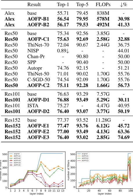
demon-Table 2.Pruning on ImageNet. The competitors include ThiNet
(Luo et al.,2017), NISP (Yu et al.,2018), Channel Pruning (He
et al.,2017), SPP (Wang et al.,2017a), Autopruner (Luo & Wu,
2018), ISTA-based (Ye et al.,2018), C-SGD (Ding et al.,2019).
Result Top-1 Top-5 FLOPs ↓%
Alex base 55.71 79.45 838M
-Alex AOFP-B1 56.54 79.95 578M 30.98
Alex AOFP-B2 56.17 79.53 492M 41.33
Res50 base 75.34 92.56 3.85G
-Res50 AOFP-C1 75.63 92.69 2.58G 32.88
Res50 ThiNet-70 72.04 90.67 2.44G 36.75
Res50 NISP 0.89↓ - - 44.01
Res50 Chan-Pr - 90.80 - 50.00
Res50 SPP - 90.40 - 50.00
Res50 Autopr 74.76 92.15 - 51.21
Res50 ThiNet-50 71.01 90.02 1.70G 55.76
Res50 C-SGD-50 74.54 92.09 1.70G 55.76
Res50 AOFP-C2 75.11 92.28 1.66G 56.73
Res101 base 76.63 93.29 7.57G
-Res101 AOFP-D1 76.88 93.49 5.29G 30.11
Res101 ISTA 75.27 - 4.47G 40.95
Res101 AOFP-D2 76.40 93.07 3.77G 50.19
Res152 base 77.37 93.52 11.28G
-Res152 AOFP-E1 77.47 93.76 6.12G 45.72
Res152 AOFP-E2 77.00 93.49 4.13G 63.36
Res152 AOFP-E3 76.40 93.02 2.85G 74.69
1 2 3 4 5 6 7 8 9 10 11 12 13 layer index
0 100 200 300 400 500
number of filters
original AOFP-A1 AOFP-A2 AOFP-A3 AOFP-A4 AOFP-A5
1 20 40 60 80 100 layer index
0 100 200 300 400 500
number of filters
[image:8.612.309.538.124.462.2]original AOFP-E1 AOFP-E2 AOFP-E3
Figure 4.Layer width of pruned models. Left: VGG on CIFAR-10.
Right: ResNet-152 on ImageNet (only the pruned layers).
strating not only higher pruning ratios but also less accuracy drop than other methods. Moreover, the increased network depth does not hinder the application of AOFP, because we simultaneously prune every layer in a mutually interdepen-dent manner, and do not suffer from the notorious problem of error propagation and amplification in filter importance estimation (Yu et al.,2018), thanks to Damage Isolation.
Of note is that AOFP automatically detects the easy-to-prune layers without heuristic knowledge or manually set control conditions, which is a significant strength compared to other approaches where we have to empirically decide the width of every layer in advance (Li et al.,2016;Luo et al.,
[image:8.612.309.538.125.466.2]Table 3.AOFP pruned v.s. uniformly slimmed VGG. All the mod-els are tested on an Nvidia GTX 1080Ti GPU or E5-2680 CPU with batch size 64, measured in examples/sec.
Top-1 FLOPs CPU GPU Speedup
VGG base 93.38 313M 343 6336
-AOFP-A3 93.84 124M 683 13903 2.19×
Uniform 92.88 126M 560 10224 1.61×
pruning ratios. Similarly, AOFP converts the original tidy ResNet-152 to a more efficient one without human inter-vention. One concern about the irregularly shaped models is that the varying width of layers may cause GPU mem-ory bottlenecks, so it may not result in real acceleration, though the FLOPs are reduced. However, our pruned VGG outperforms a uniformly slimmed counterpart in both ac-curacy and speed (Table. 3). Concretely, we construct a VGG model where every layer is 69% of its original width, such that the FLOPs becomes 126M, which is comparable to our pruned model labeled as AOFP-A3. We train it from scratch for 600 epochs and test it on both CPU and GPU. It is not clear why AOFP-A3 runs faster than the counterpart, but evidently, the discrimination towards irregularly shaped CNNs is just a kind of stereotype.
4.3. AOFP for Global Progressive Pruning
Binary Filter Search enables not only the full use of the low-quality samples but also the adaptive pruning granularity. We present in Fig.5the width of each layer of ResNet-152 (AOFP-E1). We pick the first layer in each of the four stages as the representatives, which originally have 64, 128, 256 and 512 filters, respectively. As AOFP proceeds, we show the remaining percentage of filters. Then we plot the re-maining width of each layer every 20,000 batches. It can be observed that: 1)AOFP automatically figures out that the first layer in stage2 can be pruned significantly, and chooses to prune it with large granularity (8 filters every time) at the beginning, then gradually reduces the granular-ity in order for more fine-grained pruning. However, AOFP always prunes 16 filters from the first layer in stage5. 2) The adaptive granularity enables global progressive pruning, i.e., the reduction in the total FLOPs does not come from the extreme squeeze of several layers, nor pruning some at the beginning and others at the end. Instead, the network structure shrinks globally, steadily and progressively, which is more likely to result in high accuracy.
4.4. AOFP for Destructive CNN Re-design
The above experiments are focused on pruning an existing mature CNN architecture for compression and acceleration. We then seek to use AOFP to re-design the CNN in order to reach a higher level of accuracy with the same computational
0 20000 40000 60000 80000 100000 number of batches 0.0
0.2 0.4 0.6 0.8 1.0
remaining percent stage2 stage3 stage4 stage5
1 20 40 60 80 100 layer index
0 100 200 300 400 500
number of filters
original 20,000 batches 40,000 batches 60,000 batches 80,000 batches 100,000 batches
Figure 5.Left: the remaining percentage of filters at the first layer
[image:9.612.56.287.114.163.2]in the four stages respectively. Right: the remaining width of all the pruned layers every 20,000 batches with a batch size of 128.
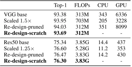
Table 4.Results of CNN Re-design by AOFP.
Top-1 FLOPs CPU GPU
VGG base 93.38 313M 343 6336
Scaled1.5× 93.95 703M 205 3228
Re-design-pruned 94.03 312M 351 8099
Re-design-scratch 93.69 312M -
-Res50 base 75.34 3.85G 14.4 437
Scaled1.25× 76.60 5.28G 11.2 353
Re-design-pruned 76.47 3.83G 14.2 430
Re-design-scratch 76.30 3.83G -
-budgets. To this end, we first train a scaled network from scratch and then apply AOFP until its FLOPs are reduced to the same level as the original model. In this way, we obtain a network where some layers are wider than the original architecture and some are narrower, so we call this process CNN Re-design. Concretely, we first scale the width of VGG and ResNet-50 (only the internal layers) by1.5× and1.25×, respectively, and apply AOFP using the same hyper-parameters as Sect.4.2. Though the pruned models outperform the baselines by a clear margin (Table.4), we still need to figure out whether the improvement is due to the better structure or the parameters initialized using the scaled model, so a counterpart with the same structure is trained from scratch, which delivers an accuracy higher than the baseline but lower than the pruned model. In this way, we safely claim the superiority of our optimized models over the tidy baselines. We present the discovered structures in the appendix to encourage further studies.
5. Conclusion
[image:9.612.319.532.213.321.2]Acknowledgement
This work was supported by the National Key R&D Pro-gram of China (No. 2018YFC0807500), National Natu-ral Science Foundation of China (No. 61571269), Na-tional Postdoctoral Program for Innovative Talents (No. BX20180172), and the China Postdoctoral Science Founda-tion (No. 2018M640131). We sincerely thank the reviewers for their comments.
References
Abbasi-Asl, R. and Yu, B. Structural compression of convo-lutional neural networks based on greedy filter pruning.
arXiv preprint arXiv:1705.07356, 2017.
Alvarez, J. M. and Salzmann, M. Learning the number of neurons in deep networks. In Advances in Neural Information Processing Systems, pp. 2270–2278, 2016.
Anwar, S., Hwang, K., and Sung, W. Structured pruning of deep convolutional neural networks.ACM Journal on Emerging Technologies in Computing Systems (JETC), 13(3):32, 2017.
Castellano, G., Fanelli, A. M., and Pelillo, M. An iterative pruning algorithm for feedforward neural networks.IEEE transactions on Neural networks, 8(3):519–531, 1997.
Collobert, R. and Weston, J. A unified architecture for natu-ral language processing: Deep neunatu-ral networks with mul-titask learning. InProceedings of the 25th international conference on Machine learning, pp. 160–167. ACM, 2008.
Deng, J., Dong, W., Socher, R., Li, L.-J., Li, K., and Fei-Fei, L. Imagenet: A large-scale hierarchical image database. InComputer Vision and Pattern Recognition, 2009. CVPR 2009. IEEE Conference on, pp. 248–255. IEEE, 2009.
Ding, X., Ding, G., Han, J., and Tang, S. Auto-balanced fil-ter pruning for efficient convolutional neural networks. In
Thirty-Second AAAI Conference on Artificial Intelligence, 2018.
Ding, X., Ding, G., Guo, Y., and Han, J. Centripetal sgd for pruning very deep convolutional networks with compli-cated structure. arXiv preprint arXiv:1904.03837, 2019.
GoogLe. Tensorflow-alexnet. https://github. com/tensorflow/models/blob/master/
research/slim/nets/alexnet.py, 2017a.
GoogLe. Tensorflow-slim. https://github. com/tensorflow/models/tree/master/
research/slim, 2017b.
Guo, Y., Yao, A., and Chen, Y. Dynamic network surgery for efficient dnns. InAdvances In Neural Information Processing Systems, pp. 1379–1387, 2016.
Han, S., Mao, H., and Dally, W. J. Deep compres-sion: Compressing deep neural networks with pruning, trained quantization and huffman coding.arXiv preprint arXiv:1510.00149, 2015a.
Han, S., Pool, J., Tran, J., and Dally, W. Learning both weights and connections for efficient neural network. In
Advances in Neural Information Processing Systems, pp. 1135–1143, 2015b.
Hassibi, B. and Stork, D. G. Second order derivatives for network pruning: Optimal brain surgeon. InAdvances in neural information processing systems, pp. 164–171, 1993.
He, K., Zhang, X., Ren, S., and Sun, J. Deep residual learn-ing for image recognition. InProceedings of the IEEE conference on computer vision and pattern recognition, pp. 770–778, 2016.
He, Y., Zhang, X., and Sun, J. Channel pruning for ac-celerating very deep neural networks. InInternational Conference on Computer Vision (ICCV), volume 2, pp. 6, 2017.
Hinton, G., Vinyals, O., and Dean, J. Distilling the knowledge in a neural network. arXiv preprint arXiv:1503.02531, 2015.
Hu, H., Peng, R., Tai, Y.-W., and Tang, C.-K. Net-work trimming: A data-driven neuron pruning approach towards efficient deep architectures. arXiv preprint arXiv:1607.03250, 2016.
Huang, Q., Zhou, K., You, S., and Neumann, U. Learning to prune filters in convolutional neural networks.arXiv preprint arXiv:1801.07365, 2018.
Ioffe, S. and Szegedy, C. Batch normalization: Accelerating deep network training by reducing internal covariate shift. InInternational Conference on Machine Learning, pp. 448–456, 2015.
Jaderberg, M., Vedaldi, A., and Zisserman, A. Speeding up convolutional neural networks with low rank expansions.
arXiv preprint arXiv:1405.3866, 2014.
Krizhevsky, A. and Hinton, G. Learning multiple layers of features from tiny images. 2009.
LeCun, Y., Boser, B. E., Denker, J. S., Henderson, D., Howard, R. E., Hubbard, W. E., and Jackel, L. D. Hand-written digit recognition with a back-propagation network. InAdvances in neural information processing systems, pp. 396–404, 1990a.
LeCun, Y., Denker, J. S., and Solla, S. A. Optimal brain damage. InAdvances in neural information processing systems, pp. 598–605, 1990b.
LeCun, Y., Bengio, Y., et al. Convolutional networks for images, speech, and time series. The handbook of brain theory and neural networks, 3361(10):1995, 1995.
Li, H., Kadav, A., Durdanovic, I., Samet, H., and Graf, H. P. Pruning filters for efficient convnets. arXiv preprint arXiv:1608.08710, 2016.
Liu, Z., Li, J., Shen, Z., Huang, G., Yan, S., and Zhang, C. Learning efficient convolutional networks through net-work slimming. In2017 IEEE International Conference on Computer Vision (ICCV), pp. 2755–2763. IEEE, 2017.
Luo, J.-H. and Wu, J. Autopruner: An end-to-end trainable filter pruning method for efficient deep model inference.
arXiv preprint arXiv:1805.08941, 2018.
Luo, J.-H., Wu, J., and Lin, W. Thinet: A filter level pruning method for deep neural network compression. In Proceed-ings of the IEEE international conference on computer vision, pp. 5058–5066, 2017.
Luo, J.-H., Zhang, H., Zhou, H.-Y., Xie, C.-W., Wu, J., and Lin, W. Thinet: pruning cnn filters for a thinner net. IEEE transactions on pattern analysis and machine intelligence, 2018.
Molchanov, D., Ashukha, A., and Vetrov, D. Variational dropout sparsifies deep neural networks. In Proceed-ings of the 34th International Conference on Machine Learning-Volume 70, pp. 2498–2507. JMLR. org, 2017.
Molchanov, P., Tyree, S., Karras, T., Aila, T., and Kautz, J. Pruning convolutional neural networks for resource efficient inference. 2016.
Mozer, M. C. and Smolensky, P. Using relevance to reduce network size automatically. Connection Science, 1(1): 3–16, 1989.
Polyak, A. and Wolf, L. Channel-level acceleration of deep face representations.IEEE Access, 3:2163–2175, 2015.
Roth, V. and Fischer, B. The group-lasso for generalized linear models: uniqueness of solutions and efficient algo-rithms. InProceedings of the 25th international confer-ence on Machine learning, pp. 848–855. ACM, 2008.
Sharma, A., Wolfe, N., and Raj, B. The incredible shrink-ing neural network: New perspectives on learnshrink-ing rep-resentations through the lens of pruning. arXiv preprint arXiv:1701.04465, 2017.
Simonyan, K. and Zisserman, A. Very deep convolu-tional networks for large-scale image recognition.arXiv preprint arXiv:1409.1556, 2014.
Srivastava, N., Hinton, G. E., Krizhevsky, A., Sutskever, I., and Salakhutdinov, R. Dropout: a simple way to prevent neural networks from overfitting. Journal of machine learning research, 15(1):1929–1958, 2014.
Wang, H., Zhang, Q., Wang, Y., and Hu, H. Structured probabilistic pruning for convolutional neural network acceleration.arXiv preprint arXiv:1709.06994, 2017a.
Wang, Y., Xu, C., You, S., Tao, D., and Xu, C. Cnnpack: Packing convolutional neural networks in the frequency domain. InAdvances in neural information processing systems, pp. 253–261, 2016.
Wang, Y., Xu, C., Xu, C., and Tao, D. Beyond filters: Com-pact feature map for portable deep model. In Interna-tional Conference on Machine Learning, pp. 3703–3711, 2017b.
Wen, W., Wu, C., Wang, Y., Chen, Y., and Li, H. Learn-ing structured sparsity in deep neural networks. In Ad-vances in Neural Information Processing Systems, pp. 2074–2082, 2016.
Xu, K., Wang, X., Jia, Q., An, J., and Wang, D. Globally soft filter pruning for efficient convolutional neural networks. 2018.
Ye, J., Lu, X., Lin, Z., and Wang, J. Z. Rethinking the smaller-norm-less-informative assumption in chan-nel pruning of convolution layers. arXiv preprint arXiv:1802.00124, 2018.
Yu, R., Li, A., Chen, C.-F., Lai, J.-H., Morariu, V. I., Han, X., Gao, M., Lin, C.-Y., and Davis, L. S. Nisp: Pruning networks using neuron importance score propagation. In
Proceedings of the IEEE Conference on Computer Vision and Pattern Recognition, pp. 9194–9203, 2018.