VIS3COS I:Survey overview and the role of environment and stellar mass on star formation

May 22, 2018

VIS

3

COS: I. survey overview and the role of environment and

stellar mass on star formation

?

Ana Paulino-Afonso

, David Sobral

, Behnam Darvish

, Bruno Ribeiro

, Andra Stroe

, Philip Best

,

José Afonso

, and Yuichi Matsuda

1 _{Instituto de Astrofísica e Ciências do Espaço, Universidade de Lisboa, OAL, Tapada da Ajuda, PT1349-018 Lisboa, Portugal} 2 _{Departamento de Física, Faculdade de Ciências, Universidade de Lisboa, Edifício C8, Campo Grande, PT1749-016 Lisboa,}

Portu-gal

3 _{Department of Physics, Lancaster University, Lancaster, LA1 4YB, UK}

4 _{Leiden Observatory, Leiden University, P.O. Box 9513, NL-2300 RA Leiden, The Netherlands}

5 _{Cahill Center for Astrophysics, California Institute of Technology, 1216 East California Boulevard, Pasadena, CA 91125, USA} 6 _{Centro de Computação Gráfica, CVIG, Campus de Azurém, PT4800-058 Guimarães, Portugal}

7 _{European Southern Observatory, Karl-Schwarzschild-Str. 2, 85748, Garching, Germany}

8 _{Institute for Astronomy, University of Edinburgh, Royal Observatory, Blackford Hill, Edinburgh EH9 3HJ, UK} 9 _{National Astronomical Observatory of Japan, Osawa 2-21-1, Mitaka, Tokyo 181-8588, Japan}

ABSTRACT

We present the VIMOS Spectroscopic Survey of a Supercluster in the COSMOS field (VIS3COS) at z ∼ 0.84. We use VIMOS high resolution spectra (GG475 filter) to spectroscopically select 490 galaxies in and around the superstructure and an additional 481 galaxies in the line of sight. We present the redshift distribution, the catalogue to be made public, and the first results on the properties of individual galaxies and stacked spectra (3500Å< λ <4200Å rest-frame). We probe a wide range of densities and environments (from low-density field to clusters and rich groups). We find a decrease in the median star formation rate from low to high-density environments in all bins of stellar mass and a sharp rise of the quenched fraction (from∼10% to∼40−60%) of intermediate stellar mass galaxies(10 <log₁₀(M?/M) < 10.75)from filaments to clusters. The quenched fraction for massive galaxies shows little

dependence on environment being constant at∼30−40%. We find a break in the strength of the [OII] emission, with nearly constant line equivalent widths at lower densities (∼ −11Å) and then a drop to∼ −2.5Å towards higher densities. The break in the [OII] line strength happens at similar densities (log₁₀(1+δ) ∼0.0−0.5) as the observed rise in the quenched fraction. Our results may provide further clues regarding the different environmental processes affecting galaxies with different stellar masses and highlight the advantages of a single dataset in the COSMOS field probing a wide range of stellar masses and environments. We hypothesize that quenching mechanisms are enhanced in high density regions.

Key words. galaxies: clusters – galaxies: evolution – galaxies: high redshift – large-scale structure of Universe

1. Introduction

In the local Universe, we observe differences in a wide range of galaxy properties (e.g. colours, star formation, morphology) with respect to the environment they reside in (e.g.Oemler 1974; Dressler 1980,1984). Cluster galaxies are typically red and pas-sive, while in low-density environments the population is domi-nated by blue star-forming galaxies (e.g.Dressler 1980;Balogh et al. 2004; Kauffmann et al. 2004; Baldry et al. 2006; Bam-ford et al. 2009). The star formation rate (SFR) and star-forming fraction (fSF) have also been found to correlate strongly with the projected galaxy density (e.g. Lewis et al. 2002; Gómez et al. 2003;Hogg et al. 2004;Best 2004;Kodama et al. 2004;Peng et al. 2010; Darvish et al. 2016;Cohen et al. 2017). Observa-tions also imply that the most massive galaxies assembled their stellar mass more quickly and had their bulk of star formation

? _{Based on observations obtained with VIMOS on the ESO/VLT}

un-der the programmes 086.A-0895, 088.A-0550, and 090.A-0401.

?? _{E-mail: [email protected]} ??? _{ESO fellow}

quenched atz & 1(e.g.Iovino et al. 2010). While stellar mass and environmental density correlate, it is now possible to disen-tangle their roles and show that both are relevant for quenching star formation (e.g.Peng et al. 2010;Sobral et al. 2011;Muzzin et al. 2012;Darvish et al. 2016).

Globally, observations show that the star formation rate den-sity (ρSFR) peaks at z ∼ 2 −3 and has been declining ever since (e.g.Lilly et al. 1996;Karim et al. 2011;Burgarella et al. 2013; Sobral et al. 2013; Madau & Dickinson 2014; Khosto-van et al. 2015). However, surprisingly, the decline ofρSFRwith increasing cosmic time is happening in all environments (e.g. Cooper et al. 2008;Koyama et al. 2013). Recent studies have also shed more light on when the dependency of star-forming galaxies on environment start to become observable (e.g. Scov-ille et al. 2013;Darvish et al. 2016). However, it is still unclear exactly how the environment affected the evolution of galaxies and how that may have changed across time. In order to properly answer such questions it is mandatory to conduct observational surveys at high redshift (e.g.Tadaki et al. 2012;Koyama et al. 2013;Lemaux et al. 2014;Cucciati et al. 2014;Shimakawa et al.

2018) which can then be used to test theoretical models of galaxy evolution (e.g.Vogelsberger et al. 2014;Genel et al. 2014; Hen-riques et al. 2015;Schaye et al. 2015;Crain et al. 2015).

There have been a plethora of surveys of clusters and their surroundings atz .1(e.g.Treu et al. 2003;Cooper et al. 2008; Poggianti et al. 2009;Lubin et al. 2009;Cucciati et al. 2010b; Iovino et al. 2010;Li et al. 2011;Muzzin et al. 2012;Mok et al. 2013;Koyama et al. 2013;Lemaux et al. 2014; Cucciati et al. 2014,2017) with a key focus on the influence of environment on the star formation of galaxies. Emission line surveys of clus-ters at lower redshifts (z∼0.1−0.5) targeting either Hα(e.g. Balogh et al. 2002;Stroe & Sobral 2015;Stroe et al. 2017; So-bral et al. 2016; Rodríguez del Pino et al. 2017) or [OII] (e.g. Nakata et al. 2005) find that star formation is suppressed in clus-ter environments. This suppression seems to be more effective for early-type galaxies (e.g.Balogh et al. 2002) and to be a slow acting mechanism that mainly affects the gas component (e.g. Rodríguez del Pino et al. 2017).

Byz∼1, some authors have claimed to have found a flatten-ing, or even a definitive reverse, of the relation between the star formation activity and the projected local density, either study-ing how the average SFRs of galaxies change with local density (Elbaz et al. 2007) or looking at fSFas a function of density (e.g. Ideue et al. 2009;Tran et al. 2010;Santos et al. 2014). These results would be naturally interpreted as a sign of evolution if other studies (e.g.Patel et al. 2009;Sobral et al. 2011;Muzzin et al. 2012;Santos et al. 2013) had not found an opposite re-sult. The differences found between different clusters may be related to their dynamical state, as merging clusters in the low-redshift Universe can also show reverse trends when compared to relaxed clusters at similar epochs (e.g.Stroe et al. 2014,2015, 2017; Mulroy et al. 2017), but other factors like sample size, AGN contamination, environments probed may also play a role (e.g.Darvish et al. 2016).Sobral et al.(2011), probing a wide range of environments and stellar masses, were able to recover and reconcile the previous apparently contradictory results. They attribute the discrepancies to selection effects. If one restricts to similar stellar masses and/or densities we can find similar trends in different studies.Sobral et al.(2011) also separated the indi-vidual roles of mass and environment in galaxy evolution (see alsoIovino et al. 2010;Cucciati et al. 2010a;Peng et al. 2010; Li et al. 2011).

Finding the exact mechanisms of galaxy quenching and their physical agents is still one of the unsolved problems in galaxy evolution. Many internal (e.g. stellar and AGN feedback) and external (e.g. galaxy environment) physical drivers are thought to be linked to the quenching process. One might naively expect a continuous decline in the star formation of galaxies from the field to the dense cores of clusters (e.g. due to a lower amount of available gas or faster gas consumption as galaxies move trough denser mediums). However, before galaxies undergo a full quenching process in dense regions, they may experience a temporary enhancement in star formation activity (see e.g. So-bral et al. 2011) which may complicate how observations are interpreted (e.g. ram pressure stripping - Gallazzi et al. 2009; Bekki 2009; Owers et al. 2012; Roediger et al. 2014- and/or tidal interactions -Mihos & Hernquist 1996;Kewley et al. 2006; Ellison et al. 2008).

When looking in more detail at galaxies in the low to in-termediate redshift Universe (z . 1), many properties of star-forming galaxies that are directly or indirectly linked to star formation activity (e.g. SFR, sSFR, emission line equivalent widths and the main-sequence of star-forming galaxies) seem to be invariant to their environment (but it is still a debated issue,

see e.g.Peng et al. 2010; Iovino et al. 2010; Wijesinghe et al. 2012;Muzzin et al. 2012;Koyama et al. 2013,2014; Hayashi et al. 2014; Darvish et al. 2014, 2015a, 2016). Therefore, the main role of the environment seems to be to set the fraction of quiescent/star-forming galaxies (e.g.Peng et al. 2010;Cucciati et al. 2010a;Sobral et al. 2011;Muzzin et al. 2012;Darvish et al. 2014,2016) which is likely linked to the reported a gas deficit in cluster galaxies (seen in atomic hydrogen, e.g.Giovanelli & Haynes 1985;Cortese et al. 2010;Serra et al. 2012;Brown et al. 2017). But this is not the picture found when looking at molec-ular hydrogen which is either independent of environment, de-pressed or enhanced in high density regions dependent on the study (e.g.Boselli et al. 2014;Mok et al. 2016; Koyama et al. 2017). Nevertheless, recent studies are finding that not all char-acteristics of star-forming galaxies are independent of environ-ment. For example, metallicities have been shown to be a func-tion of environment (e.g. Kulas et al. 2013; Shimakawa et al. 2015;Sobral et al. 2015) with studies finding that star-forming galaxies have slightly higher metallicities in high density ronments when compared to lower density/more typical envi-ronments atz∼0.2−0.5(e.g.Sobral et al. 2015;Darvish et al. 2015a).Sobral et al.(2015) study a cluster undergoing a merger andDarvish et al.(2015a) focus on galaxy filaments which are both regions of enhanced dynamical activity. Denser environ-ments also seem to boost the dust content of star-forming galax-ies (e.g.Koyama et al. 2013;Sobral et al. 2016). The higher dust content seen in high density regions can be a requirement for galaxies to sustain star formation in such environments, by al-lowing for dense and compact regions to survive environmental stripping.

Issues related to photometric redshift errors and projection effects can limit our understanding of what is occurring in and around clusters. These issues dilute genuine trends and prohibit us from unveiling the role of the environment in sufficient de-tail to really test our understanding. Surveys such as EDisCS (e.g.White et al. 2005) have aimed to overcome some of these issues by targeting the densest regions at high redshift with ex-tensive spectroscopic observations. These have made significant progress (Poggianti et al. 2006, 2009; Cucciati et al. 2010a, 2017), but either they target deep and small areas or shallow and wide areas. This limits the study on the role of the larger-scale structure and the densest environments simultaneously. A way to make further progress is to conduct a spectroscopic sur-vey (to avoid projection effects and photometric redshift biases and errors) over a superstructure containing the complete range of environments in a sub-deg2area at high redshift.

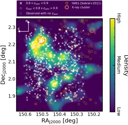
Fig. 1.Snapshot of the region targeted by our spectroscopic survey. The colormap encodes the information on the galaxy projected surface density at the redshift slice of interest at0.8 < z < 0.9estimated from the catalogue made public byDarvish et al.(2017). Each thick white cross represents a targeted galaxy with a measured spectroscopic redshift in the same redshift slice. The white pentagons show a targeted galaxy with measured spectroscopic redshift, outside the defined redshift slice. The blue circles show the targeted galaxies for which we have not a measured spectroscopic redshift. The orange squares show the location of Hαemitters studied bySobral et al.(2011). The large red circles denote the location of X-ray detected clusters fromFinoguenov et al.(2007) at the same redshifts. The size of the circle shows the cluster estimated X-ray radiusr500.

We see here that we are probing a large range of densities with our survey, in part due to selection effects (e.g. slit placement constraints).

2. Sample and observations

2.1. The COSMOS superstructure atz≈0.84

By conducting a relatively wide (∼0.8square degrees) and deep (down to a flux limit of8×10−17_{erg s}−1_cm−2_{) Hαsurvey atz=}

0.84in the COSMOS field,Sobral et al.(2011) found a strikingly large overdensity of Hαemitters within a region that happens to contain 3 X-ray clusters (first reported in Finoguenov et al. 2007), as shown in Figure1. Limited spectroscopic observations

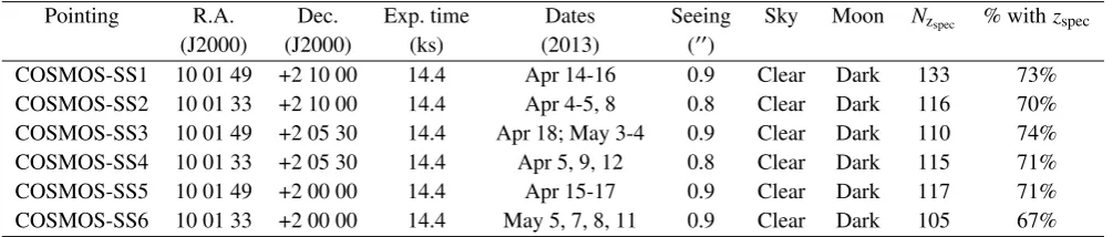
Table 1.Observing log for our observations with VIMOS on the VLT for programmes 086.A-0895, 088.A-0550, and 090.A-0401 (PI: Sobral). The last two columns show the number of targeted objects for each pointing with a spectroscopic redshift and the spectroscopic success rate, respectively.

Pointing R.A. Dec. Exp. time Dates Seeing Sky Moon Nzspec % withzspec

(J2000) (J2000) (ks) (2013) (00)

COSMOS-SS1 10 01 49 +2 10 00 14.4 Apr 14-16 0.9 Clear Dark 133 73%

COSMOS-SS2 10 01 33 +2 10 00 14.4 Apr 4-5, 8 0.8 Clear Dark 116 70%

COSMOS-SS3 10 01 49 +2 05 30 14.4 Apr 18; May 3-4 0.9 Clear Dark 110 74%

COSMOS-SS4 10 01 33 +2 05 30 14.4 Apr 5, 9, 12 0.8 Clear Dark 115 71%

COSMOS-SS5 10 01 49 +2 00 00 14.4 Apr 15-17 0.9 Clear Dark 117 71%

COSMOS-SS6 10 01 33 +2 00 00 14.4 May 5, 7, 8, 11 0.9 Clear Dark 105 67%

Table 2.Properties of the clusters in and around the VIMOS target fields (see Figure1). The cluster coordinates are from the catalogue produced byFinoguenov et al.(2007). The other properties were computed byBalogh et al.(2014). The third column is the median redshift of galaxy members. The fourth column is the intrinsic velocity dispersion. The fifth and sixth columns are thermsprojected distance of all group members from the centre and corresponding mass of the cluster, respectively.

Label R.A. Dec. z σi Rrms Mrms

(J2000) (J2000) (km/s) (Mpc) (1013_M

)

A 150.505 2.224 0.84 560±60 0.81±0.07 17.4±5.9

B 150.370 1.999 0.83 420±40 0.34±0.03 4.2±1.3

C 150.211 2.281 0.88 680±70 0.23±0.03 7.5±2.8

the opportunity to study such a range of environments in a single data-set, we have designed a spectroscopic survey over this full region.

2.2. Target selection

In order to accurately map the 3D large-scale structure at z =

0.84and identify the bulk of cluster, group, filament, and field members, we have targeted member candidates (using the VI-MOS Mask Preparation Software to maximize the number of targets per mask) down to I = 22.5 (corresponding to stellar masses of ≈1010_M

for older and passive galaxies but much

lower for younger galaxies, which have lower M/L ratios - see e.g.Sobral et al. 2011). Our targets are selected by using state-of-the-art photometric redshifts (photo-zs) in COSMOS, using up to 30 narrow, medium, and broad bands (c.f. Ilbert et al. 2009). In practice, we use the upper and lower limits of the 99% photo-zconfidence interval and select all sources for which such interval overlaps with0.8 < z < 0.9 (including sources best-fit by a quasar/AGN template). We reject all sources that are likely to be stars by excluding those sources for which χ2_(star)/χ2_{(galaxy) < 0.2(c.f.Ilbert et al. 2009) or with clear} star-like morphologies in high-resolution HST imaging and pre-senting near-IR vs. optical colours, which clearly classifies them as stars (following e.g.Sobral et al. 2013).

In order to effectively fill the masks, we introduce galaxies down to I = 23.0 and with photo-zs of0.6 < z < 1.1. We note that we use the 99% photo-z confidence interval instead of the best photo-zto avoid significant bias towards redder and older galaxies (as blue and younger galaxies tend to present the largest scatter in the photometric versus spectroscopic redshift comparison). We also note that this selection recovers all our blue and star-forming Hα emitters (Sobral et al. 2009,2011). We can therefore fully map the supercluster without major se-lection biases. In total, out of our entire parent sample of 1015 primary targets and 2257 secondary targets, we have placed 531 (∼55% of the parent primary) slits on primary targets and 440

(∼19% of the parent secondary) on secondary targets. Due to the six pointings targeting the same area we are not substantially bi-ased against targets in higher densities (see also SectionA). Ob-servations are described in Section2.3. We discuss our sample completeness in terms of spectroscopic success and relative to our parent sample in AppendixAand apply corrections when-ever completeness effects might bias our results (see example Section4.2).

2.3. Observations

We have targeted the COSMOS superstructure identified in So-bral et al. (2011) and studied photometrically in e.g.Darvish et al.(2014). We have used the High Resolution Red grism (HR-Red) with VIMOS (Le Fèvre et al. 2003) and the GG475 filter1. Our observations are summarized in Table2and probe the rest-frame3400−4600Å for our main targets (atz ∼ 0.8) with an observed 0.6 Å pix−1spatial scale, which atz∼0.8is∼0.33Å pix−1 rest-frame. This allows for a clear separation of the spec-tral features and very accurate redshift determinations. Spectra cover a key spectral range atz ≈0.84, from [OII]λ3726,λ3729 (partially resolving the doublet, as our resolution is∼ 1Å for

z∼0.8sources) through 4000 Å (allowing us to measure D4000, see Figure2) to beyond Hδat high resolution (allowing to mea-sure many other absorption lines and obtain their width).

The observations cover a contiguous overdense region of

210×310(9.6×14.1Mpc, see Figure1) using 6 VIMOS pointings (chosen to overlap in order to assure both a contiguous coverage and a good target coverage and completeness, particularly for sources located in the densest regions). We have used the VI-MOS 100width slit with an average of 900slit length. Our setup allowed us to offset different observing blocks by±1.300along the slit to guarantee an optimal sky subtraction. Observations were conducted in service mode in April and May 2013 (see

Fig. 2.Three individual examples of images and spectra obtained with our survey. Each thumbnail (left panel) shows the HST/ACS F814W image of each target from the COSMOS survey (Koekemoer et al. 2007) with the VIMOS slit overlaid (dashed yellow line). To the right of each stamp we show the corresponding 2D (top) and 1D (bottom) spectrum. We mark with vertical dashed lines the position of some spectral features present in our spectra.

ble1) under clear conditions, new moon and an average seeing of 0.900(ranging from 0.600 to 0.9500). Our pointings, labelled COSMOS-SS1 through COSMOS-SS6, have a total exposure of 4 hours each. Arcs and flats were taken each night. See Table1 for further details.

2.4. Data reduction

Data reduction was done using the VIMOS ESO pipeline, ver-sion 6.10, through gasgano2. The reduction is performed quad-rant by quadquad-rant (VIMOS has 4 different quadquad-rants, labelled Q1 through to Q4). First, a master bias per night of observations is created by median combining bias frames per quadrant. Appro-priate recipes are run in order to create master flats and master arcs for wavelength calibration. The pipeline is used to flag and mask hot pixels and cosmic rays and also to distort correct the observations. We obtain a sky subtracted spectra by estimating the median sky emission in several apertures away from each extracted source. Finally, 2D spectra are obtained by combining spectra obtained over different observing blocks. The extraction of the 1D spectra is conducted by collapsing the spectra in wave-length and then extracting along the trace’s FWHM. We obtain our 2D and 1D spectra with a relative flux calibration. We are able to extract 1D spectra for 971 sources, with varying levels of S/N. See Figure2for examples of individual 1D and 2D spectra.

2.5. Flux calibration

Due to the wealth of available well-calibrated photometry for all our sources, we use broad and medium band data from COS-MOS to test and then scale the flux calibration of our spectra. This allows us to obtain more accurate flux calibrations and to slit correct more appropriately than using a single standard star

2 http://www.eso.org/sci/software/gasgano.html

for each quadrant. This also allows us to correct for any mis-alignment in the slit position relative to each source.

Briefly, we use the I-band selected photometric catalogue presented byIlbert et al. (2009) and start by using the I-band magnitudes. We convert I-band magnitudes into flux densities for each of our targets and compare those with the integral of the spectra convolved with theI-band filter. We then scale each spectra by the appropriate flux normalisation such that the inte-gral within theI-band filter equals the flux density derived from photometry. Note that it also allows us to obtain a relatively good slit correction and thus we do not apply any further slit correc-tions for our data. For galaxies which are too faint in theI-band, we use the median flux calibration for the pointing and quadrant it was observed in. This flux calibration is done under the as-sumption that galaxies have an homogeneous colour over their extent.

As a further check, we also use the COSMOS medium band flux densities (see e.g.Ilbert et al. 2009) and check that our flux calibration is valid for the full range of available medium bands. We find very good agreement at all wavelengths within±10−

15% which we interpret as our uncertainty in the flux calibration.

2.6. Redshift measurements

red-Fig. 3. Spectroscopic redshift distribution of the galaxies targeted in our sample as a black histogram. The vertical black dashed lines de-limit the redshift selection of the results presented in this paper. The red line shows our Gaussian fit to the distribution without using rejec-tion algorithms, pinpointingz=0.836±0.008as the core redshift of the densest structure we find. The peak at slightly higher redshift (z∼0.88) is likely produced members from the north-western cluster C (see Table

2and Figure1).

shifts for 696 sources with high S/N. The redshift distribution for the galaxies in our sample is shown in Figure3.

2.7. Final sample

Our final sample is restricted to be at0.8 < z < 0.9 to match our primary selection (see Section 2.2) and has a total of 490 galaxies spanning a large diversity of environments across sev-eral Mpc that contain 3 X-ray confirmed galaxy clusters. We are releasing the final catalogue with this paper and we show in Ta-bleB.1the first 10 entries.

3. Determination of galaxy properties

3.1. Measurement of [OII]λ3726,λ3729 line

To obtain flux measurements of emission lines from our spectra, we interactively iterate through the entire dataset and zoom to a window of100Å around [OII]λ3726,λ3729. We define two regions of∼15Å (one blueward, one redward of the line) from which we estimate the median continuum level. Then the local continuum is defined as a straight line that goes through those points. To fit the doublet we use a combination of two Gaussian models through the functional form:

f(λ)=A1exp

−(λ−λ1) 2

2σ2

+A2exp

−(λ−λ2) 2

2σ2

, (1)

with 3 free parameters: A1,A2, andσ. The parameters A1 and

A2are the amplitudes of each component,σis the width of each Gaussian component. The centre of each component is fixed to beλ1=3726.08±0.3Å andλ2 =3728.88±0.3Å (we allow for a small shift in the line centre that is of the size of the resolu-tion element of the spectra). To estimate the line properties we use the information on the error spectra and perturb each flux at all wavelengths considered for the fitting by drawing a random number on the observed value and with a width that is equal to

Fig. 4.Stellar masses and star formation rates derived from SED fit-ting (see Section3.2) in our spectroscopic sample at0.8<z<0.9. For comparison we show the derived best-fit relation for star-forming galax-ies computed atz=0.84using the equation derived byWhitaker et al.

(2012) over a large average volume in the COSMOS field. The verti-cal dotted line shows the completeness limit of our survey. The dotted contours show the COSMOS2015 (Laigle et al. 2016) distribution of galaxies with0.8<zphot<0.9andiAB<23from 10% to 95% of the

sample in 5% steps. Empty circles highlight the photometric quiescent sample withlog₁₀(sSF R)<−11.

its error. We run this exercise 10000 times and then estimate the errors on the line fit by taking the 16th and 84th percentile of the distribution in each free parameter.

From now on we only use individual measurements if the S/N is>3. We note that in Section3.4we will obtain and mea-sure stacks as a function of environment, allowing us to obtain the median properties of spectral lines for specific subsets of galaxies irrespective of their individual detection. This of course leads to a much higher S/N. We measure the line properties of the stacks with the same procedure described here for individual sources.

3.2. Stellar masses and star formation rates

compare our results on stellar mass and star formation rates with those provided in the COSMOS2015 catalogue and find a dis-persion of ∼0.3dex for the stellar mass and∼0.7dex for the SFRs.

We present in Figure4 the stellar masses and star forma-tion rates in our sample and show that we are probing galax-ies withlog₁₀(M?/M) & 9 in a wide range of SFRs (−2 .

log₁₀(SF R).2). We see that our sample includes normal star-forming galaxies as well as galaxies that are found well below the SFR main sequence (see e.g.Noeske et al. 2007;Elbaz et al. 2007;Whitaker et al. 2012), which are characteristic of galax-ies in the process of star formation quenching or just quenched (e.g.Fumagalli et al. 2014). To select quiescent galaxies within our sample we impose a specific SFR cut atlog₁₀(sSF R)<−11

(see e.g.Ilbert et al. 2010;Carollo et al. 2013) and find a total of 64 galaxies in these conditions.

We also obtain from MAGPHYS the effective optical depth of the dust in theV-band,τV, which we translate into an average reddening value ofE(B−V)=1.086τV/RV(assumingRV =3.1, see e.g.Draine 2004). We find that our galaxies have an average reddening value of E(B −V) ∼ 0.27±0.02. We report here that abovelog10(M?/M)&10there is little dependence of the median extinction with stellar mass with a reddening value of

E(B−V) ∼ 0.32±0.02 (∼ 0.37±0.02 if we consider star-forming only).

We measure the [OII] line flux by integrating over the best fit model described by Eq.1, which can be solved analytically as

F=σ

√

2π(A1+A2). We correct the measured [OII] luminosity by the SED extinction value. The corrected luminosity is given by

L[OII],corr=L[OII]/e−τ[OII], (2)

whereτ[OII]is the optical depth atλ=3727Å derived using the

dust model used inMAGPHYS (CHARLOT& FALL2000). The effect of extinction on the luminosity of [OII] is displayed on Figure5and it can account for the difference that we find when comparing SED and [OII] SFRs using the calibration derived by Kewley et al.(2004) and applying a conversion factor between Salpeter(1955) andChabrier(2003) IMFs:

SF R= 6.58×10

−42

1.7 L[OII],corr. (3)

We find a spread of 0.64 dex but on average the derived SFRs are consistent with each other (median difference of 0.07 dex). We also show the SFR as derived from Hαluminosity (Kennicutt 1998) from the HiZELS survey, which was used to first pinpoint the existence of this structure (Sobral et al. 2011).

We stress however that [OII] emission can originate from other sources not related to star formation (e.g. AGN, LINERs) and that it is a poor tracer of SFR for red galaxies (e.g.Yan et al. 2006;Kocevski et al. 2011). This tracer is also dependent on the metallicity of the galaxy (Kewley et al. 2004). Those are the rea-sons for our choice to do our analysis in terms of star formation in galaxies using the quantity derived from SED fitting instead of relying on [OII] emission as a tracer of SFR.

3.3. Overdensities estimation

The estimate of local overdensity was computed as described by Darvish et al. (2015b,2017) and is based on the photometric redshift catalogue of the COSMOS survey presented by Ilbert

Fig. 5.SFR estimates from SED fitting and from [OII] (derived from equation 4 ofKewley et al. 2004) of the galaxies in our spectroscopic sample at0.8<z <0.9. As red circles we show the dust uncorrected Hαderived star formation rates for the galaxies in our sample and that were measured bySobral et al.(2011). The subscriptcorrdenotes the dust corrected SFRs derived from each estimate using the optical depth derived through SED fitting (see Section3.2).

Fig. 6.Overdensity distribution for the galaxies in our sample with

0.8 < z < 0.9. We show the different cosmic web environments of galaxies (field, filament, and cluster) according to their classification using the scheme devised byDarvish et al.(2014,2017).

et al. (2013, see also Muzzin et al. 2013; Laigle et al. 2016). The density field was computed over an area of∼1.8 deg2 us-ing a mass-complete sample with accurate photometric redshifts spanning0.1<zphot<1.2. The surface density field was com-puted in 2D slices of redshift of widths ±1.5σ∆z/(1+z)(as

sug-gested byMalavasi et al. 2016). To properly account for the un-certainty on the photometric redshift estimate, the full photo-z

assigned to each point in the density field is (based on adaptive kernel smoothing):

Σ_i = 1 ÍN

i=1,wi N Õ

i=1,

wiK(®r,r®i,hi), (4)

wherer®is a location in the density field,r®iis the position of each galaxy,wiis the weight assigned to each galaxy,hiis the kernel width at the position of each galaxy, andKis a two-dimensional Gaussian kernel function.

In these equations,Nis the number of galaxies in the slice with weights greater than 10%,ri is the position of the galaxy,

rj is the position of all other galaxies in the slice, andhi is the adaptive smoothing parameter for our assumed kernel. The value of hi =h

p

G/Σ_i Mpc, whereΣ_i is the initial density estimation at the position of galaxyiusing a fixed kernel with of 0.5 Mpc width,Gis the geometric mean of allΣ_i at each redshift slice, and h is chosen to have a value around the typical size of X-ray clusters (0.5 Mpc, see e.g.Finoguenov et al. 2007). We then evaluate the density field in a 2D grid with a spatial resolution of 50 kpc at each redshift. We define overdensity as:

1+δ= Σ

Σ_median (5)

withΣ being the projected local density andΣmedian being the median of the density field of the redshift slice the galaxy is in. We choose to use number densities instead of mass density esti-mates (e.g.Wolf et al. 2009) to avoid introducing any bias due to any underlying relation between stellar mass and density that may exist. For a more detailed description of the method, we re-fer the reader toDarvish et al.(2014) andDarvish et al.(2015b). We have computed the value of the overdensity for each galaxy by interpolating the density field to their angular position and spectroscopic redshift. We show in Figure6the distribution of our galaxies according to their overdensity and labelled by the region they are likely to belong to, as defined by the cosmic web measurements computed byDarvish et al.(2014,2017). We note that when referring to galaxies within our spectroscopic sample in cluster regions we are mostly referring to either rich groups or the outskirts of massive clusters as our observational setup does not allow for a good sampling of densely populated regions due to slit collision problems.

We note that there is an overlap between the different la-belled regions and the measured local overdensity in Figure 6. This happens because the region assigned to each galaxy is based on the definition of the strength of the cluster and filament sig-nals, which takes into account the morphology of the density field. That is the reason why a pure density-based definition of the environment of galaxies cannot fully separate them into real physical structures (see e.g.Aragón-Calvo et al. 2010;Darvish et al. 2014). This means for example that we can have dense filaments (as high density regions with thread-like morphology, likely infall regions of massive clusters) and less dense cluster regions (intermediate density with circular morphology, likely associated with galaxy groups). We refer toDarvish et al.(2014, 2017see alsoAragón-Calvo et al. 2010) for more details.

3.4. Spectral stacks

To increase the S/N on the obtained spectra and investigate de-tails on the spectral properties of galaxies as a function of their

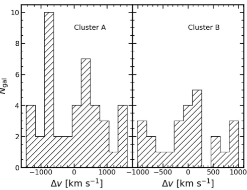
Fig. 7.The velocity distribution for clusters A (left) and B (right) of all member galaxies. We note that these structures cannot be described by a single Gaussian shape indicating that these structures are not virialized.

stellar mass and local density, we have performed stacking of individual galaxy spectra. Our stacking method can be summa-rized as a median, interpolated, and normalized spectra. For each set of spectra we start by shifting the spectrum to its rest-frame wavelengths using the redshift we have measured (see Section 2.6). Then we linearly interpolate the spectra onto a common universal grid (3250-4500 Å,∆λ = 0.3Å/pixel). We normalize each spectrum to the mean flux measured from 4150-4350 Å. Lastly, we median combine all spectra by taking the median flux at each wavelength. We estimate that our typical errors in the spectroscopic redshift measurements are on the order of ∼ 0.0005, which translates to an error of∼ 1 Å, comparable to our spectral resolution atz∼0.8. Thus, our stacking should not smear the lines enough to affect the measurements on the [OII]λ3726,λ3729 doublet.

4. Results

Throughout this section, our measure of environment is quanti-fied byδ(see Equation5). For a broad comparison between dif-ferent environments, we defined as lower density galaxies resid-ing inlog₁₀(1+δ)<0.1and as higher density galaxies residing in regions withlog10(1+δ)>0.4.

4.1. Redshift distribution

From our first redshift measurements, based on 2-3 lines and the dispersion of the measurements, we are able to derive the full redshift distribution of our VIMOS sample. We show the results in Figure3which shows a very clear peak atz≈0.84. By fitting a Gaussian to the redshift distribution atz≈0.8we find that the COSMOS superstructure is well characterised byz=0.84±0.01

with 367 galaxies fully included within this redshift distribution. We attempt to estimate the mass of the two clusters for which we have coverage (A and B on Table 2, see also Figure1) by computing the radial velocity dispersion,σr, of the spectroscop-ically confirmed galaxies in our sample. We estimate the size of the cluster by computing the root mean square of the distances,

a final estimate for each cluster, we iterate 5 times and compute the mean position,Rrms, andσrby selecting at each step galaxies within 2Rrmsof the cluster centre and within 2σof the median cluster redshift. We start our iteration procedure by assuming an initial guess forRrms=0.5Mpc.

We find values of σr = 875±179 km s−1 (43 galaxies) and Rrms = 1.1 Mpc for cluster A and of σr = 598 ±225 km s−1 (25 galaxies) and Rrms = 1.3 Mpc for cluster B. As-suming a virial state for each cluster, we can estimate their mass as M = 3σr2Rrms/G. We find M = 6±3×1014M and

M = 3±2×1014M, respectively. These values are up to an order of magnitude higher than the values reported by Balogh et al.(2014, see Table2) and this difference is mainly driven by our larger derived values of Rrms. We note here that our mea-surements are done under the assumption that the clusters are virialized. We hypothesize that when applying a similar criteria for galaxy membership as Balogh et al. (2014), we are likely picking up additional moving substructures (at slightly differ-ent redshifts) that are artificially increasing our measured clus-ter sizes and velocity dispersion. This is supported by the non-Gaussian shape of the velocity distribution histograms of the se-lected members (see Fig.7).

4.2. SFR dependence on local overdensity

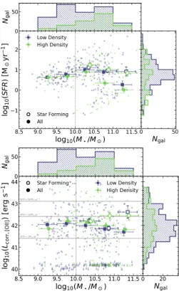
We show in the upper panel of Figure 8 the dependence of SFR on stellar mass and local density. For low mass galax-ies (log10(M?/M) . 10) we find the same average SFR in both high and low density regions, although there are only very few (∼10) low mass galaxies in our sample in high density re-gions and all of them are star-forming (check completeness in Figure A.1). At higher stellar masses (log₁₀(M?/M) > 10), we find a stronger dependence of SFR on local density. At

log₁₀(M?/M) ∼ 10.75 the difference is the highest due to a

larger fraction of galaxies at these stellar masses being photo-metrically defined as quiescent in higher density regions. At the highest stellar masses (log₁₀(M?/M)&11), there are few star-forming galaxies in both high and lower density regions and we see little dependence of the star formation activity in galaxies with the local density in which they reside. We fit a linear model,

log₁₀(SF R)=mlog₁₀(M)+b, to the stellar mass-SFR relation atlog10(M?/M)>10 and find that for lower density regions the null hypothesis of a flat relation (m=0) is rejected at∼3.3σ

(m=−0.7±0.22) and for higher density regions is rejected at ∼3.5σ(m=−0.9±0.25).

When looking at the trends considering star-forming galaxies only (withlog₁₀(sSF R)>−11), the difference between low- and high-density regions vanishes. With a similar linear model as de-scribed above we findm=−0.2±0.23for low-density regions andm=−0.4±0.20for higher density regions. These models are less than 2σfrom the null hypothesis. When compared with the full sample, it suggests that the decline in the median SFR of the full sample in dense regions is mainly driven by the higher fraction of quenched galaxies.

We compute the fraction of galaxies that are defined as quenched in our sample (log10(sSF R) < −11) and show our findings in the Figure 9. Error bars for the fraction of quiescent galaxies are computed using Poisson statistics

∆fQ= fQ

q

N−1

Q +N

−1

T −2N

−1

Q N

−1/2

T

. We inspect the envi-ronmental dependence of this fraction on environment for two separate stellar mass bins. We find that the lower stellar mass galaxies (10 <log₁₀(M?/M) <10.75) have a nearly constant

Fig. 8.Top: SFR (from SED fitting) distribution as a function of stel-lar mass. Each small circle represents a single galaxy. Large squares show the median value for the population in stellar mass bins. Error bars show the error on the median of each bin. Higher density regions are coloured in blue while low density galaxies are shown in green colours. The empty symbols represent the bins considering star-forming galax-ies only, withlog₁₀(sSF R)>−11. The symbols are horizontally shifted for visualization purposes. The vertical dotted line shows the complete-ness limit of our survey. Globally, we find that galaxies in higher density regions have lower SFRs, but only when considering the entire popula-tion. When selecting star-forming galaxies, we find no difference be-tween the median SFRs in low and high density environments. Bot-tom: Dust corrected [OII] luminosity distribution as a function of stellar mass. We show as small arrows the upper limits on [OII] luminosity for the galaxies which we have not a measure with sufficient S/N. We show as horizontal lines three values of SFR = 1, 10, 50Myr−1as derived

from Eq.3. We typically find no differences between low- and high-density regions in terms of the median dust-corrected [OII] luminosity at all stellar masses probed in our sample.

quenched fraction at low to intermediate densities. We then find a jump from∼10%to∼40−60%towards higher density regions. When considering the higher stellar mass bin (log10(M?/M)>

Fig. 9.The fraction of quenched galaxies within our sample (fQ, with log₁₀(sSF R) <−11) as a function of local density and in two differ-ent bins of stellar mass. Open symbols show the same fraction after correcting for our sample completeness. Error bars are computed us-ing Poisson statistics. We find in both cases that the lower stellar mass galaxies show a sharp increase for higher density environments whereas the highest stellar mass galaxies show no environmental dependence of fQ. Shaded regions provide an approximate estimate of the cosmic web

environment given the measured overdensity (but see Section 3.3for more details).

we find qualitatively the same results (see AppendixAfor more details on the spectroscopic sample completeness).

4.3. [OII] luminosity dependence on local overdensity

We show in the lower panel of Figure8 the resulting distribu-tion of dust corrected [OII] luminosity for the sample at0.8 <

z < 0.9. The bulk of the population has L[OII] ∼ 1041.5erg s−1

with the brightest in our sample reaching luminosities ofL[OII]∼ 1043erg s−1.

When looking at galaxies in high- and low-density environ-ments we find no significant difference in the median (excluding upper limits) dust-corrected [OII] luminosity at all stellar masses probed in our study. If we assume that the luminosity of the [OII] emission doublet is correlated with the galaxy SFR (see e.g Ken-nicutt 1998;Kewley et al. 2004;Darvish et al. 2015a), our re-sults on [OII] show that their median luminosity (which traces star formation) is not affected by higher density environments. This is different than what we show when using SED fitting de-rived SFRs. We attribute this discrepancy to the fact that with our observational setup we measure [OII] luminosities more easily for star-forming galaxies than for quiescent galaxies (which are mostly upper limits). The SED fitting results do not suffer from the same problem, meaning that what is likely causing the differ-ences is the quenched fraction as a function of density. Having higher fraction of quenched galaxies at high densities (see e.g. Figure9) will result in a lower median SFR value than what we would get from [OII] luminosities because we miss a fraction of that population (upper limits only in Figure8). If one includes the upper limits in the median calculation, we get qualitatively the same trends as we find for SED derived SFRs.

We note, however, that differences may also arise if the [OII] emission is originating from other sources than star formation (e.g. AGN, LINERs; see e.g. Yan et al. 2006; Kocevski et al.

2011), but we expect this to be a secondary effect due to the lower overall fraction of this type of objects (e.g.Pentericci et al. 2013;Ehlert et al. 2014;Oh et al. 2014).

4.4. [OII] properties in stacked spectra

We show in the left panel of Figure10(see also FigureC.1for in-dividualized panels) the resulting spectra after stacking all galax-ies in bins of stellar mass. We observe a strong decrease in [OII] line strength from low to high stellar masses (about a factor of ∼10in flux from the lowest to the highest stellar mass bin). We also see the relative strength of the two doublet lines is changing with stellar mass. At lower masses the [OII]λ3729/[OII]λ3726 ratio is higher and seems to constantly decrease as we move to-wards higher masses. This ratio is indicative of the electron den-sity in the interstellar medium (e.g.Seaton & Osterbrock 1957; Canto et al. 1980; Pradhan et al. 2006; Darvish et al. 2015a; Sanders et al. 2016;Kaasinen et al. 2017) and will be investi-gated in a subsequent paper.

In Figure 10(right panel, see also FigureC.2for individu-alized panels), we show our findings of the stacked spectra in bins of local density. In terms of the [OII] emission we find a decreasing line strength from low to high density regions. Inter-estingly, in the three lowest density bins the difference in [OII] emission strength is appreciably smaller when compared to the two highest density bins. This decrease at log₁₀(δ) ∼ 0−0.5

hints at a break in star formation around these local overdensity values (see e.g.Darvish et al. 2016).

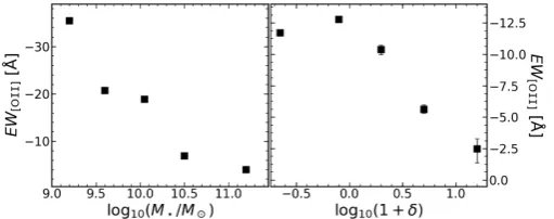
To quantify the properties of each line we have performed a double Gaussian fitting to [OII] using Equation1. Results of the equivalent widths and fluxes of the [OII] doublet are summarized in TableC.1and Figure11. The qualitative remarks we made on the appearance of the spectral stacks are confirmed by our results after fitting each component.

We find a strong decrease in [OII] strength and line equiva-lent width with stellar mass (see Figure11) with a factor of∼10

between the lowest stellar mass bin (9.0 < log10(M?/M) <

9.4) and the highest stellar mass bin (log₁₀(M?/M) > 10.7) (similar to results by e.g.Darvish et al. 2015a;Khostovan et al. 2016). Performing the same analysis on the stacked spectra per local density bin, the [OII] line strength and equivalent width show broken relation with a "break" atlog10(1+δ) ∼0.0−0.5 that translates into a steeper relation at higher densities.

5. Discussion

The survey that we present in this paper is able to select galax-ies through their continuum emission and absorption features down tolog₁₀(M?/M) ∼ 10and able to detect [OII] down to ∼5×10−18_{erg s}−1_cm−2_{. Since our sample is based on accurate} measurements of redshifts, it is natural that it selects galaxies at lower stellar masses only if they have clear emission lines char-acteristic of star-forming galaxies. This means that our results on global trends with stellar mass below our completeness limit is biased against low star formation and passive galaxies (see e.g. Figure4). This fact alone is able to explain an apparent lack of trends in star formation related quantities (SFR and L[OII])

at stellar masses belowlog₁₀(M?/M) =10, where we see no dependence whatsoever on local overdensity. In summary, our results for the lowest stellar mass bins (less than1010M) are likely based only on the star-forming population.

Fig. 10.Resulting spectral stacks (normalized by the flux at4150Å< λ <4350Å) around the [OII] doublet in bins of stellar mass (left) and in bins of local density (right). This figure shows the comparison between different stacks (for individual inspection we refer to FigureC.1). We see a strong dependence of the [OII] strength on the stellar mass with higher stellar mass galaxies having weaker [OII] emission, as expected since most quenched galaxies are found at higher stellar masses and should have little to no emission. We also find a dependence of the [OII] strength on the local density with high density regions having galaxies with weaker [OII] emission, again with massive quiescent galaxies dominating at higher densities likely the cause of this effect.

Fig. 11.Line equivalent width for the spectral lines in [OII] as a function of the stellar mass range (left) and of the local density range (right) for the stacked spectra. We apply no dust correction to the stacked derived values since we assume spatial coincidence between the continuum and line emitting regions, and they are affected by dust in a similar manner.

between stellar mass driven and density driven mechanisms (e.g. Peng et al. 2010;Kovaˇc et al. 2014;Darvish et al. 2016). We at-tempt to address these issues by computing average quantities in different environments as a function of stellar mass (or at differ-ent stellar masses as a function of environmdiffer-ent).

Considering our results on galaxies with stellar masses above our completeness limit, we find small influence of environment on galaxy SFRs (from SED fitting) and L[OII]. In higher

den-sity regions galaxies are typically less star-forming (Figure 8, except at the highest stellar masses (log10(M?/M) > 11) but with comparable [OII] emission. This can be easily explained by the increase of the fraction of quenched galaxies in higher density regions. These trends support the scenario where envi-ronment plays a role in increasing the quiescent fraction of in-termediate stellar mass galaxies at these redshifts (z ≈ 0.84). This fits well in the scenario where galaxies already have their star formation suppressed due to environmental effects as early as 7 billion years ago. At higher stellar masses, we see no

dif-ferences in the average SFR and quiescent fractions, hinting that mass quenching should be effective enough to halt star forma-tion even in low density regions (see e.g Peng et al. 2010) al-though it is not clear that environmental and stellar mass quench-ing are fully separable (see e.g.Lee et al. 2015;Darvish et al. 2016;Kawinwanichakij et al. 2017). This differential effect with stellar mass is a potential indicator that environment acts as a catalyst for star formation quenching in the sense that we are more likely to see galaxies quench at lower stellar masses if they reside in high density environments. We stress that for

10 < log₁₀(M?/M) < 10.25 we find no differences in the

median SFRs between low- and high-density regions and that is likely caused by a lack of quiescent galaxies close to our com-pleteness limit that drives up the median value of the SFR for that bin. Since we see a rise in the quiescent fraction towards high-density regions on the lowest stellar mass bin we probe (see Fig-ure9and also AppendixA), it is plausible that this is the reason for the observed results in this stellar mass bin.

5.1. Halting of star formation in the outskirts of clusters

Overall we find that the average SFR is lower in high-density regions, confirming what was reported by Sobral et al.(2011) when studying Hαemitters on the same structure. We report one order of magnitude difference in the average SFR from the low-est to the highlow-est density region (∼ 10 to∼ 1 Myr−1_{). This} trend with environment gives strength to the argument of envi-ronmentally driven quenching occurring within our superstruc-ture. These signs of environmental quenching of star formation (also seen in e.g.Patel et al. 2009; Sobral et al. 2011;Muzzin et al. 2012;Santos et al. 2013) are distinct from what one struc-tures that show a flat or reverse SFR-density relation (e.g.Elbaz et al. 2007;Ideue et al. 2009;Tran et al. 2010;Santos et al. 2014). One interesting result is the "break" that we find on the re-lation between [OII] line equivalent width and local overden-sity that occurs at intermediate densities (log10(δ) ∼ 0.0−0.5, see Fig.11and also e.g. Darvish et al. 2016). We hypothesize that this corresponds to a typical density where environment quenching mechanisms are the most effective. The transition atlog₁₀(δ) ∼ 0.0−0.5 is consistent with regions of filament-like densities (see transition from filament dominated to clus-ter dominated galaxies in Figure 6). This result is compatible with intermediate density regions likely being the place of en-hanced chances for galaxy encounters, promoting galaxy ha-rassment related quenching mechanisms (e.g.Moss 2006;Perez et al. 2009;Li et al. 2009;Tonnesen & Cen 2012;Darvish et al. 2014;Malavasi et al. 2017). It might also be caused by strong cluster-cluster interactions that are found to enhance star forma-tion as well (e.g.Stroe et al. 2014,2015). To further reinforce the existence of such "break", we find that the fraction of quenched galaxies at intermediate stellar masses (10<log₁₀(M?/M)< 10.75) increases by a factor of 2 at the same transition density, being roughly constant below and above. Galaxies at higher stel-lar masses are likely already quenched due to their own mass (see e.gPeng et al. 2010) and they are likely not much affected by the environment they are in.

6. Conclusions

We have presented in this paper an overview of the VIS3COS survey, which targets a superstructure at z ∼ 0.84 with VI-MOS/VLT high resolution spectra. We report on trends with en-vironment and stellar mass of the SFR and [OII] luminosity. Our main findings are summarized as follows:

– Above our stellar mass completeness limit (1010M), galax-ies in higher density regions have lower star formation rates at intermediate masses (10 < log₁₀(M?/M) < 10.75). At the highest masses (above1010.75_M

), the star formation

ac-tivity is similar in low- and high-density environments in-dicating that mass quenching is probably dominant at high stellar masses.

– We find that the fraction of quenched galaxies (fQ) in-creases from∼10% to∼40−60% with increasing galaxy overdensity, but only for intermediate stellar mass galaxies (10 < log₁₀(M?/M) < 10.75). The most massive galax-ies in our sample (above1010.75M) have a similar value of

fQ ∼30−40% at all densities.

– We find a break in [OII] strength and equivalent width in the stacked spectra in filament-like regions (log₁₀(δ) ∼0.0−

0.5). We hypothesize that at these densities quenching mech-anisms due to environment play an important role. This is

consistent with the increase in the quenched galaxy fraction that we find for intermediate stellar mass galaxies.

In summary, the results of this paper shed some light on the properties of galaxies in and around a superstructure on the COSMOS field. In this paper we have focused on the overall properties of the sample in our survey and the general trends that we find on galaxy properties with respect to environment. More detailed studies focusing on the individual star formation activity of galaxies, galaxy morphology, and electron density estimates will be discussed in forthcoming papers.

Acknowledgements

We thank the anonymous referee for making valuable sugges-tions that helped to improve this paper. This work was sup-ported by Fundação para a Ciência e a Tecnologia (FCT) through the research grant UID/FIS/04434/2013. APA, PhD::SPACE fellow, acknowledges support from the FCT through the fel-lowship PD/BD/52706/2014. DS acknowledges financial sup-port from the Netherlands Organisation for Scientific research (NWO) through a Veni fellowship and from Lancaster University through an Early Career Internal Grant A100679. BD acknowl-edges financial support from NASA through the Astrophysics Data Analysis Program (ADAP), grant number NNX12AE20G, and the National Science Foundation, grant number 1716907. PNB is grateful for support from STFC via grant ST/M001229/1. This work was only possible by the use of the following PYTHON packages: NumPy & SciPy (Walt et al. 2011; Jones et al. 2001), Matplotlib (Hunter 2007), and Astropy (Astropy Collaboration et al. 2013).

References

Aragón-Calvo, M. A., van de Weygaert, R., & Jones, B. J. T. 2010, MNRAS, 408, 2163

Astropy Collaboration, Robitaille, T. P., Tollerud, E. J., et al. 2013, A&A, 558, A33

Baldry, I. K., Balogh, M. L., Bower, R. G., et al. 2006, MNRAS, 373, 469 Balogh, M., Eke, V., Miller, C., et al. 2004, MNRAS, 348, 1355

Balogh, M. L., Couch, W. J., Smail, I., Bower, R. G., & Glazebrook, K. 2002, MNRAS, 335, 10

Balogh, M. L., McGee, S. L., Mok, A., et al. 2014, MNRAS, 443, 2679 Bamford, S. P., Nichol, R. C., Baldry, I. K., et al. 2009, MNRAS, 393, 1324 Beers, T. C., Flynn, K., & Gebhardt, K. 1990, AJ, 100, 32

Bekki, K. 2009, MNRAS, 399, 2221 Best, P. N. 2004, MNRAS, 351, 70

Boselli, A., Cortese, L., Boquien, M., et al. 2014, A&A, 564, A67 Brown, T., Catinella, B., Cortese, L., et al. 2017, MNRAS, 466, 1275 Bruzual, G. & Charlot, S. 2003, MNRAS, 344, 1000

Burgarella, D., Buat, V., Gruppioni, C., et al. 2013, A&A, 554, A70

Canto, J., Meaburn, J., Theokas, A. C., & Elliott, K. H. 1980, MNRAS, 193, 911 Carollo, C. M., Bschorr, T. J., Renzini, A., et al. 2013, ApJ, 773, 112

Chabrier, G. 2003, ApJ, 586, L133 Charlot, S. & Fall, S. M. 2000, ApJ, 539, 718

Cohen, S. A., Hickox, R. C., Wegner, G. A., Einasto, M., & Vennik, J. 2017, ApJ, 835, 56

Cooper, M. C., Newman, J. A., Weiner, B. J., et al. 2008, MNRAS, 383, 1058 Cortese, L., Davies, J. I., Pohlen, M., et al. 2010, A&A, 518, L49

Crain, R. A., Schaye, J., Bower, R. G., et al. 2015, MNRAS, 450, 1937 Cucciati, O., Davidzon, I., Bolzonella, M., et al. 2017, A&A, 602, A15 Cucciati, O., Iovino, A., Kovaˇc, K., et al. 2010a, A&A, 524, A2 Cucciati, O., Marinoni, C., Iovino, A., et al. 2010b, A&A, 520, A42 Cucciati, O., Zamorani, G., Lemaux, B. C., et al. 2014, A&A, 570, A16 da Cunha, E., Charlot, S., & Elbaz, D. 2008, MNRAS, 388, 1595 Darvish, B., Mobasher, B., Martin, D. C., et al. 2017, ApJ, 837, 16 Darvish, B., Mobasher, B., Sobral, D., et al. 2015a, ApJ, 814, 84 Darvish, B., Mobasher, B., Sobral, D., et al. 2016, ApJ, 825, 113

Darvish, B., Mobasher, B., Sobral, D., Scoville, N., & Aragon-Calvo, M. 2015b, ApJ, 805, 121

Draine, B. T. 2004, in The Cold Universe, Saas-Fee Advanced Course 32, Springer-Verlag, 308 pages, 129 figures, Lecture Notes 2002 of the Swiss Society for Astronomy and Astrophysics (SSAA), Springer, 2004. Edited by A.W. Blain, F. Combes, B.T. Draine, D. Pfenniger and Y. Revaz, ISBN 354040838x, p. 213, ed. A. W. Blain, F. Combes, B. T. Draine, D. Pfenniger, & Y. Revaz, 213

Dressler, A. 1980, ApJ, 236, 351 Dressler, A. 1984, ARA&A, 22, 185

Ehlert, S., von der Linden, A., Allen, S. W., et al. 2014, MNRAS, 437, 1942 Elbaz, D., Daddi, E., Le Borgne, D., et al. 2007, A&A, 468, 33

Ellison, S. L., Patton, D. R., Simard, L., & McConnachie, A. W. 2008, AJ, 135, 1877

Finoguenov, A., Guzzo, L., Hasinger, G., et al. 2007, ApJS, 172, 182 Fumagalli, M., Labbé, I., Patel, S. G., et al. 2014, ApJ, 796, 35 Gallazzi, A., Bell, E. F., Wolf, C., et al. 2009, ApJ, 690, 1883

Genel, S., Vogelsberger, M., Springel, V., et al. 2014, MNRAS, 445, 175 Giovanelli, R. & Haynes, M. P. 1985, ApJ, 292, 404

Gómez, P. L., Nichol, R. C., Miller, C. J., et al. 2003, ApJ, 584, 210 Hayashi, M., Kodama, T., Koyama, Y., et al. 2014, MNRAS, 439, 2571 Henriques, B. M. B., White, S. D. M., Thomas, P. A., et al. 2015, MNRAS, 451,

2663

Hogg, D. W., Blanton, M. R., Brinchmann, J., et al. 2004, ApJ, 601, L29 Hunter, J. D. 2007, Computing In Science & Engineering, 9, 90 Ideue, Y., Nagao, T., Taniguchi, Y., et al. 2009, ApJ, 700, 971 Ilbert, O., Capak, P., Salvato, M., et al. 2009, ApJ, 690, 1236 Ilbert, O., McCracken, H. J., Le Fèvre, O., et al. 2013, A&A, 556, A55 Ilbert, O., Salvato, M., Le Floc’h, E., et al. 2010, ApJ, 709, 644 Iovino, A., Cucciati, O., Scodeggio, M., et al. 2010, A&A, 509, A40 Iovino, A., Petropoulou, V., Scodeggio, M., et al. 2016, A&A, 592, A78 Jones, E., Oliphant, T., Peterson, P., et al. 2001, SciPy: Open source scientific

tools for Python, [Online; accessed 2016-03-23]

Kaasinen, M., Bian, F., Groves, B., Kewley, L. J., & Gupta, A. 2017, MNRAS, 465, 3220

Karim, A., Schinnerer, E., Martínez-Sansigre, A., et al. 2011, ApJ, 730, 61 Kauffmann, G., White, S. D. M., Heckman, T. M., et al. 2004, MNRAS, 353,

713

Kawinwanichakij, L., Papovich, C., Quadri, R. F., et al. 2017, ApJ, 847, 134 Kennicutt, Jr., R. C. 1998, ARA&A, 36, 189

Kewley, L. J., Geller, M. J., & Barton, E. J. 2006, AJ, 131, 2004 Kewley, L. J., Geller, M. J., & Jansen, R. A. 2004, AJ, 127, 2002

Khostovan, A. A., Sobral, D., Mobasher, B., et al. 2015, MNRAS, 452, 3948 Khostovan, A. A., Sobral, D., Mobasher, B., et al. 2016, MNRAS, 463, 2363 Kocevski, D. D., Lemaux, B. C., Lubin, L. M., et al. 2011, ApJ, 737, L38 Kodama, T., Balogh, M. L., Smail, I., Bower, R. G., & Nakata, F. 2004, MNRAS,

354, 1103

Koekemoer, A. M., Aussel, H., Calzetti, D., et al. 2007, ApJS, 172, 196 Kovaˇc, K., Lilly, S. J., Knobel, C., et al. 2014, MNRAS, 438, 717 Koyama, S., Koyama, Y., Yamashita, T., et al. 2017, ApJ, 847, 137 Koyama, Y., Kodama, T., Tadaki, K.-i., et al. 2014, ApJ, 789, 18 Koyama, Y., Smail, I., Kurk, J., et al. 2013, MNRAS, 434, 423 Kulas, K. R., McLean, I. S., Shapley, A. E., et al. 2013, ApJ, 774, 130 Laigle, C., McCracken, H. J., Ilbert, O., et al. 2016, ApJS, 224, 24

Le Fèvre, O., Saisse, M., Mancini, D., et al. 2003, in Proc. SPIE, Vol. 4841, Instrument Design and Performance for Optical/Infrared Ground-based Tele-scopes, ed. M. Iye & A. F. M. Moorwood, 1670–1681

Lee, S.-K., Im, M., Kim, J.-W., et al. 2015, ApJ, 810, 90

Lemaux, B. C., Cucciati, O., Tasca, L. A. M., et al. 2014, A&A, 572, A41 Lewis, I., Balogh, M., De Propris, R., et al. 2002, MNRAS, 334, 673 Li, I. H., Glazebrook, K., Gilbank, D., et al. 2011, MNRAS, 411, 1869 Li, I. H., Yee, H. K. C., & Ellingson, E. 2009, ApJ, 698, 83

Lilly, S. J., Le Fevre, O., Hammer, F., & Crampton, D. 1996, ApJ, 460, L1 Lilly, S. J., Le Fèvre, O., Renzini, A., et al. 2007, ApJS, 172, 70

Lubin, L. M., Gal, R. R., Lemaux, B. C., Kocevski, D. D., & Squires, G. K. 2009, AJ, 137, 4867

Madau, P. & Dickinson, M. 2014, ARA&A, 52, 415

Malavasi, N., Arnouts, S., Vibert, D., et al. 2017, MNRAS, 465, 3817 Malavasi, N., Pozzetti, L., Cucciati, O., Bardelli, S., & Cimatti, A. 2016, A&A,

585, A116

Masters, D. & Capak, P. 2011, PASP, 123, 638 Mihos, J. C. & Hernquist, L. 1996, ApJ, 464, 641

Mok, A., Balogh, M. L., McGee, S. L., et al. 2013, MNRAS, 431, 1090 Mok, A., Wilson, C. D., Golding, J., et al. 2016, MNRAS, 456, 4384 Moss, C. 2006, MNRAS, 373, 167

Mulroy, S. L., McGee, S. L., Gillman, S., et al. 2017, MNRAS, 472, 3246 Muzzin, A., Marchesini, D., Stefanon, M., et al. 2013, ApJS, 206, 8 Muzzin, A., Wilson, G., Yee, H. K. C., et al. 2012, ApJ, 746, 188

Nakata, F., Bower, R. G., Balogh, M. L., & Wilman, D. J. 2005, MNRAS, 357, 679

Noeske, K. G., Weiner, B. J., Faber, S. M., et al. 2007, ApJ, 660, L43 Oemler, Jr., A. 1974, ApJ, 194, 1

Oh, S., Mulchaey, J. S., Woo, J.-H., et al. 2014, ApJ, 790, 43

Owers, M. S., Couch, W. J., Nulsen, P. E. J., & Randall, S. W. 2012, ApJ, 750, L23

Patel, S. G., Holden, B. P., Kelson, D. D., Illingworth, G. D., & Franx, M. 2009, ApJ, 705, L67

Peng, Y.-j., Lilly, S. J., Kovaˇc, K., et al. 2010, ApJ, 721, 193 Pentericci, L., Castellano, M., Menci, N., et al. 2013, A&A, 552, A111 Perez, J., Tissera, P., Padilla, N., Alonso, M. S., & Lambas, D. G. 2009, MNRAS,

399, 1157

Poggianti, B. M., Aragón-Salamanca, A., Zaritsky, D., et al. 2009, ApJ, 693, 112 Poggianti, B. M., von der Linden, A., De Lucia, G., et al. 2006, ApJ, 642, 188 Pradhan, A. K., Montenegro, M., Nahar, S. N., & Eissner, W. 2006, MNRAS,

366, L6

Rodríguez del Pino, B., Aragón-Salamanca, A., Chies-Santos, A. L., et al. 2017, MNRAS, 467, 4200

Roediger, E., Brüggen, M., Owers, M. S., Ebeling, H., & Sun, M. 2014, MNRAS, 443, L114

Salpeter, E. E. 1955, ApJ, 121, 161

Sanders, R. L., Shapley, A. E., Kriek, M., et al. 2016, ApJ, 816, 23 Santos, J. S., Altieri, B., Popesso, P., et al. 2013, MNRAS, 433, 1287 Santos, J. S., Altieri, B., Tanaka, M., et al. 2014, MNRAS, 438, 2565 Schaye, J., Crain, R. A., Bower, R. G., et al. 2015, MNRAS, 446, 521 Scoville, N., Arnouts, S., Aussel, H., et al. 2013, ApJS, 206, 3 Seaton, M. J. & Osterbrock, D. E. 1957, ApJ, 125, 66

Serra, P., Oosterloo, T., Morganti, R., et al. 2012, MNRAS, 422, 1835 Shimakawa, R., Kodama, T., Hayashi, M., et al. 2018, MNRAS, 473, 1977 Shimakawa, R., Kodama, T., Tadaki, K.-i., et al. 2015, MNRAS, 448, 666 Sobral, D., Best, P. N., Geach, J. E., et al. 2009, MNRAS, 398, 75 Sobral, D., Best, P. N., Smail, I., et al. 2011, MNRAS, 411, 675 Sobral, D., Smail, I., Best, P. N., et al. 2013, MNRAS, 428, 1128 Sobral, D., Stroe, A., Dawson, W. A., et al. 2015, MNRAS, 450, 630 Sobral, D., Stroe, A., Koyama, Y., et al. 2016, MNRAS, 458, 3443 Stroe, A. & Sobral, D. 2015, MNRAS, 453, 242

Stroe, A., Sobral, D., Dawson, W., et al. 2015, MNRAS, 450, 646 Stroe, A., Sobral, D., Paulino-Afonso, A., et al. 2017, MNRAS, 465, 2916 Stroe, A., Sobral, D., Röttgering, H. J. A., & van Weeren, R. J. 2014, MNRAS,

438, 1377

Tadaki, K.-i., Kodama, T., Ota, K., et al. 2012, MNRAS, 423, 2617 Tonnesen, S. & Cen, R. 2012, MNRAS, 425, 2313

Tran, K.-V. H., Papovich, C., Saintonge, A., et al. 2010, ApJ, 719, L126 Treu, T., Ellis, R. S., Kneib, J.-P., et al. 2003, ApJ, 591, 53

van der Wel, A., Noeske, K., Bezanson, R., et al. 2016, ApJS, 223, 29 Vogelsberger, M., Genel, S., Springel, V., et al. 2014, Nature, 509, 177 Walt, S. v. d., Colbert, S. C., & Varoquaux, G. 2011, Computing in Science &

Engineering, 13, 22

Whitaker, K. E., van Dokkum, P. G., Brammer, G., & Franx, M. 2012, ApJ, 754, L29

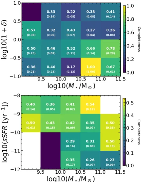
Fig. A.1.Spectroscopic sample completeness as a function of stellar mass and local overdensity (top) and specific star formation rate (bot-tom). In each panel we indicate in white numbers the completeness for each bin (Poisson errors shown in parenthesis). Bins with no targets are shown in white.

Appendix A: Sample Completeness

We estimate the sample completeness of our spectroscopic ob-servations by comparing the number of sources for which we successfully measured a redshift with the number of possible targets in the parent catalogue (given our selection described in Section2.2). We present our results in FigureA.1. We will dis-cuss the completeness effects in more detail in a forthcoming paper.

We confirm that we are under-sampling denser regions when compared to the lowest density regions, which is expected given the spatial constraints on the positioning of the slits in the VI-MOS masks does not allow to target densely populated areas. In terms of star formation activity we find that our typical complete-ness is lower for quiescent galaxies (∼30%) when compared to star-forming ones (∼ 40%). When taken together we find that we are most likely missing quiescent galaxies in high density re-gions, but that the difference between the two populations is not dramatic in terms of completeness and our derived completeness corrections can tackle this without problems. Therefore we are providing a fair representation of the galaxy population in the regions we are targeting.

Appendix B: Catalogue of superstructure

members

We release with this paper the VIS3COS catalogue of all targets in and around the superstructure at z ∼ 1 with spectroscopic redshifts, along with some of their measured properties: SFR,

overdensity, stellar mass. We present the first 10 entries of the full catalogue in TableB.1.

Appendix C: Individual Stacks

Table B.1.First 10 galaxies in our sample. The first column is our catalogue ID. The second and third two columns show the object coordinates fromIlbert et al.(2009). The fourth column is our measured spectroscopic redshift. The fifth column is theK-band magnitude fromIlbert et al.

(2009). The sixth and seventh columns are the stellar masses and SFRs derived withMAGPHYS. The last column is the local overdensity from

Darvish et al.(2015b,2017).

ID RA DEC zspec KAB log10(M?) log10(SF R) log10(1+δ)

(J2000) (J2000) (M) (Myr−1)

VIS3COS-1 150.510640 2.035566 0.8998 20.6 10.6 0.9 -0.26

VIS3COS-2 150.521776 2.040788 0.8707 21.0 10.4 0.1 0.15

VIS3COS-3 150.547778 2.044605 0.8714 20.5 11.0 0.5 0.39

VIS3COS-4 150.543696 2.047819 0.8080 21.9 9.2 0.6 -0.68

VIS3COS-6 150.590194 2.051661 0.8419 20.0 10.6 1.1 0.11

VIS3COS-7 150.573302 2.053824 0.8722 21.5 10.4 1.3 -0.19

VIS3COS-8 150.520207 2.057174 0.8970 21.1 10.1 1.1 0.28

VIS3COS-10 150.569219 2.062002 0.6980 19.7 11.2 1.5 -0.54

VIS3COS-12 150.575212 2.068181 0.8724 99.0 10.5 -0.7 -0.09

VIS3COS-13 150.538943 2.070524 0.8930 20.5 10.8 0.2 0.14

VIS3COS-15 150.604440 2.074035 0.8555 21.9 9.6 0.3 0.03

Table C.1.Summary of [OII] properties from the stacked spectra. Equivalent widths (EW) are in units of Å. The third column shows the doublet ratioR=[OII]λ3729/λ3726.

Range EW([OII]) R

9.0<log₁₀(M?/M)<9.4 −35.4+₋0₀._.4₄ 1.46+₋0₀._.07₀₇ 9.4<log₁₀(M?/M)<9.8 −20.7+₋0₀._.2₂ 1.45+₋0₀._.06₀₆ 9.8<log₁₀(M?/M)<10.3 −18.9+₋0₀._.2₂ 1.43+₋0₀._.06₀₆ 10.3<log10(M?/M)<10.7 −6.9+₋0₀._.3₂ 1.16+₋0₀._.10₁₀ 10.7<log₁₀(M?/M)<11.7 −4.0+₋0₀._.2₂ 1.09+₋0₀._.08₀₈

−1.0<log10(1+δ)<−0.3 −11.7+−00..22 1.59+ 0.07

−0.07 −0.3<log₁₀(1+δ)<0.1 −12.8+0.2

−0.2 1.26+ 0.05

−0.05

0.1<log₁₀(1+δ)<0.5 −10.4+0.4

−0.4 1.23+−00..0808

0.5<log10(1+δ)<0.9 −5.6+−00..33 1.15+ 0.09

−0.09

0.9<log10(1+δ)<1.5 −2.5+−10..18 1.31+ 0.47

Fig. C.1.Resulting spectral stacks (solid black line) in bins of stellar mass (high to low stellar mass from top to bottom) around the [OII] dou-blet. We show in green the best fit doublet model with each component shown as blue and red dashed lines. The shaded grey area represents the typical error on the fit of the spectra at each wavelength computed from the 16th and 84th percentiles of 10000 realizations of perturbing the spectra by its error. In each panel we show the derived ratio between the two doublet components.