warwick.ac.uk/lib-publications
Original citation:
Yazdani, Danial , Nguyen, Trung Thanh and Branke, Jürgen (2018) Robust optimization over
time by learning problem space characteristics. IEEE Transactions on Evolutionary
Computation.
doi:
10.1109/TEVC.2018.2843566
Permanent WRAP URL:
http://wrap.warwick.ac.uk/102784
Copyright and reuse:
The Warwick Research Archive Portal (WRAP) makes this work by researchers of the
University of Warwick available open access under the following conditions. Copyright ©
and all moral rights to the version of the paper presented here belong to the individual
author(s) and/or other copyright owners. To the extent reasonable and practicable the
material made available in WRAP has been checked for eligibility before being made
available.
Copies of full items can be used for personal research or study, educational, or not-for profit
purposes without prior permission or charge. Provided that the authors, title and full
bibliographic details are credited, a hyperlink and/or URL is given for the original metadata
page and the content is not changed in any way.
Publisher’s statement:
“© 2018 IEEE. Personal use of this material is permitted. Permission from IEEE must be
obtained for all other uses, in any current or future media, including reprinting
/republishing this material for advertising or promotional purposes, creating new collective
works, for resale or redistribution to servers or lists, or reuse of any copyrighted component
of this work in other works.”
A note on versions:
The version presented here may differ from the published version or, version of record, if
you wish to cite this item you are advised to consult the publisher’s version. Please see the
‘permanent WRAP URL’ above for details on accessing the published version and note that
access may require a subscription.
Robust optimization over time by learning problem
space characteristics
Danial Yazdani, Trung Thanh Nguyen, and J¨urgen Branke
Abstract—Robust optimization over time is a new way to tackle dynamic optimization problems where the goal is to find solutions that remain acceptable over an extended period of time. The state-of-the-art methods in this domain try to identify robust solutions based on their future predicted fitness values. However, predicting future fitness values is difficult and error prone. In this paper, we propose a new framework based on a multi-population method in which sub-populations are responsible for tracking peaks and also gathering characteristic information about them. When the quality of the current robust solution falls below the acceptance threshold, the algorithm chooses the next robust solution based on the collected information. We propose four different strategies to select the next solution. The experimental results on benchmark problems show that our newly proposed methods perform significantly better than existing algorithms.
Index Terms—Dynamic optimization problems, Robust opti-mization over time, Tracking moving optima, Particle Swarm Optimization
I. INTRODUCTION
M
ANY real-world optimization problems are dynamic and changing over time. Most previous studies in this domain focus on tracking the moving optimum (TMO) [1]. However, this is not practical in many real-world cases since changing solutions may be very costly, and changing the so-lution frequently is not desirable. For example, in scheduling, changing the schedule may have significant impact on sup-pliers and customers, or, in the design of telephone networks, sending out engineers to change the physical infrastructure can be very expensive. In taking-off/landing scheduling problem, it is desirable to keep the current implemented solution/schedule after an environmental change [2], [3] to avoid unfavorable disruptions in airport operations. To address such a problem, [4] proposed a new approach for solving dynamic optimization problems (DOP): finding solutions that are robust over the course of time. A robust solution is one that is not necessarily the best in the current environment, but that remains acceptableThis work was supported in part by a Dean’s Scholarship by Faculty of Engineering and Technology, LJMU, a Newton Institutional Links grant no. 172734213, funded by the UK BEIS and delivered by the British Council, and a NRCP grant no. NRCP1617-6-125 delivered by Royal Academy of Engineering.
D. Yazdani is with the Liverpool Logistics, Offshore and Marine Re-search Institute, Department of Maritime and Mechanical Engineering, Liverpool John Moores University, Liverpool L3 3AF, United Kingdom (Email:[email protected], [email protected]).
T. T. Nguyen is with the Department of Maritime and Mechanical Engineer-ing, Liverpool John Moores University, Liverpool L3 3AF, United Kingdom (Email:[email protected]).
J. Branke is with the Operational Research and Management Sciences Group in Warwick Business school, University of Warwick, Coventry CV4 7AL, United Kingdom (Email:[email protected]).
over several environments. A found robust solution can be utilized until its quality degrades to an unacceptable level.
In case the current robust solution becomes unsatisfactory, a new robust solution must be chosen. The process of finding a sequence of robust solutions is referred to as robust opti-mization over time (ROOT) [4], [5]. A DOP can be defined as:
F(x) =f(x, θ(t)), (1) wheref is the objective function,xis a design vector, θ(t) is environmental parameters which change over time andtis the time index with t∈[0, T] whereT is the problem life cycle or number of environments. In this paper, like most previous studies in the DOP domain, we investigate DOPs with θ(t)
that changes discretely. In this type of DOP, the environmental parameters change over time with stationary periods between changes. As a result, for a DOP withTenvironmental changes, we have a sequence of T static environments that can be described as:
F(x) =hf(x, θ(1)), f(x, θ(2)), . . . , f(x, θ(T))i, (2) where θ(i) represents the environmental parameters in the
ith environment. For ROOT, the main goal is to minimize the number of times the chosen solution has to be changed because its performance drops below an acceptable level, or to maximize the average number of environments that a robust solution remains acceptable. Thus, the best case is that the first robust solution remains acceptable for all of the T environments and the worst case is that the number of robust solutions is equal to the number of environments (none of the solutions remained acceptable after even a single environmental change).
The rest of this paper is structured as follows. In Section II, related works are reviewed. In Section III, the proposed framework is presented. Section IV explains the experimental setup including benchmarks, performance indicators, compar-ison algorithms and parameter settings of all tested methods. Experimental results, analyses and comparisons with previous works are reported in Section V. In the final section, we summarize the main findings and suggest directions for future work.
II. RELATED WORKS
The proposed framework uses population or multi-swarm methods for ROOT. Therefore, in this section, we provide a more detailed literature review on ROOT as the main topic of this paper, as well as a brief review on multi-population/multi-swarm methods.
A. Robust optimization over time
In [4], ROOT was proposed as a new perspective on DOPs. A new framework for ROOT was proposed in [6] with the algorithm searching for robust solutions by means of local fitness approximation and prediction. This method consists of a population-based optimization algorithm, a fitness approximator (to estimate fitness at any point in the search space), a fitness predictor (to predict future fitness values) and a database. In [6], an adapted radial-basis-function network (RBFN) is the local approximator and an autoregressive (AR) is the predictor. A database was used for storing, in each iteration, all of the individuals’ positions alongside their fitness values and the associated time of storage. This database was then used for approximating fitness values of solutions in previous environments which in turn was used for training the predictor.
It is important to have sufficient samples across the search space in this database to maintain the accuracy of the ap-proximation. Since optimization algorithms quickly converge to the most promising region in the search space, there would be regions that they would not visit (such as regions with bad fitness) which still are necessary for having a good training data. On the one hand, in [6], the algorithm needs to have enough information to be able to predict any solution in the search space which is depended on the approximator. On the other hand, for having an appropriate approximation model, the training data needs to be properly distributed in the search space. For achieving this, in [6], authors generate half of the population using a specific hypercube design after each environmental change. Therefore, for each environment, the database can contain at least one solution from each hypercube. However, in larger environments such as ones with bigger search range and higher dimensions, the number of these hypercubes increases exponentially and becomes larger than the population size. As a result, the algorithm needs to evaluate a solution for each hypercube for adding to the database. These additional fitness evaluations become a challenge in larger problems.
To select a robust solution, [6] uses the sum of the solutions’ current fitness value, itspprevious fitness values (provided by
the approximator) and itsqfuture fitness values (provided by the predictor):
F(x) =
t+q
X
l=t−p
f(x, θ(l)), (3) whereF is the sum of fitness values ofxat timet. The perfor-mance of the proposed method in [6] depends on the accuracy of the approximation and prediction methods. In [6], a particle swarm optimization (PSO) [7] was used as the optimizer. In addition, several performance indicators were proposed, of which one of the most important ones is Eavg, the average error of the robust solution sequenceS= (r1,r2,· · ·,rk),
Eavg=
1 k
k
X
i=1
ei, (4)
where
ei=
1 ni
ti+ni−1
X
j=ti
opt
(j)−f(r i, θ(j))
, (5)
opt(j)is the optimum fitness value at thejthenvironment,riis theithrobust solution,niis number of environments for which
ri remained acceptable, andtiis the time thatriwas chosen. In other words,Eavg is the average error of robust solutions over all environments. Another performance indicator isρ, the robustness rate of the robust solution sequence,
ρ= 1− k−1
T−1, (6)
wherekis the number of robust solutions. In (6), a smallerk
causesρto increase and the ideal situation happens when the first robust solution can remain acceptable in all environments i.e.k= 1. In addition, a new condition for checking whether a robust solution may be kept in a new environment was introduced. According to this condition, given a user defined threshold δdrop, a robust solution ri may be kept in the jth environment if:
f(ri, θ(j))−opt(j)
opt(j)
≤δdrop. (7)
In [8], authors proposed two new robustness definitions and metrics, namely survival time and average fitness. The survival time is the maximum time interval starting from time
tduring which the fitness value of the robust solution remains acceptable:
Sx, θ(t), V=
0 iff(x, θ(t))< V
1 + max{l| ∀i∈ {t, . . . , t+l}:f
x, θ(i)≥V} otherwise
(8)
whereV is a user defined threshold. In (8), for each environ-ment,Sshows for how many environments the fitness value of the current solution has remained aboveV. Note the threshold
V in [8] is easier to use than δdrop in (7) from [6] which requires to know the optimum.
The robust solution is selected based on the predicted average fitness over a pre-defined time windowω as follows:
Ax, θ(t), ω= 1 ω
ω−1
X
i=0
When (8) and (9) are used as metrics, f(x, θ(i))for i > t is predicted fitness value of x in tth environment instead of its actual fitness value. In the experiments in [8], the authors assumed that the algorithm benefited from an ideal approx-imator so they used true previous fitness values instead of approximated fitness values. Consequently, the reported results in [8] were not subject to approximation errors. Additionally, a ROOT performance indicator was proposed in this paper based on (8) and (9) as follows:
P = 1 T
T
X
i=1
F(i), (10)
where P is performance of ROOT algorithm, F(i) is either
S in (8) or A in (9). In [9], two definitions of ROOT in [8] i.e. survival time and average fitness were analyzed. Also, two different benchmark problems were proposed.
In [10], a new two-layer multi-objective method was proposed to find robust solutions that can maximize both survival time and average fitness. In [11], another multi-objective method was proposed to minimize switching cost and maximize survival time. A PSO algorithm was used as the optimizer. Additionally, the algorithm used the acceptance threshold for robust solutions similar to [8]. Euclidean distance between two solutions was used as the switching cost, and three different performance indicators were used:
F= 1 T
T
X
i=1
Fi, (11)
R= 1 T
T
X
i=1
Ri, (12)
C= 1 T
T
X
i=1
Ci, (13)
where T is number of environments, Fi is fitness value of robust solutions,Riis robustness (calculated by (8)) andCiis switching cost inithenvironment. Switching cost is Euclidean distance between robust solutions in successive environments. All of the proposed methods in [6], [8], [9] and [11] used predicted future fitness values of solutions for selecting robust solutions. In [6], an RBFN was used for approximating previous fitness values of solutions and an AR was used for predicting future values. In [8], the authors removed the approximation part and used true fitness values in previous environments for training the AR in order to remove the negative effect of approximation errors on the performance of the algorithms. In [9], the authors used the same methods as in [6] for approximation and prediction to investigate the performance of the proposed algorithms in [6] and [8]. In [11], the authors assumed that algorithms benefited from an ideal predictor without any error, so in their experiments the true future fitness values were used instead of the predicted values. However, removing the approximator and predictor from algorithms that work based on future fitness values of solutions clearly is a substantial simplification and the
performance on a real-world problem where future fitness values are not available may be very different. Overall, for solving real-world problems, almost all the current ROOT methods [6], [8]–[10] and [11] need to use approximation and prediction methods based on time series [12].
B. Tracking Moving Optimum
Multi-population/multi-swarm methods are popular among researchers in the DOP domain [1], [13]. They consist of at least two sub-populations/swarms handling different tasks or separate regions in the problem space.
In [14], Self Organizing Scouts (SOS) was proposed which utilized a big sub-population for global search and a number of small sub-populations for tracking changes of identified peaks. This strategy has also been proposed with other meta-heuristics such as PSO [15]–[18] and artificial fish swarm optimization [19]–[21].
In [22], a speciation method was used to split the population into sub-populations. In [23], a regression-based approach (RSPSO) was presented to enhance the convergence rate using speciation-based methods. Every subpopulation was confined to a hypersphere around the best solution.
In [24], a method based on clustering was proposed for developing sub-populations, which was simplified and further improved in [25]. In [26], a method called MEPSO was proposed in which the population was divided into two parts. The first part was responsible for exploitation and the second one for exploration. Gaussian local search and differential mutation were used to improve diversity in the environment.
In [27], two multi-population methods, called MQSO and MCPSO, were proposed. In MQSO, quantum particles appear at random positions, uniformly distributed around the swarm’s global best. In MCPSO, some or all of the particles in each swarm have a ‘charge’, and charged particles repel each other, leading to larger diversity. The population size is equal for every sub-swarm, and the number of sub-swarms is fixed and pre-determined. An anti-convergence method ensures contin-ued search for possible better peaks. In addition, a mechanism called exclusion is used to avoid several swarms converging to the same peak.
A version of MQSO with an adaptive number of sub-populations, called AMQSO, was proposed in [28]. AMQSO starts with one sub-population and a new sub-population is created if all previous sub-populations have converged. This method has significantly improved the performance.
Li et al [29] proposed a method to adapt the number of populations based on statistical data on how many popula-tions have found new peaks. If this number is large, more populations will be introduced and vice versa. Additionally, a new heuristic clustering, a population hibernation scheme, a population exclusion scheme, a peak hiding method and two movement methods (to track peaks and avoid stagnation) were proposed.
An exclusion mechanism re-initializes the finder swarm if it converges to a peak that already has a tracker swarm on it. In addition, a mechanism to schedule tracker swarms called sleeping-awakening was proposed. It allocates more computational power to more promising swarms. Furthermore, a new method for re-diversification of tracker swarms (after a change) was proposed. The method re-initializes all parti-cles randomly around Gbest [7] and their velocity vector is randomly set based on the peak’s shift severity. In [31], a hybrid method based on FTmPSO was proposed for DOPs with previous-solution displacement restriction (PSDR).
III. THEPROPOSEDFRAMEWORK
The literature review above shows that almost all current methods on ROOT need to use approximation and prediction methods based on time series [12]. The accuracy of this approach depends on the amount of data available, i.e. past and current fitness values covering the representative regions of the search space. In problems with a large number of dimensions and/or large search space and/or high change frequency, a very large amount of data is required to obtain an accurate approximation. This may be impossible to achieve. In this section, we propose a new framework for ROOT that does not rely on predicted future values of solutions. Consequently, the proposed framework does not require complicated approx-imation and prediction methods for predicting solution fitness values. Instead, a multi-population algorithm is responsible to find peaks, track them after environmental changes and gather information about their behavior. This information will be used to predict the future behavior of peaks. When the current solution becomes unacceptable, the next robust solution will be selected by a decision rule based on information collected by sub-populations such as shift severity or height severity. In this paper, we propose four such decision rules.
A. The multi-population/multi-swarm method
In this section, we describe the necessary characteristics of multi-population (or multi-swarm) methods that can be used inside the proposed ROOT framework. We assume a multi-population algorithm would continuously try to identify new peaks and track them after an environmental change. Knowledge about the problem such as number of peaks and their shift severities should not be necessary. Additionally, the algorithm should be able to adapt the number of populations as needed. For example, the proposed multi-population methods in [28], [30] have such characteristics.
The other requirement is preventing overcrowding, i.e., each peak should be covered by at most one sub-population. Typically, algorithms use an exclusion mechanism [27] for this purpose. If the distance between the best found positions of two populations drops below some exclusion radiusrexcl, the population with the worse best found position is re-initialized. A good formula for calculating rexcl without a need to know the number of peaks was proposed in [28] as follows:
rexcl=exclfactor×
SR
T SND1
, (14)
where exclfactor is a positive constant less than 1, SR is the search domain, T SN is the current number of sub-populations and D is the number of dimensions. It is worth mentioning that the original formula in [27] used number of peaks instead of T SN which usually is unknown in real-world problems. This was changed toT SN in [28]. Note that, in the proposed framework, each sub-population separately records some information about its covered peak. Therefore, the exclusion mechanism for the proposed framework should allow such a record to be transferred from one population to another before the population is re-initialized. If the surviving population is younger (according to the environment number that it was created), then before the algorithm re-initializes the older one, its database will be transferred to the surviving one. Another characteristic that a compatible multi-population method should have is being able to track peaks. Therefore, the populations that are responsible to cover and track peaks need to be able to deal with diversity loss [1]. In [1], methods that deal with diversity were grouped into two categories: methods that maintain diversity during the search and the methods that introduce diversity when changes occur. Additionally, to track peaks, populations need to deal with the outdated memory issue that happens after environmental changes. In fact, after changes, the stored fitness values by the algorithm may have changed. This issue can be addressed by re-evaluating all individuals after environmental changes.
Finally, since the algorithms need to be able to react to an environmental change, e.g. by updating memory and calcu-lating and storing some information such as shift severity of peaks, they need to know when a change has occurred. Since detecting a change is a separate issue and in many real-world dynamic environments the occurrence of a change is obvious (e.g., arrival of new order, change in temperature) [32], in this paper, as in all previous algorithms of ROOT [6], [8]–[11], we assume the information about environmental change events is known and does not need to be detected.
B. New decision maker process for choosing robust solutions
The proposed framework acts based on information gath-ered by sub-populations tracking peaks. Note that at the tth
environment, only sub-populations which were created at the
(t−2)th environment and before that are considered. There are three types of information stored in each sub-population’s database:
1. The Euclidean distance between best found positions (such asGbestin PSO) at the end of each successive pair of environments. The average of these distances indicates peaks Shift Severity.
Si=
1 t−bi−1
×
t−1
X
k=bi+1
g
(k),end
i −g
(k−1),end i
, (15)
2. The differences between fitness values of its best found positions before and after each environmental change. The average of these values indicates the variance of fitness values of the best found position after environmental changes.
F Vi= 1
t−bi ×
t−1
X
k=bi
f
g(ik),end, θ(k)−fg(k+1),beginning
i , θ(k+1)
,
(16)
whereF Vi is the fitness variance of the peak covered by the
ithsub-population, f(g(k),endi , θ(k))is the fitness value of the best found position by the ith sub-population at the end of the kth environment andf(g(k+1),beginningi , θ(k+1))is the re-evaluated fitness value of this position at the beginning of the next environment.
3. The fitness difference between best found positions at the end of each successive pair of environments. The average of these (called height variance) indicates a peak’s height variability.
HVi= 1
t−bi−1 ×
t−1
X
k=bi+1
f
gi(k),end, θ(k)
−f
g(ik−1),end, θ(k−1)
,
(17)
where HVi is the calculated height variance of the peak covered by the ith population. The database of each sub-population will be updated after each environmental change.
If attthenvironment, the fitness value of the current robust solution r is greater than the threshold V, then it will be kept for at least another environment. Otherwise, after the computational budget [9] η which is usually until the end of the current environment, the following procedure will be executed:
Step 1: Pre-selection: Remove from consideration each sub-population i if the current f(gi, θ(t)) < (F Vi +V). F Vi shows how much the fitness value of a position on peak i
(covered by ith sub-population) is expected to change after an environmental change. Thus, if f(gi, θ(t)) <(F Vi+V), in the next environmentf(gi, θ(t+1))will likely be below the threshold so this position is not considered a robust solution. For the remaining candidates g, the proposed framework executes the second step for choosing one of the candidates’
g as the next robust solution. If there is no candidate peak, then the algorithm chooses thegwith the highest fitness value. Step 2: Four different strategies for choosing the next robust solution (NRS) are proposed as follows:
• The g with the highest fitness value minus its F V is chosen.
NRS = argmaxei=1f(gi, θ(t))−F Vi
, (18)
whereeis the number of candidategremaining from the first step.
• The gwith the lowest calculated shift severity S (15) is chosen.
NRS = argminei=1(Si), (19)
• Thegwith the lowest height variance calculated by (17) is chosen.
NRS = argminei=1(HVi), (20)
Algorithm 1: ROOT framework equipped with a multi-population method
1 Initialize multi-population method;
2 repeat
3 ifan environmental change is happenedthen 4 forallsub-populationdo
5 Update Database;
6 CalculateS,F V andHV by (15), (16) and (17);
7 Update Memory;
8 Other actions for the embedded multi-population
method based on its procedure (such as introducing diversity);
9 ifcomputational budgetηis finishedthen 10 ifthe robust solution is not acceptablethen
11 Identify candidategby Step 1 in Section III-B;
12 Choose one of the candidatesgbased on a
strategy in Section III-B;
13 Execute an iteration of the multi-population method
including finding and tracking peaks;
14 Create or remove sub-populations if needed (based on the
procedure of the multi-population method);
15 forallpair of sub-populationsiandjdo 16 ifkgi−gjk< rexclthen
17 if f(g, θ(t))value of the younger one is better then
18 Copy the older ones database to the newer one;
19 Keep the sub-population with betterf(g, θ(t))and
remove or the other one;
20 Updaterexclby (14);
21 untilstopping criterion is met;
• Theg with the lowest value obtained by (21) is chosen.
NRS = argminei=1 S
i
Smax
+ HVi HVmax
, (21)
In the 4th strategy, both height variance HV and shift severitySare used. The values ofHV andSof each candidate peak are divided by their maximum values (SmaxandHVmax) to be normalized in the range(0,1). The proposed framework checks the acceptability of the current robust solution. If it is not acceptable, it will execute steps 1 and 2 above to choose the next robust solution. If there is no option, the best g is chosen as NRS. The pseudo code of the proposed framework is shown in Algorithm 1.
IV. EXPERIMENTS ANDANALYSIS
A. Performance indicators
We focus on the most important goal of ROOT, survival time. We will use the performance indicator in (10) for the survival time definition in (8). Furthermore, the performance indicator in (11) is used to show the average fitness value of robust solutions when we compare our methods with the state-of-the-art ROOT algorithms.
B. Benchmark functions
all peaks are behaving identical, so no solution is more robust than another. This is why in ROOT researchers used various modified versions [6], [8]–[11], [34].
In [6] the authors used three different benchmark gener-ators, namely the modified MPB with different height and width severities for each peak; the modified dynamic rotation generator [35] with different height and width severities for each peak; and finally the modified dynamic composition benchmark generator [35] with only different height severity for each peak. Each of these three benchmark generators was used with three different numbers of dimensions which resulted in nine test instances in total. In [8] and [34], authors used a modified version of MPB with different height and width severities. One problem instance of this version was used for testing the algorithm on a 2-dimensional search space. In [9], two different benchmark problems were proposed, one specifically designed for maximizing survival time and another for maximizing average fitness. These two benchmarks used two different modified versions of the baseline fitness function of MPB. Furthermore, rotation rather than translation was used to move peaks after environmental changes. The authors used six different dynamics [35] on their two benchmarks. In [11], authors used a modified MPB with different height and width severities for peaks. For changing heights and widths of peaks, the benchmark used three different dynamics: small step, random and recurrent [35], but they used the standard peak center relocation also used in the standard MPB [33].
In this paper, and similar to ROOT papers in [6], [8], [10], [11], [34], we use the standard baseline function of MPB as follows:
f(t)(x) = maxmi=1nh(t)i −wi(t)· x−c
(t) i
o
, (22)
wheremis the number of peaks,xis a solution in the problem space,h(t)i ,wi(t)andc(t)i are the height, width and center of the
ith peak in thetth environment, respectively. In the modified version of MPB for ROOT (mMPBR) used in this paper, each peak has its own height and width severity. This is similar to the benchmarks in previous ROOT papers [6], [8], [10], [11], [34]. Additionally, we use different shift severities for different peaks, although in the experiments we also investigate the effect of having the same shift severity for all peaks. The reason for having different height, width and shift severities for each peak is to have different level of robustness among them. The height, width and center of a peak change from one environment to the next as follows:
h(t+1)i =h(t)i +αi· N(0,1), (23)
w(t+1)i =w(t)i +βi· N(0,1), (24)
c(t+1)i =c(t)i +v(t+1)i , (25) where
v(t+1)i =si·
(1−λ)· R+λ·vi(t)
(1−λ)· R+λ·v
(t) i
, (26)
where N(0,1) represents a random number drawn from a Gaussian distribution with mean 0 and variance 1, αi is
the height severity, βi is the width severity, si is the shift severity of the ith peak, R is a uniformly generated random vector∈[−0.5,0.5]andλis the correlation coefficient.
The parameter settings of the mMPBR are shown in Table I. The highlighted values in Table I are default parameter values of mMPBR which build the default scenario of the benchmark in this paper. In the experiments, different number of peaks, change frequencies, dimensions and shift severities are used in order to test the sensitivity of the proposed algorithm. For investigating the impact of different parameter settings of mMPBR on the algorithms’ performance, we keep most of the default parameter settings and change 1 or 2 parameters to build each experiment.
TABLE I
PARAMETER SETTINGS OF MMPBR (DEFAULT VALUES ARE HIGHLIGHTED)
Parameter Value(s)
Number of peaks,m 2,5,10, 20 ,30,50,100,200 Evaluations between changes,f 1000, 2500 ,5000
Shift severity,s 1,5,randomized in [0.5,1], [0.5,3] ,[0.5,5] Height severity,α Randomized in [1,15]
Width severity,β Randomized in [0.1,1.5]
Peaks shape Cone
Correlation coefficient,λ 0 Number of dimensions,D 2,5,10 Peak location range,SR [-50,50]
Peak height range [30,70]
Peak width range [1,12]
Initial height value 50
Initial width value 6
Number of environments 100
C. Algorithms and parameter settings
In the experiments, we use FTmPSO [30] inside the pro-posed framework as the multi-swarm method. There are three major reasons for this choice. First, it is very simple, which makes it easy to analyze the impact of the framework on per-formance. Second, it is a competitive TMO algorithm. Third, with minimal modifications, this method is compatible with the framework according to Section III-A: (a) it uses (14) for determining the exclusion radiusrexcl; (b) its exclusion mech-anism allows the transfer of peak information from one swarm to another; (c) it uses the learned shift severity (15) instead of the true shift that was used in the original paper. Additionally, we do not use the exploiter particle and awakening-sleeping mechanisms proposed in its original paper. The reason is that these two mechanisms improve the exploitation on the best peak which is not useful in ROOT. Readers are referred to [30] for more details of this multi-swarm algorithm. Integrated in the framework, the algorithm has four versions depending on the chosen strategies (Section III-B). The four versions are RFTmPSO-s1 to RFTmPSO-s4, based on strategies 1 to 4, respectively.
illustrate the effect of different FTmPSO parameter settings on the ROOT performance. Based on this analysis, the parameter settings in Table II have been chosen.
TABLE II
PARAMETER SETTINGS OFFTMPSO
Parameter Value(s)
C1,C2 2.05
χ 0.729843788
Tracker-swarm’s Population Size 5
exclfactor 0.1
rexcl calculated by (14)
Finder-swarm’s Population Size 10
P 1
Q 1
Conv−limit 1
k 10
Stop criterion Max fitness evaluation number
V. EXPERIMENTAL RESULTS
We report experimental results in two parts. In the first part, we investigate the performance of the proposed framework with four strategies from Section III-B on several problem instances with different characteristics. The second part com-pares our proposed methods embedded into different multi-swarm methods with the state-of-the-art ROOT methods and compares their behaviors on different problem instances.
All experimental results are obtained by performing 30 independent runs. To test the statistical significance of the reported results, we perform a multiple comparison test and the best results based on Wilcoxon signed-rank test with Holm-Bonferroni p-value correction and α = 0.05 are highlighted in each table. If there are more than one highlighted results, it means they are not significantly different.
A. Analyzing the proposed framework on problems with dif-ferent characteristics
Table III shows the average survival time of RFTmPSO with four different strategies on mMPBR with different numbers of peaks. All other mMPBR parameters are set to default values. The worst results are obtained in mMPBR with 2 peaks. All versions of RFTmPSO perform identical on this instance because the number of options for choosing the next robust solution is limited. Also, when the number of peaks is low, there are large areas of low fitness because there are few peaks to cover these areas. As a result, the average solution quality is lower, and robust solutions can lose their quality more quickly. By increasing the number of peaks, the average survival time increases because peaks are likely to overlap and support robust solutions. Increasing the number of peaks also increases the performance difference between different versions of RFTmPSO because there are more peaks with different characteristics and RFTmPSO has more options to choose the best of them based on the robust solution selection strategies. The best results are obtained on mMPBR with 50 peaks, but when the number of peaks is increased to 100 and 200, performance decreases. The reason is that the algorithm can no longer cover all peaks because of their large number.
Furthermore, the algorithm cannot perform a good local search to track peaks because the number of tracker swarms is large. In problems with a higher number of peaks such as 100 and 200, the density of peaks is high. As a result, it is highly likely that some peaks are covered by higher peaks. In such case, the tracker swarm will lose its covered peak, and hence their associated information, leading to a worse performance. However, the multi-population algorithm would search for pos-sible uncovered peaks all the time (Section III-A). Therefore, when a peak hidden by another peak re-appears, the multi-swarm algorithm would be able to find it and start gathering information about it again. Although algorithm performances are worse for 100 and 200 peaks in comparison with 50 peaks, the average survival time values are still very good. This demonstrates the ability of the proposed methods in dealing with a higher number of peaks.
When increasing the threshold V, the performance of RFTmPSO decreases because the survival time of solutions in the problem space decreases. No algorithm can do anything about this. Also, the performance of RFTmPSO versions are closer when V is high because the number of options for choosing the next robust solution decreases.
Table III shows that RFTmPSO-s2 performs better than RFTmPSO-s3. This illustrates that the effect of shift severity on the life cycle length of robust solutions is more important than the effect of height variance. However, when we consider both parameters (RFTmPSO-s4), as in (21), the performance is improved. s4 performs best overall. RFTmPSO-s1 could rarely outperform other versions of RFTmPSO which means that considering fitness variance in (18) for choosing the next robust solution is not the best way.
Table IV shows the obtained average survival time for RFTmPSO for mMPBR with different numbers of peaks, different numbers of dimensions and default values for other parameters. The proposed RFTmPSO algorithms can find robust solutions in high numbers of dimensions and peaks. When the peak number increases to 50, the performance improves regardless of the number of dimensions. Increasing the number of peaks further to 100 or 200 leads to a slight deterioration of results. The average survival time is also lower because the problems become more complex for algorithms. Overall, RFTmPSO-s4 maintains its superiority.
TABLE III
AVERAGE SURVIVAL TIME(AND STANDARD ERROR)ON MMPBRWITH DIFFERENT PEAK NUMBERm,f= 2500,sRANDOMIZED∈[0.5,3]ANDD= 5.
V Algorithm Peak Number,m
2 5 10 20 30 50 100 200
40
RFTmPSO-s1 3.08(0.65) 3.98(0.39) 4.80(0.62) 5.48(0.60) 6.46(0.75) 7.41(0.83) 6.19(0.47) 6.26(0.55) RFTmPSO-s2 3.41(0.80) 4.13(0.46) 4.53(0.67) 5.60(0.82) 8.11(1.18) 7.84(0.99) 5.73(0.47) 6.11(0.60) RFTmPSO-s3 3.36(0.80) 3.81(0.45) 4.21(0.61) 4.89(0.81) 6.65(1.08) 7.01(0.96) 5.87(0.71) 5.80(0.61) RFTmPSO-s4 3.36(0.81) 3.86(0.45) 4.67(0.68) 6.14(0.85) 8.21(1.16) 8.23(0.98) 6.51(0.46) 6.89(0.62)
40
RFTmPSO-s1 2.19(0.52) 2.55(0.31) 3.34(0.40) 3.90(0.34) 4.31(0.39) 5.20(0.47) 4.98(0.60) 4.90(0.43) RFTmPSO-s2 2.30(0.58) 2.59(0.30) 3.16(0.38) 3.63(0.33) 5.23(0.73) 5.73(0.63) 5.05(0.55) 5.07(0.34) RFTmPSO-s3 2.29(0.58) 2.40(0.29) 3.00(0.37) 3.44(0.34) 4.77(0.57) 5.95(0.76) 4.36(0.55) 4.50(0.39) RFTmPSO-s4 2.30(0.55) 2.48(0.28) 3.23(0.38) 4.22(0.41) 5.31(0.61) 6.16(0.62) 5.43(0.58) 5.44(0.37)
40
RFTmPSO-s1 1.33(0.39) 1.51(0.19) 2.40(0.35) 2.55(0.21) 3.26(0.46) 3.65(0.40) 3.17(0.25) 3.31(0. 33) RFTmPSO-s2 1.35(0.39) 1.51(0.18) 2.10(0.25) 2.43(0.26) 3.19(0.34) 3.94(0.46) 3.27(0.40) 3.33(0.30) RFTmPSO-s3 1.34(0.39) 1.46(0.17) 2.02(0.24) 2.51(0.28) 2.90(0.32) 3.93(0.55) 3.22(0.31) 3.20(0.32) RFTmPSO-s4 1.34(0.39) 1.51(0.18) 2.18(0.27) 2.77(0.31) 3.67(0.56) 4.10(0.51) 3.39(0.37) 3.57(0.29)
TABLE IV
AVERAGE SURVIVAL TIME(AND STANDARD ERROR)ON MMPBRWITH DIFFERENTm,DIFFERENTD,f= 2500ANDsRANDOMIZED IN[0.5,3].
V Algorithm m= 5 m= 10 m= 20 m= 50 m= 100
D=2 D=5 D=10 D=2 D=5 D=10 D=2 D=5 D=10 D=2 D=5 D=10 D=2 D=5 D=10
40
RFTmPSO-s1 4.83 3.98 3.91 6.14 4.80 4.33 7.42 5.48 4.35 7.87 7.41 5.37 7.41 6.19 4.97 (0.87) (0.39) (0.75) (0.92) (0.62) (0.47) (1.09) (0.60) (0.35) (1.04) (0.83) (0.44) (2.00) (0.47) (0.43)
RFTmPSO-s2 4.98 4.13 3.77 7.23 4.53 4.39 9.26 5.60 4.22 7.91 7.84 5.60 7.50 5.73 4.62 (0.86) (0.46) (0.89) (1.59) (0.67) (0.52) (1.32) (0.82) (0.34) (0.68) (0.99) (0.50) (1.44) (0.47) (0.44)
RFTmPSO-s3 4.08 3.81 3.76 6.82 4.21 4.42 7.48 4.89 4.05 8.15 7.01 5.46 6.91 5.87 5.21 (0.44) (0.45) (0.88) (1.41) (0.61) (0.57) (1.17) (0.81) (0.43) (0.98) (0.96) (0.78) (0.69) (0.71) (0.46)
RFTmPSO-s4 4.84 3.86 3.83 8.03 4.67 4.49 9.71 6.14 4.22 8.47 8.23 5.93 8.29 6.51 5.30 (0.86) (0.45) (0.88) (1.62) (0.68) (0.56) (1.40) (0.85) (0.38) (1.04) (0.98) (0.69) (1.34) (0.46) (0.39)
45
RFTmPSO-s1 3.15 2.55 2.45 4.66 3.34 3.23 5.11 3.90 3.29 6.52 5.20 4.50 6.42 4.98 3.29 (0.48) (0.31) (0.43) (0.87) (0.40) (0.41) (0.63) (0.34) (0.29) (1.02) (0.47) (0.48) (0.58) (0.60) (0.24)
RFTmPSO-s2 3.24 2.59 2.46 5.24 3.16 2.95 5.67 3.63 3.30 6.10 5.73 4.74 6.06 5.05 3.26 (0.49) (0.30) (0.43) (1.14) (0.38) (0.34) (0.68) (0.33) (0.29) (0.59) (0.63) (0.58) (0.48) (0.55) (0.25)
RFTmPSO-s3 3.31 2.40 2.36 5.17 3.00 3.02 5.03 3.44 3.25 6.27 5.95 4.81 5.72 4.36 3.68 (0.53) (0.29) (0.42) (1.15) (0.37) (0.38) (0.64) (0.34) (0.33) (0.62) (0.76) (0.57) (0.55) (0.55) (0.28)
RFTmPSO-s4 3.30 2.48 2.46 5.32 3.23 3.00 5.65 4.22 3.51 7.03 6.16 5.03 6.48 5.43 3.87 (0.51) (0.28) (0.42) (1.14) (0.38) (0.38) (0.68) (0.41) (0.33) (1.23) (0.62) (0.57) (0.52) (0.58) (0.27)
50
RFTmPSO-s1 1.99 1.51 1.48 2.40 2.40 1.85 3.32 2.55 2.26 4.52 3.65 2.99 4.27 3.17 2.34 (0.36) (0.19) (0.33) (0.37) (0.35) (0.26) (0.39) (0.21) (0.21) (0.86) (0.40) (0.35) (0.36) (0.25) (0.14)
RFTmPSO-s2 1.92 1.51 1.45 2.57 2.10 1.94 3.58 2.43 2.11 4.74 3.94 3.18 4.49 3.27 2.25 (0.30) (0.18) (0.32) (0.40) (0.25) (0.28) (0.45) (0.26) (0.21) (0.83) (0.46) (0.36) (0.40) (0.40) (0.16)
RFTmPSO-s3 1.87 1.46 1.48 2.46 2.02 1.94 3.49 2.51 2.23 4.62 3.93 3.06 3.75 3.22 2.51 (0.31) (0.17) (0.32) (0.40) (0.24) (0.28) (0.46) (0.28) (0.25) (0.65) (0.55) (0.36) (0.37) (0.31) (0.15)
RFTmPSO-s4 1.95 1.51 1.48 2.68 2.18 1.97 3.75 2.77 2.19 4.19 4.10 3.18 4.57 3.39 2.64 (0.33) (0.18) (0.33) (0.40) (0.27) (0.29) (0.45) (0.31) (0.23) (0.54) (0.51) (0.34) (0.39) (0.37) (0.17)
best results on these problems.
On instances in which each peak has its own randomly gen-erated shift severity, RFTmPSO-s4 and RFTmPSO-s2 obtain the best results. In these instances, some peaks have higher values of shift severity which make them less reliable for carrying robust solutions and vice versa. Therefore, algorithms that learn about shift severities such as RFTmPSO-s4 and RFTmPSO-s2 can find more robust solutions. RFTmPSO-s4 obtains the best results due to using both types of information (shift severity and HeightVar). Similar to Table IV, in Table V the average survival time values are lower in 10-dimensions than in 5-dimensions.
Table VI shows the average survival time by RFTmPSO in mMPBR with different numbers of peaks and change frequencies, with default values for other parameters. Like in previous experiments, RFTmPSO-s4 has better performance overall in environments with higher change frequencies. In
problem instances with fewer evaluations per change (lowerf, higher change frequency), the average survival time decreases because the accuracy of gathered information and the local search in each peak decrease. This is due to a lack of time to react to changes. Forf = 500, the difference between methods is small due to lower information accuracy. Whenf increases, the difference between the methods becomes more noticeable.
TABLE V
AVERAGE SURVIVAL TIME(AND STANDARD ERROR)ON MMPBRWITH DIFFERENT SHIFT SEVERITIESs,D= 5AND10,m= 20ANDf= 2500.
V Algorithm 5 Dimensional 10 Dimensional
s=1 s=5 s=r(0.5,1) s=r(0.5,3) s=r(0.5,5) s=1 s=5 s=r(0.5,1) s=r(0.5,3) s=r(0.5,5)
40
RFTmPSO-s1 7.87(0.80) 1.21(0.10) 10.17(0.64) 5.48(0.60) 5.35(0.58) 5.26(0.37) 1.05(0.07) 9.19(1.11) 4.35(0.35) 3.94(0.46) RFTmPSO-s2 7.47(0.61) 1.08(0.07) 11.64(1.17) 5.60(0.82) 5.98(0.88) 4.02(0.32) 1.02(0.08) 8.74(1.12) 4.22(0.34) 3.75(0.41) RFTmPSO-s3 8.26(0.69) 1.20(0.12) 10.40(0.92) 4.89(0.81) 5.45(0.91) 5.68(0.57) 1.08(0.07) 9.63(1.26) 4.05(0.43) 3.70(0.50) RFTmPSO-s4 8.10(0.81) 1.16(0.10) 11.96(1.14) 6.14(0.85) 5.94(1.00) 5.34(0.39) 1.08(0.07) 9.77(1.13) 4.22(0.38) 3.91(0.44)
40
RFTmPSO-s1 5.98(0.56) 0.78(0.07) 7.63(0.64) 3.90(0.34) 3.59(0.41) 4.02(0.34) 0.73(0.05) 6.65(0.95) 3.29(0.29) 2.68(0.28) RFTmPSO-s2 5.76(0.56) 0.73(0.05) 6.87(0.60) 3.63(0.33) 3.51(0.46) 3.25(0.28) 0.70(0.06) 6.61(1.12) 3.30(0.29) 2.67(0.28) RFTmPSO-s3 6.50(0.68) 0.79(0.06) 8.02(0.73) 3.44(0.34) 3.67(0.56) 4.17(0.39) 0.75(0.06) 7.22(1.03) 3.25(0.33) 2.65(0.31) RFTmPSO-s4 6.42(0.71) 0.77(0.06) 8.38(0.72) 4.22(0.41) 3.85(0.50) 4.10(0.34) 0.74(0.06) 7.62(1.16) 3.51(0.33) 2.79(0.32)
40
RFTmPSO-s1 4.49(0.52) 0.43(0.05) 5.21(0.37) 2.55(0.21) 2.18(0.26) 2.56(0.22) 0.40(0.03) 4.86(1.00) 2.26(0.21) 1.80(0.25) RFTmPSO-s2 3.82(0.37) 0.41(0.04) 4.72(0.51) 2.43(0.26) 2.43(0.36) 1.99(0.14) 0.40(0.03) 4.75(0.98) 2.11(0.21) 1.80(0.21) RFTmPSO-s3 4.63(0.50) 0.45(0.04) 5.50(0.60) 2.51(0.28) 2.40(0.36) 2.63(0.22) 0.41(0.03) 5.36(1.09) 2.23(0.25) 1.74(0.27) RFTmPSO-s4 4.32(0.45) 0.42(0.04) 5.61(0.62) 2.77(0.31) 2.45(0.35) 2.62(0.21) 0.41(0.03) 5.43(1.09) 2.19(0.23) 1.81(0.27)
TABLE VI
AVERAGE FITNESS VALUE(AND STANDARD ERROR)ON MMPBRWITH DIFFERENTmAND EVALUATION BETWEEN CHANGESf,sRANDOMIZED IN
[0.5,3]ANDD=5.
V Algorithm m= 5 m= 10 m= 20 m= 50 m= 100
f=500 f=1000 f=2500 f=500 f=1000 f=2500 f=500 f=1000 f=2500 f=500 f=1000 f=2500 f=500 f=1000 f=2500
40
RFTmPSO-s1 2.80 3.54 3.98 4.03 4.13 4.80 4.37 4.89 5.48 5.35 5.61 7.41 5.00 5.27 6.19 (0.28) (0.73) (0.39) (0.34) (0.46) (0.62) (0.28) (0.38) (0.60) (0.38) (0.65) (0.83) (0.43) (0.60) (0.47)
RFTmPSO-s2 2.49 3.78 4.13 3.90 4.25 4.53 4.36 5.10 5.60 5.55 5.86 7.84 4.95 5.52 5.73 (0.29) (0.79) (0.46) (0.32) (0.49) (0.67) (0.30) (0.40) (0.82) (0.39) (0.70) (0.99) (0.51) (0.68) (0.47)
RFTmPSO-s3 2.77 3.32 3.81 3.92 4.03 4.21 4.25 4.44 4.89 5.46 5.63 7.01 4.98 4.75 5.87 (0.29) (0.65) (0.45) (0.42) (0.44) (0.61) (0.35) (0.33) (0.81) (0.40) (0.57) (0.96) (0.49) (0.71) (0.71)
RFTmPSO-s4 2.80 3.90 3.86 4.01 4.37 4.67 4.42 5.00 6.14 5.50 5.94 8.23 5.36 5.63 6.51 (0.28) (0.80) (0.45) (0.29) (0.48) (0.68) (0.27) (0.41) (0.85) (0.41) (0.70) (0.98) (0.56) (0.70) (0.46)
45
RFTmPSO-s1 (0.23)2.04 (0.44)2.06 (0.31)2.55 (0.29)2.80 (0.33)3.05 (0.40)3.34 (0.23)3.28 (0.30)3.51 (0.34)3.90 (0.30)3.87 (0.50)4.27 (0.47)5.20 (0.34)3.60 (0.40)3.68 (0.60)4.98
RFTmPSO-s2 (0.18)1.94 (0.49)2.23 (0.30)2.59 (0.30)2.82 (0.35)3.04 (0.38)3.16 (0.21)3.27 (0.31)3.48 (0.33)3.63 (0.29)3.94 (0.67)4.08 (0.63)5.73 (0.36)3.71 (0.47)3.81 (0.55)5.05
RFTmPSO-s3 (0.25)2.05 (0.48)2.13 (0.29)2.40 (0.28)2.77 (0.38)3.08 (0.37)3.00 (0.24)3.23 (0.29)3.35 (0.34)3.44 (0.30)3.92 (0.78)4.33 (0.76)5.95 (0.31)3.59 (0.49)4.07 (0.55)4.36
RFTmPSO-s4 (0.22)2.07 (0.48)2.23 (0.28)2.48 (0.33)2.85 (0.38)3.11 (0.38)3.23 (0.24)3.33 (0.37)3.90 (0.41)4.22 (0.30)3.98 (0.69)4.41 (0.62)6.16 (0.37)3.84 (0.47)4.00 (0.58)5.43
50
RFTmPSO-s1 1.14 1.37 1.51 1.87 1.95 2.40 2.04 2.30 2.55 2.42 2.88 3.65 2.31 2.48 3.17 (0.10) (0.24) (0.19) (0.22) (0.29) (0.35) (0.16) (0.23) (0.21) (0.14) (0.32) (0.40) (0.25) (0.33) (0.25)
RFTmPSO-s2 1.15 1.42 1.51 1.86 2.03 2.10 2.04 2.33 2.43 2.42 2.57 3.94 2.40 2.37 3.27 (0.10) (0.24) (0.18) (0.20) (0.29) (0.25) (0.17) (0.19) (0.26) (0.15) (0.25) (0.46) (0.26) (0.35) (0.40)
RFTmPSO-s3 1.13 1.33 1.46 1.83 1.96 2.02 2.02 2.31 2.51 2.42 3.15 3.93 2.29 2.56 3.22 (0.11) (0.24) (0.17) (0.20) (0.32) (0.24) (0.15) (0.20) (0.28) (0.15) (0.34) (0.55) (0.25) (0.41) (0.31)
RFTmPSO-s4 1.17 1.48 1.51 1.93 2.10 2.18 2.09 2.44 2.77 2.44 3.00 4.10 2.44 2.55 3.39 (0.10) (0.24) (0.18) (0.21) (0.32) (0.27) (0.17) (0.21) (0.31) (0.16) (0.28) (0.51) (0.26) (0.37) (0.37)
B. Comparison with other methods
According to the reported results in Tables III to VI and based on the multiple comparison statistical analysis, the fourth strategy outperforms other strategies of the pro-posed framework. In this part, we use three different multi-swarm methods including FTmPSO [30], AmQSO [28] and mNAFSA [20] inside the proposed ROOT framework in combination with Strategy 4 (s4) to investigate the effect of the multi-swarm methods performance on the ROOT framework. These three algorithms are called RFTmPSO-s4, RAmQSO-s4 and RmNAFSA-s4, and are compared against three existing methods. The first method is a TMO algorithm based on FTmPSO [30] in which, when the current robust solution is not acceptable, the algorithm simply chooses the best found position as the next robust solution. Parameter settings of FTmPSO are the same as reported in Table II and parameter settings of AmQSO and mNAFSA are as proposed in their original references [20], [28]. As mentioned before, since the
task of the multi-swarm methods in the proposed framework is the same as their original purpose, i.e, TMO, parameter settings suggested in the original papers can be used here as well. For RAmQSO-s4 and RmNAFSA-s4, we use the same exclusion mechanism as RFTmPSO-s4 with the same
exclfactor value. Additionally, both of them use the obtained value for shift severities in (15) instead of the actual value as an initial knowledge.
TABLE VII
AVERAGE SURVIVAL TIME AND FITNESS VALUES(AND STD.ERR)ON TEST INSTANCES WITH DIFFERENT DIMENSIONDAND PEAK NUMBERm,
f= 2500ANDsRANDOMIZED IN[0.5,3]. BEST RESULTS BASED ONWILCOXON SIGNED-RANK TEST WITHHOLM-BONFERRONIp-VALUE CORRECTION,
α= 0.05ARE HIGHLIGHTED,IGNORINGROOT-TFVDUE TO ITS UNREALISTIC ASSUMPTION OF KNOWING THE TRUE FUTURE FITNESS.
V Algorithm Survival time Fitness value of robust solutions
D=2,P=5 D=2,P=20 D=5,P=5 D=5,P=20 D=2,P=5 D=2,P=20 D=5,P=5 D=5,P=20
40
ROOT-PV 3.10(0.39) 5.64(0.80) 0.83(0.16) 2.26(0.61) 48.35(0.32) 50.79(0.33) -53.99(15.53) 20.49(3.04) ROOT-TFV 5.74(0.47) 8.06(0.89) 1.26(0.19) 3.29(0.33) 49.82(0.18) 51.64(0.21) -54.37(13.45) 32.22(1.46) FTmPSO(TMO) 4.34(0.79) 6.18(1.00) 3.49(0.34) 4.22(0.33) 53.94(0.26) 55.53(0.20) 53.04(0.25) 54.68(0.16) RAmQSO-s4 5.40(0.91) 6.20(0.56) 4.15(0.87) 5.58(0.63) 52.19(0.32) 52.57(0.28) 51.45(0.32) 50.88(0.36) RmNAFSA-s4 4.72(0.83) 7.45(1.09) 3.71(0.52) 5.70(0.49) 52.60(0.35) 52.46(0.27) 51.48(0.29) 51.09(0.32) RFTmPSO-s4 4.84(0.86) 9.71(1.40) 3.86(0.45) 6.14(0.85) 52.52(0.36) 52.40(0.29) 51.02(0.31) 51.26(0.41)
45
ROOT-PV 2.71(0.26) 4.91(1.15) 0.13(0.05) 1.11(0.23) 50.70(0.39) 53.51(0.20) -124.90(17.06) 2.92 (6.80) ROOT-TFV 3.93(0.36) 6.87(0.60) 0.29(0.08) 1.58(0.20) 51.22(0.24) 54.24(0.23) -133.3(16.58) 16.19(3.92) FTmPSO(TMO) 2.97(0.57) 3.71(0.42) 2.22(0.26) 3.26(0.22) 56.47(0.18) 58.24(0.16) 56.02(0.21) 57.22(0.15) RAmQSO-s4 3.39(0.67) 4.79(0.56) 2.64(0.59) 4.16(0.55) 55.00(0.27) 55.93(0.23) 54.90(0.21) 54.23(0.27) RmNAFSA-s4 3.28(0.59) 4.96(0.60) 2.40(0.33) 4.15(0.38) 54.95(0.26) 55.52(0.25) 54.91(0.23) 54.44(0.29) RFTmPSO-s4 3.30(0.51) 5.65(0.68) 2.48(0.28) 4.22(0.41) 55.34(0.26) 55.14(0.23) 54.55(0.21) 54.53(0.26)
50
ROOT-PV 1.68(0.22) 2.83(0.37) 0.04(0.06) 0.37(0.23) 51.40(0.60) 56.45(0.12) -190.50(19.76) -37.01(7.55) ROOT-TFV 2.48(0.34) 4.36(0.26) 0.19(0.05) 0.63(0.11) 51.49(0.61) 56.66(0.09) -116.73(14.48) -11.98(6.18) FTmPSO(TMO) 1.79(0.31) 2.41(0.19) 1.29(0.16) 2.09(0.18) 58.79(0.19) 61.02(0.13) 58.56(0.23) 60.04(0.14) RAmQSO-s4 2.16(0.38) 3.21(0.50) 1.63(0.46) 2.55(0.28) 57.47(0.30) 59.15(0.13) 57.73(0.18) 57.94(0.16) RmNAFSA-s4 1.95(0.35) 3.44(0.48) 1.52(0.19) 2.51(0.22) 57.88(0.24) 58.47(0.17) 57.51(0.22) 57.81(0.19) RFTmPSO-s4 1.95(0.33) 3.75(0.45) 1.51(0.18) 2.77(0.31) 58.09(0.22) 58.36(0.19) 57.68(0.21) 58.14(0.18)
had access to the future true values instead of having to approximate past fitness functions and predict future values. We will call this version ROOT with true future values (ROOT-TFV). Note that ROOT-TFV is the ROOT method proposed in [8] using the true future values, and was used in [11].
The reason behind choosing ROOT-TFV in our comparisons is to investigate the effect of prediction error on the perfor-mance of the ROOT algorithm. For PSO in ROOT-TFV, we used the same parameter setting as ROOT-PV. We will not consider the obtained results of ROOT-PV in environments for which the training datasets are not complete. Note that ROOT-PV and even more so ROOT-TFV have access to information that is not available in real-world optimization, and thus results can only be taken as an upper bound of what these methods are able to achieve in practice. As mentioned before, we assume that the algorithms are informed when environmental changes happen.
The experiments in this section are done on four different test instances of mMPBR on 2 and 5 dimensions with 5 and 20 peaks (all other parameters have default values). This combination shows how tested methods perform across different dimensions and numbers of peaks. The results of ROOT-PV, ROOT-TFV, FTmPSO, RFTmPSO-s4, RAmQSO-s4 and RmNAFSA-RAmQSO-s4 are summarized in Table VII.
Not surprisingly, the average survival time of ROOT-TFV is better than that of ROOT-PV in all tests since ROOT-TFV eliminates predictor errors by assuming perfect knowledge of peak movements. Also, the autoregressive model, used by ROOT-PV as predictor [8], uses true values of solutions fitness values in previous environments for training. In a practical application where such information is not available, the performance of both algorithms will likely be worse.
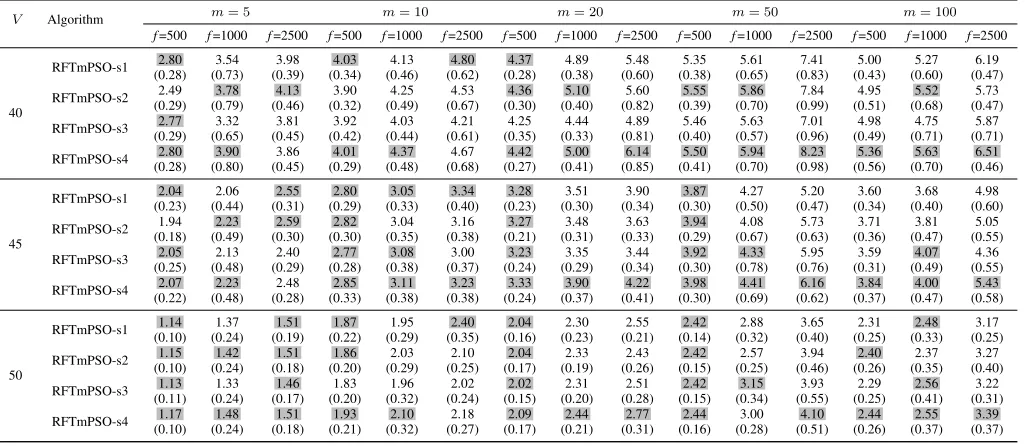
Figure 1 compares the true and predicted landscapes in
D=2. Each environment is produced by 2500 points, and the
parameter setting of mMPBR is based on default values in Table I withm=5. The first 15 environments are used to train the predictor [6], [8]. Figure 1 shows that the error of the predictor is noticeable even though the true fitness values in previous environments are used to train it.
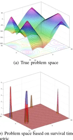
As can be seen in Table VII, ROOT-TFV has the highest average survival time in test instances with D=2 but loses its superiority in problems with D=5 and its performance, as well as that of ROOT-PV, experience a dramatic drop. To understand why these two methods struggle with even moderately dimensional problems, one has to note that they use (8) as fitness instead of the true fitness function (22). Figure 2 visualizes an example of the search space according to (8) in D=2. Figure 2(a) shows the true fitness landscape according to (22) and Fig. 2(b) shows the corresponding environment based on (8) withV=40 and its true five future environments. As can be seen, most of the problem landscapes defined by (8) are flat with a few narrow peaks. This is really challenging for the optimizer, especially in higher dimensions. To investigate the performance of PSO in this type of environments, we use PSO for optimizing the mMPBR with 5 peaks and 100 environmental changes. This experiment is done 50 times and at the end of each environment, theGbestvalue of PSO based on the environment made by (8) is saved. The averageGbestvalues are reported in Table VIII. Experiments for Table VIII are done on mMPBR in 2, 5 and 10 dimensions and with the number of evaluations per changef of 2500 and 10000 andV = 40.
(a) 16th true environment (b)17thtrue environment (c)18th true environment
[image:12.612.119.495.61.275.2](d)16thpredicted environment (e)17th predicted environment (f)18thpredicted environment
Fig. 1. An example of mMPBR in dimensionD=2 to show the error of the predictor.
(a) True problem space
(b) Problem space based on survival time metric
Fig. 2. The search space made by (8) with a threshold V=40, dimension
D=2 and peak numberm=5 versus the true problem space.
TABLE VIII
AVERAGEGBEST VALUE(STANDARD ERROR IN PARENTHESIS)OFPSOIN SEARCH SPACE MADE BY(8)WITH DIFFERENT DIMENSIOND.
Parameter settings D=2 D=5 D=10
Population size=50,f=2500 5.02(0.17) 2.78(0.32) 0(0) Population size=100,f=10000 5.31(0.16) 3.42(0.27) 0(0)
significantly and the results show that they are not able to find the best peak. Furthermore, the difference between the first and the second PSO increases relatively to their results inD= 2. This shows that the PSO needs more particles and
time to deal with this type of environment. PSO fails to find peaks inD= 10.
Given the results in Table VIII and the fact that the search environment is shaped by the survival time metric (8) (an example is shown in Fig. 2(b)), we conclude that with increas-ing dimension, the search space becomes very challengincreas-ing for optimizers using the survival time metric (8). This was confirmed in [11] where ROOT methods based on (8) have poor performance in higher dimensions. Our analysis provides an explanation for this behavior.
Table VII shows that the performance of FTmPSO, designed for TMO but used as ROOT algorithm, is better than ROOT-PV in most test instances and works surprisingly well at find-ing robust solutions. The only other paper that has investigated the performance of population-based algorithms designed for TMO in the context of ROOT is [6], and according to the reported results and analysis in this paper, some TMO algorithms also succeeded in finding robust solutions in ROOT. The reason behind the acceptable performance of some TMO based algorithms in ROOT is that in most research in the DOP domain, researchers have been working on DOPs with small changes, where the obtained knowledge from the current environment is useful for improving the optimization process in the next environment. In this type of environments which were also used in most ROOT papers, solutions around the peak centers can be robust solutions. Indeed, when comparing Fig. 2(a) and Fig. 2(b), it can be seen that robust solutions are around peak centers.
[image:12.612.113.238.320.559.2] [image:12.612.56.292.638.677.2]problems withD=2. The average fitness value (11) of robust solutions obtained by the TMO algorithm is the best in all test instances because this algorithm chooses the best found solution in terms of fitness value.
For all three methods based on the proposed ROOT frame-work, the average fitness value of robust solutions in all test instances are better than that of ROOT-PV and ROOT-TFV because the proposed methods search the problem space with actual fitness values and choose one of the peaks as robust solution. On the other hand, ROOT-PV and ROOT-TFV use the survival time metric and thus can get stuck in flat areas (Fig. 2(b)). For the same reason, their average fitness value can be very poor in problems with higherDandV (e.g. these two algorithms achieve negative average fitness values inD=5,
m=5).
In this section, we embedded three different multi-swarm methods in the proposed ROOT framework. The reported results in Table VII show that the proposed algorithms are able to perform better than previous state-of-the-art survival time metric (8) based methods especially on the environments with higher number of dimensions.
Comparing results of RFTmPSO-s4, RAmQSO-s4 and RmNAFSA-s4, we realize that the quality of swarms in finding and tracking peaks can improve the proposed frameworks performance noticeably. Specifically, better peak finding and tracking performance corresponds to more accurate informa-tion (gathered by (15), (16) and (17)) leading to more reliable decision making by (18), (19), (20) and (21).
VI. CONCLUSION
A new framework for robust optimization over time (ROOT) was proposed. In the proposed framework, a multi-swarm/multi-population method is responsible for finding, tracking and monitoring peaks. Each sub-swarm gathers in-formation about its covered peak. This inin-formation is used to predict the future behavior of the peak and pick the next robust solution in case the current solution becomes unacceptable. We used three types of information based on shift severity, height variance and fitness variance of peaks and designed four different solution selection strategies based on this information. The experimental results show that the fourth strategy that uses the information about shift severity as well as height variance of peaks had the best performance overall and can be used for other problem instances.
We used a wide range of problem settings to investigate the performance of the proposed framework based algorithms versus the existing state-of-the-art framework based on a sur-vival time metric. We showed that the performance of previous methods that use the survival time metric is substantially worse in problems with higher dimensions. All previous state-of-the-art methods attempt to predict future fitness values of solutions based on previous fitness values of solutions. However, this is a difficult task and can become almost impossible for problems with higher dimensions, larger search space and higher change frequencies. In our experiments, we thus investigate the considerable effect of predictor errors and approximation errors on the performance of previous
methods. On the other hand, our proposed framework does not have to deal with the challenges of predicting future fitness values. The experimental results show that the performance of the proposed framework is significantly better than that of state-of-the-art methods especially in problems with higher dimensions.
We tested the proposed framework based algorithms on problem instances with different combinations of parameter settings of mMPBR and provided performance analysis based on them. The results showed that the problem becomes more challenging when shift severities of peaks, dimension of problem space, and change frequency are higher. However, the reported results showed that the proposed methods were able to perform very well even in more challenging problems. Future work will include a study of other peaks behavioral information and design of new strategies for choosing robust solutions. Additionally, other objectives of robust optimization over time such as minimizing solution change cost will be investigated. Another interesting area is ROOT for DOPs with undetectable changes [36]. Finally, we will investigate the performance of the proposed framework on other types of problems including real-world applications.
ACKNOWLEDGEMENTS
The authors would like to thank Dr. Mohammad Nabi Omidvar for the valuable discussions and his constructive feedback.
REFERENCES
[1] T. T. Nguyen, S. Yang, and J. Branke, “Evolutionary dynamic opti-mization: A survey of the state of the art,” Swarm and Evolutionary Computation, vol. 6, pp. 1–24, 2012.
[2] D. E.Wilkins, S. F.Smith, L. A.Kramer, T. J.Lee, and T. W.Rauenbusch, “Airlift mission monitoring and dynamic rescheduling,” Engineering Applications of Artificial Intelligence, vol. 21, no. 2, pp. 141–155, 2008. [3] J. A. D. Atkin, E. K. Burke, J. S. Greenwood, and D. Reeson, “On-line decision support for take-off runway scheduling with uncertain taxi times at london heathrow airport,”Journal of Scheduling, vol. 11, no. 5, pp. 323–346, 2008.
[4] X. Yu, Y. Jin, K. Tang, and X. Yao, “Robust optimization over time - a new perspective on dynamic optimization problems,” inIEEE Congress on Evolutionary Computation (CEC). IEEE, 2010, pp. 1–6. [5] H. Fu, B. Sendhoff, K. Tang, and X. Yao, “Characterizing
environmen-tal changes in robust optimization over time,” in IEEE Congress on Evolutionary Computation (CEC). IEEE, 2012, pp. 1–8.
[6] Y. Jin, K. Tang, X. Yu, B. Sendhoff, and X. Yao, “A framework for finding robust optimal solutions over time,”Memetic Computing, vol. 5, no. 01, pp. 3–18, 2013.
[7] J. Kennedy and R. Eberhart, “Particle swarm optimization,” in Inter-national Conference on Neural Networks, vol. 04. IEEE, 1995, pp. 1942–1948.
[8] H. Fu, B. Sendhoff, K. Tang, and X. Yao, “Finding robust solutions to dynamic optimization problems,” in Applications of Evolutionary Computation, vol. 7835. Lecture Notes in Computer Science, 2013, pp. 616–625.
[9] H. Fu, B. Sendhoff, K. Tang, and X. Yao, “Robust optimization over time: problem difficulties and benchmark problems,”IEEE Transactions on Evolutionary Computation, vol. 19, no. 5, pp. 731–745, 2015. [10] Y. nan Guo, M. Chen, H. Fu, and Y. Liu, “Find robust solutions over time
by two-layer multi-objective optimization method,” inIEEE Congress on Evolutionary Computation (CEC). IEEE, 2014, pp. 1528–1535. [11] Y. Huang, Y. Ding, K. Hao, and Y. Jin, “A multi-objective approach to
robust optimization over time considering switching cost,”Information Sciences, vol. 394-395, pp. 183–197, 2017.
[13] M. Mavrovouniotis, C. Li, and S. Yang, “A survey of swarm intelligence for dynamic optimization: Algorithms and applications,” Swarm and Evolutionary Computation, vol. 33, pp. 1–17, 2017.
[14] J. Branke, T. Kaussler, C. Smidt, and H. Schmeck, “A multipopulation approach to dynamic optimization problems,” inEvolutionary Design and Manufacture, 2000, pp. 299–307.
[15] D. Yazdani, B. Nasiri, R. Azizi, A. Sepas-Moghaddam, and M. R. Meybodi, “Optimization in dynamic environments utilizing a novel method based on particle swarm optimization,” International Journal of Artificial Intelligence, vol. 11, pp. 170–192, 2013.
[16] C. Li and S. Yang, “Optimization in dynamic environments utilizing a novel method based on particle swarm optimization,” in4th International Conference on Natural Computation. IEEE, 2008, pp. 624–628. [17] A. Sepas-Moghaddam, A. Arabshahi, D. Yazdani, and M. M. Dehshibi,
“A novel hybrid algorithm for optimization in multimodal dynamic en-vironments,” inInternational Conference on Hybrid Intelligent Systems (HIS). IEEE, 2012, pp. 143–148.
[18] B. Nasiri, M. R. Meybodi, and M. M. Ebadzadeh, “History-driven particle swarm optimization in dynamic and uncertain environments,”
Neurocomputing, vol. 172, pp. 356–370, 2016.
[19] D. Yazdani, A. Sepas-Moghaddam, A. Dehban, and N. Horta, “A novel approach for optimization in dynamic environments based on modified artificial fish swarm algorithm,”International Journal of Computational Intelligence and Applications, vol. 15, no. 02, pp. 1 650 010–1 650 034, 2016.
[20] D. Yazdani, B. Nasiri, A. Sepas-Moghaddam, M. R. Meybodi, and M. Akbarzadeh-Totonchi, “mNAFSA: A novel approach for optimiza-tion in dynamic environments with global changes,”Swarm and Evolu-tionary Computation, vol. 18, pp. 38–53, 2014.
[21] D. Yazdani, M. R. Akbarzadeh-Totonchi, B. Nasiri, and M. R. Meybodi, “A new artificial fish swarm algorithm for dynamic optimization prob-lems,” inIEEE Congress on Evolutionary Computation (CEC). IEEE, 2012, pp. 1–8.
[22] D. Parrott and X. Li, “Locating and tracking multiple dynamic optima by a particle swarm model using speciation,” IEEE Transactions on Evolutionary Computation, vol. 10, no. 04, pp. 440–458, 2006. [23] S. Bird and X. Li, “Using regression to improve local convergence,” in
IEEE Congress on Evolutionary Computation. IEEE, 2007, pp. 592– 599.
[24] C. Li and S. Yang, “A clustering particle swarm optimizer for dynamic optimization,” inIEEE Congress on Evolutionary Computation. IEEE, 2009, pp. 439–446.
[25] S. Yang and C. Li, “A clustering particle swarm optimizer for locating and tracking multiple optima in dynamic environments,”IEEE Transac-tions on Evolutionary Computation, vol. 14, no. 06, pp. 959–974, 2010. [26] W. Du and B. Li, “Multi-strategy ensemble particle swarm optimization for dynamic optimization,”Information Sciences, vol. 178, no. 15, pp. 3096–3109, 2008.
[27] T. Blackwell and J. Branke, “Multiswarms, exclusion, and anti-convergence in dynamic environments,”IEEE Transactions on Evolu-tionary Computation, vol. 10, no. 4, pp. 459–472, 2006.
[28] T. Blackwell, J. Branke, and X. Li, “Particle swarms for dynamic optimization problems,” inSwarm Intelligence: Introduction and Ap-plications, C. Blum and D. Merkle, Eds. Springer, 2008, pp. 193–217. [29] C. Li, T. T. Nguyen, M. Yang, M. Mavrovouniotis, and S. Yang, “An adaptive multi-population framework for locating and tracking multiple optima,” IEEE Transactions on Evolutionary Computation, vol. 20, no. 05, pp. 590–605, 2016.
[30] D. Yazdani, B. Nasiri, A. Sepas-Moghaddam, and M. R. Meybodi, “A novel multi-swarm algorithm for optimization in dynamic environments based on particle swarm optimization,”Applied Soft Computing, vol. 13, no. 04, pp. 2144–2158, 2013.
[31] D. Yazdani, T. T. Nguyen, J. Branke, and J. Wang, “A multi-objective time-linkage approach for dynamic optimization problems with previous-solution displacement restriction,” inEuropean Conference on the Applications of Evolutionary Computation, K. Sim and P. Kaufmann, Eds. Lecture Notes in Computer Science, 2018, vol. 10784, pp. 864– 878.
[32] T. T. Nguyen, “Continuous dynamic optimisation using evolutionary algorithms,” Ph.D. dissertation, University of Birmingham, Birmingham, UK, 2011.
[33] J. Branke, “Memory enhanced evolutionary algorithms for changing op-timization problems,” inIEEE Congress on Evolutionary Computation. IEEE, 1999, pp. 1875–1882.
[34] D. Yazdani, T. T. Nguyen, J. Branke, and J. Wang, “A new multi-swarm particle multi-swarm optimization for robust optimization over time,” inApplications of Evolutionary Computation, G. Squillero and K. Sim,
Eds. Springer Lecture Notes in Computer Science, 2017, vol. 10200, pp. 99–109.
[35] C. Li, T. T. Nguyen, E. L. Yu, X. Yao, Y. Jin, and H. G. Beyer, “Bench-mark generator for cec 2009 competition on dynamic optimization,” Department of Computer Science, University of Leicester, UK, Tech. Rep., 2009.
[36] C. Li and S. Yang, “A general framework of multipopulation methods with clustering in undetectable dynamic environments,”IEEE Transac-tions on Evolutionary Computation, vol. 16, no. 4, pp. 556–577, 2012.
Danial Yazdani received his BSc in 2007 from Shirvan Azad University, and his MSc in 2011 from Qazvin Azad University in computer science. Cur-rently, he is a PhD student at Liverpool John Moores University. His main research interests include dif-ferent types of dynamic optimization problems such as constrained, time-linkage, multi-objective, large-scale, and combinatorial. He has published more than 20 papers in peer-reviewed journals and con-ferences.
Trung Thanh Nguyen received his BSc in 2000 from Vietnam National University, and his MPhil and PhD in Computing Science from University of Birmingham in 2007 and 2011, respectively. He has been a Reader in Operational Research at Liverpool John Moores University (LJMU) since 2015. Prior to that, he was a Senior Lecturer in Optimisation and Simulation Modelling at LJMU since 2013, and a Research Fellow at LJMU and University of Birmingham in 2011. His current research interests include operational research/dynamic optimisation with a particular application to logistics/transport problems.
He is currently the principal investigator of four research grants in transport and logistics. He has published more than 40 peer-reviewed papers. He is/was the chair of three leading conference tracks, member of TPCs of over 30 leading conferences, editor of five books, two journals and invited speaker of various conferences and events.