Co regularised support vector regression

Co-Regularised Support Vector Regression

Katrin Ullrich1, Michael Kamp1,2, Thomas G¨artner3, Martin Vogt1,4, and Stefan Wrobel1,2

1

University of Bonn, Germany

ullrich@iai.uni-bonn.de 2

Fraunhofer IAIS, Sankt Augustin, Germany

michael.kamp@iais.fraunhofer.de, stefan.wrobel@iais.fraunhofer.de

3

University of Nottingham, UK

thomas.gaertner@nottingham.ac.uk 4

B-IT, LIMES Program Unit, Bonn, Germany

martin.vogt@bit.uni-bonn.de

Abstract. We consider a semi-supervised learning scenario for regression, where only few labelled examples, many unlabelled instances and different data rep-resentations (multiple views) are available. For this setting, we extend support vector regression with a co-regularisation term and obtain co-regularised sup-port vector regression (CoSVR). In addition to labelled data, co-regularisation includes information from unlabelled examples by ensuring that models trained on different views make similar predictions. Ligand affinity prediction is an im-portant real-world problem that fits into this scenario. The characterisation of the strength of protein-ligand bonds is a crucial step in the process of drug discovery and design. We introduce variants of the base CoSVR algorithm and discuss their theoretical and computational properties. For the CoSVR function class we pro-vide a theoretical bound on the Rademacher complexity. Finally, we demonstrate the usefulness of CoSVR for the affinity prediction task and evaluate its per-formance empirically on different protein-ligand datasets. We show that CoSVR outperforms co-regularised least squares regression as well as existing state-of-the-art approaches for affinity prediction.

Keywords: regression, kernel methods, semi-supervised learning, multiple views, co-regularisation, Rademacher complexity, ligand affinity prediction

1

Introduction

few labelled protein-ligand pairs, millions of small compounds are gathered in molec-ular databases as ligand candidates. Many different data representations—the so-called molecular fingerprints or views—exist that can be used for learning. Affinity predic-tion and other applicapredic-tions suffer from little label informapredic-tion and the need to choose the most appropriate view for learning. To overcome these difficulties, we propose to apply an approach called co-regularised support vector regression. We are the first to investigate support vector regression with co-regularisation, i.e., a term penalising the deviation of predictions on unlabelled instances. We investigate two loss functions for the co-regularisation. In addition to variants of our multi-view algorithm with a reduced number of optimisation variables, we also derive a transformation into a single-view method. Furthermore, we prove upper bounds for the Rademacher complexity, which is important to restrict the capacity of the considered function class to fit random data. We will show that our proposed algorithm outperforms affinity prediction baselines.

The strength of a protein-compound binding interaction is characterised by the real-valued binding affinity. If it exceeds a certain limit, the small compound is called a

ligandof the protein. Ligand-based classification models can be trained to distinguish

between ligands and non-ligands of the considered protein (e.g., with support vector machines [6]). Since framing the biological reality in a classification setting represents a severe simplification of the biological reality, we want to predict the strength of bind-ing usbind-ing regression techniques from machine learnbind-ing. Both classification and regres-sion methods are also known under the name of ligand-based virtual screening. (In the context of regression, we will use the nameligandsfor all considered compounds.) Various approaches likeneural networks[7] have been applied. However,support

vec-tor regression(SVR) is the state-of-the-art method for affinity prediction studies (e.g.,

[12]).

As mentioned above, in the context of affinity prediction one is typically faced with the following practical scenario: for a given protein, only few ligands with experimen-tally identified affinity values are available. In contrast, the number of synthesizable compounds gathered in molecular databases (such as ZINC, BindingDB, ChEMBL5) is huge which can be used as unlabelled instances for learning. Furthermore, different free or commercial vectorial representations ormolecular fingerprintsfor compounds exist. Originally, each fingerprint was designed towards a certain learning purpose and, there-fore, comprises a characteristic collection of physico-chemical or structural molecular features [1], for example, predefined key properties (Maccs fingerprint) or listed sub-graph patterns (ECFP fingerprints).

The canonical way to deal with multiple fingerprints for virtual screening would be to extensively test and compare different fingerprints [6] or perform time-consuming preprocessing feature selection and recombination steps [8]. Other attempts to utilise multiple views for one prediction task can be found in the literature. For example, Ullrich et al. [13] apply multiple kernel learning. However, none of these approaches include unlabelled compounds in the affinity prediction task. The semi-supervised

co-regularised least squares regression(CoRLSR) algorithm of Brefeld et al. [4] has been

shown to outperform single-viewregularised least squares regression(RLSR) for UCI

datasets6. Usually, SVR shows very good predictive results having a lower general-isation error compared to RLSR. Aside from that, SVR represents the state-of-the-art in affinity prediction (see above). For this reason, we define co-regularised

sup-port vector regression (CoSVR) as an ε-insensitive version of co-regularisation. In

general, CoSVR—just like CoRLSR—can be applied on every regression task with multiple views on data as well as labelled and unlabelled examples. However, learn-ing scenarios with high-dimensional sparse data representations and very few labelled examples—like the one for affinity prediction—could benefit from approaches using co-regularisation. In this case, unlabelled examples can contain information that could not be extracted from a few labelled examples because of the high dimension and spar-sity of the data representation.

A view on data is a representation of its objects, e.g., with a particular choice of features in IRd. We will see that feature mappings are closely related to the concept

of kernel functions, for which reason we introduce CoSVR theoretically in the

gen-eral framework of kernel methods. Within the research field of multi-view learning, CoSVR and CoRLSR can be assigned to the group of co-training style [16] approaches that simultaneously learn multiple predictors, each related to a view. Co-training style approaches enforce similar outcomes of multiple predictor functions for unlabelled ex-amples, measured with respect to some loss function. In the case of co-regularisation for regression the empirical risks of multiple predictors (labelled error) plus an error term for unlabelled examples (unlabelled error, co-regularisation) are minimised.

The idea for mutual influence of multiple predictors appeared in the paper of Blum and Mitchell [2] on classification with co-training. Wang et al. [14] combined the tech-nique of co-training with SVR with a techtech-nique different from co-regularisation. Anal-ogous to CoSVR, CoRLSR is a semi-supervised and multi-view version of RLSR that requires the solution of a large system of equations [4]. A co-regularised version for sup-port vector machine classification SVM-2K already appeared in the paper of Farquhar et al. [5], where the authors define a co-regularisation term via theε-insensitive loss on labelled examples. It was shown by Sindhwani and Rosenberg [11] that co-regularised approaches applying the squared loss function for the unlabelled error can be trans-formed into a standard SVR optimisation with a particular fusion kernel. A bound on the empirical Rademacher complexity for co-regularised algorithms with Lipschitz con-tinuous loss function for the labelled error and squared loss function for the unlabelled error was proven by Rosenberg and Bartlett [9].

A preliminary version of this paper was published at theData Mining in Biomedical

Informatics and Healthcareworkshop held at ICDM 2016. There, we considered only

the CoSVR special caseε-CoSVR and its variants with reduced numbers of variables (for the definitions consult Defs.1-3below) focusing the application of ligand affinity prediction. The `2-CoSVR case (see below) with its theoretical properties (Lemmas 1(ii)-3(ii),6(ii)) and practical evaluation, as well as the fasterΣ-CoSVR (Sect.3.3) variant are novel contributions in the present paper.

In the following section, we will present a short summary of kernels and multiple views, as well as important notation. We define CoSVR and variants of the base al-gorithm in Sect.3. In particular, a Rademacher bound for CoSVR will be proven in

Sect.3.5. Subsequently, we provide a practical evaluation of CoSVR for ligand affinity prediction in Sect.4and conclude with a brief discussion in Sect.5.

2

Kernels and Multiple Views

We consider an arbitrary instance spaceX and the real numbers as label spaceY. We want to learn a functionf that predicts a real-valued characteristic of the elements of X. Suppose for training purposes we have setsX={x1, . . . , xn} ⊂ Xof labelled and Z ={z1, . . . , zm} ⊂ Xof unlabelled instances at our disposal, where typicallymn holds true. With{y1, . . . , yn} ⊂ Ywe denote the respective labels ofX. Furthermore, assume the data instances can be represented inM different ways. More formally, for v ∈ {1, . . . , M}there are functionsΦv :X → Hv, whereHvis an appropriate inner product space. Given an instancex ∈ X, we say thatΦv(x)is thev-th viewof x. If HvequalsIRdfor some finite dimensiond, the intuitive names(v-th) feature mapping

andfeature space are used forΦv andHv, respectively. If in the more general case

Hv is aHilbert space, dcan even be infinite (see below). For view v the predictor

functionfv : X → IRis denoted with (single) view predictor. View predictors can be learned independently for each view utilising an appropriate regression algorithm like SVR or RLSR. As a special case we considerconcatenated predictorsfv in Sect. 4 where the corresponding viewv results from a concatenation of finite dimensional feature representationsΦ1, . . . , ΦM. Having different views on the data, an alternative is to learn M predictorsfv : X → IR simultaneously that depend on each other, satisfying an optimisation criterion involving all views at once. Such a criterion could be the minimisation of the labelled error in line with co-regularisation which will be specified in the following subsection. The final predictorf will then be the average of the predictorsfv.

A functionk:X ×X →IRis said to be akernelif it is symmetric and positive semi-definite. Indeed, for every kernelkthere is a feature mappingΦ : X → Hsuch that

His areproducing kernel Hilbert space(RKHS) and k(x1, x2) = hΦ(x1), Φ(x2)iH

holds true for allx1, x2 ∈ X (Mercer’s theorem). Thus, the functionk is the corre-sponding reproducing kernel ofH, and forx∈ X the mappingshΦ(x), Φ(·)i=k(x,·)

are functions defined onX. Choosing RKHSsHvof multiple kernelskv as candidate spaces for the predictorsfv, therepresenter theoremof Sch¨olkopf et al. [10] allows for a parameterisation of the optimisation problems for co-regularisation presented below. A straightforward modification of the representer theorem’s proof leads to a represen-tation of the predictorsfvas finite kernel expansion

fv(·) =

n X

i=1

πvikv(xi,·) +

m X

j=1

πv(j+n)kv(zj,·) (1)

with linear coefficientsπv ∈IRn+m, centered at labelled and unlabelled instancesxi∈ Xandzj∈Z, respectively.

The kernel matricesKv = {kv(xi, xj)} n+m

will consider the submatrices k(Z, x) := (k(z1, x), . . . , k(zm, x))T andk(Z, Z) := {k(zj, zj0)}_j,jm0₌₁of a Gram matrix with kernelk. IfH1andH2are RKHSs then their sum spaceHΣis defined asHΣ :={f :f =f1+f2, f1∈ H1, f2∈ H2}. WithY =

(y1, . . . , yn)T ∈IRnwe denote the vector of labels. We will abbreviatev∈ {1, . . . , M} withv ∈[[M]]. And finally, we will utilise the squared loss`2(y, y0) = ky−y0k2and theε-insensitive loss`ε(y, y0) = max{0,|y−y0| −ε},y, y0 ∈ Y.

3

The CoSVR Algorithm: Variants and Properties

3.1 Base CoSVR

In order to solve a regression task in the presence of multiple viewsv = 1, . . . , M, the approach ofco-regularisationis to jointly minimise two error terms involvingM predictor functions f1, . . . , fM. Firstly, every view predictor fv is intended to have a small training error with respect to labelled examples. Secondly, the difference between pairwise view predictions over unlabelled examples should preferably be small. We introduce co-regularised support vector regression(CoSVR) as an ε-insensitive loss realisation of the co-regularisation principle.

Definition 1. Forv∈ {1, . . . , M}letHvbe RKHSs. The co-regularised empirical risk

minimisation

min

fv∈Hv M X

v=1 νv

2kfvk

2₊ n X

i=1

`L(yi, fv(xi))

!

(2)

+λ M X

u,v=1 m X

j=1

`U(fu(zj), fv(zj)),

whereνv, λ ≥ 0is called co-regularised support vector regression (CoSVR) if `L =

`εL,εL ≥ 0, and `U is an arbitrary loss function for regression. Furthermore, we

defineε-CoSVR to be the special case where`U <sub>=`</sub>

εU,εU ≥0, as well as`₂-CoSVR

to satisfy`U <sub>=`</sub>

2.

The minimum in (2) is taken over allfv,v = 1, . . . , M. For reasons of simplification we will abbreviateminf1∈H1,...,fM∈HM withminfv∈Hv. Note that the loss function parametersεLandεU can have different values. The parametersνvandλare trade-off parameters between empirical risk and co-regularisation term. The added norm terms kfvkprevent overfitting. We will also refer to the empirical risk term with loss function

`L<sub>aslabelled errorand to the co-regularisation term with`</sub>U_{asunlabelled error. In the}

case of`L <sub>=`</sub>U _=`

2, the optimisation in (2) is known asco-regularised least squares

regression(CoRLSR). Brefeld et al. [4] found a closed form solution for CoRLSR as

linear system of equations inM(n+m)variables. In the following, we present a solu-tion forε-CoSVR and`2-CoSVR.

Lemma 1. Letνv, λ, εL_{, ε}U _{≥0. We use the notation introduced above. In particular,}

from (1), whereasαv,αˆv∈IRnandγuv ∈IRmare dual variables.

(i)The dual optimisation problem ofε-CoSVR equals

max

αv,αˆv∈IRn,γuv∈IRm M X v=1 − 1 2νv _α γ T v Kv _α γ v

+ (αv−αvˆ )TY

−(αv+ ˆαv)TεL1n− M X

u=1

γ_uvT εU1m !

s.t.

0n≤αv,αˆv≤1n

0m≤γuv≤λ1m

v∈[[M]],(u,v)∈[[M]]2

,

whereπ_vT = _ν1

v(α|γ) T

v and(α|γ) T

v = (αv−αvˆ | PM

u=1(γuv−γvu)) T_.

(ii)The dual optimisation problem of`2-CoSVR is

max

αv,αvˆ ∈IRn_,γuv∈IRm M X

v=1 − 1

2νv _α γ T v Kv _α γ v

+ (αv−αvˆ )TY

−εL(αv+ ˆαv)T1n−

1 4λ

M X

u=1 γT_uvγuv

!

s.t.

₀

n ≤αv,αvˆ ≤1n γuv =2_νuλUu α_γ

u−

2λ νvUv

α γ

v

v∈[[M]],(u,v)∈[[M]]2

,

whereπT

v = νv1(α|γ) T

v and(α|γ)Tv = (αv−αˆv| P M

u=1(γuv−γvu))T.

Remark 1. The proofs of Lemma 1 as well as Lemmas2 and3 below use standard

techniques fromLagrangian dualisation(e.g., [3]). They can be found in our CoSVR repository (see footnote7).

We choose the concatenated vector representation(α|γ)T v ∈IR

n+m_{in order to show} the correspondence between the two problems ε-CoSVR and`2-CoSVR and further CoSVR variants below. Additionally, the similarities with and differences to the original SVR dual problem are obvious. We will refer to the optimisation in Lemma1as the base CoSVR algorithms.

3.2 Reduction of Variable Numbers

Modification of the Empirical Risk In base CoSVR the empirical risk is meant to be small for each single view predictor individually using examples and their correspond-ing labels. In the CoSVRmod_{variant the average prediction, i.e., the final predictor, is} applied to define the labelled error term.

Definition 2. The co-regularised support vector regression problem with modified

con-straints for the labelled examples (CoSVRmod) is defined as

min

fv∈Hv M X

v=1 νv

2 kfvk

2₊ n X

i=1

`_εL(yi, favg(xi))

+λ M X u,v=1 m X j=1

`U(fu(zj), fv(zj)),

wherefavg _:= 1

M PM

v=1fvis the average of all single view predictors. We denote the

case`U <sub>=`</sub>

εU,εU ≥0, withε-CoSVRmodand the case`U =`₂with`₂-CoSVRmod.

In the following lemma we present solutions forε-CoSVRmodand`2-CoSVRmod.

Lemma 2. Letνv, λ, εL_{, ε}U _{≥0. We utilise dual variablesα,αˆ∈IR}n_{andγuv ∈IR}m_.

(i)Theε-CoSVRmod_{dual optimisation problem can be written as}

max

α,αˆ∈IRn_{, γuv∈IR}m M X v=1 − 1 2νv α γ T v Kv α γ v

+ (α−αˆ)TY

−(α+ ˆα)TεL1n− M X

u=1

γ_uvT εU1m !

s.t.

0n ≤α,αˆ≤1n

0m≤γuv ≤λ1m

v∈[[M]] ,

whereπT

v = νv1(α|γ) T

v and(α|γ)Tv = (M1(α−αˆ)| PM

u=1(γuv−γvu))T.

(ii)The`2-CoSVRmoddual optimisation problem equals

max

α,αˆ∈IRn_{, γuv∈IR}m M X

v=1 − 1

2νv _α γ T v Kv _α γ v

+ (αv−αvˆ )TY

−(αv+ ˆαv)TεL1n−

1 4λ

M X

u=1 γ_uvT γuv

!

s.t.

₀

n ≤α,αˆ≤1n γuv =2νλuUu

α γ

u− 2λ νvUv

α γ

v

v∈[[M]] ,

whereπT

v = 1 νv(α|γ)

T

v and(α|γ)Tv = ( 1

M(α−αˆ)| PM

u=1(γuv−γvu))T.

Modification of the Co-Regularisation The unlabelled error term of base CoSVR bounds the pairwise distances of view predictions, whereas now in CoSVRmodonly the disagreement between predictions of each view and the average prediction of the residual views will be taken into account.

Definition 3. We consider RKHSsH1, . . . ,HM as well as constantsεL, εU, νv, λ≥0.

The co-regularised support vector regression problem with modified constraints for the

unlabelled examples (CoSVRmod) is defined as

min

fv∈Hv M X

v=1 νv

2 kfvk

2₊ n X

i=1

`εL(y_i, f_v(x_i)) ! (3) +λ M X v=1 m X j=1

`U(fvavg(zj), fv(zj)),

where nowfavg

v :=M1−1

PM,u6=v

u=1 fuis the average of view predictors besides viewv.

We denote the case`U <sub>=`</sub>

εU,εU ≥0, withε-CoSVRmodand the case`U =`2with

`2-CoSVRmod.

Again we present solutions forε-CoSVRmodand`2-CoSVRmod.

Lemma 3. Letνv, λ, εL, εU ≥0. We utilise dual variablesαv,αvˆ ∈IRnandγv,ˆγv ∈

IRm, as well asγvavg := M1−1

PM,u6=v

u=1 γuandˆγ avg

v := M1−1

PM,u6=v

u=1 ˆγuanalogous

to the residual view predictor average.

(i)Theε-CoSVRmoddual optimisation problem can be written as

max

αv,αˆv∈IRn, γv,γˆv∈IRm M X v=1 − 1 2νv _α γ T v Kv _α γ v

+ (α−αˆ)TY

−(αv+ ˆαv)TεL1n−(γv+ ˆγv)εU1m

s.t.

0n≤αv,αvˆ ≤1n

0m≤γv,ˆγv≤λ1m

v∈[[M]] ,

whereπvT = ν1v(α|γ) T

v and(α|γ)Tv = (αv−αvˆ |(γv−γvavg)−(ˆγv−γˆvavg))T.

(ii)The`2-CoSVRmoddual optimisation problem equals

max

αv,αˆv∈IRn, γv∈IRm M X v=1 − 1 2νv _α γ T v Kv _α γ v

+ (αv−αvˆ )TY

−(αv+ ˆαv)TεL1n−

1 4λ

M X

u=1 γ_vTγv

!

s.t.

(

0n≤αv,αˆv≤1n

γv= _M1₋₁P M,u6=v u=1

2λ νuUu

α γ

u− 2λ νvUv

α γ

v )

v∈[[M]] ,

whereπT

v = νv1(α|γ) T

Remark 2. If we combine the modifications in the labelled and unlabelled error term we canonically obtain the variantsε-CoSVRmod

modand`2-CoSVRmodmod.

In the base CoSVR versions the semi-supervision is realised with proximity constraints on pairs of view predictions. We show in the following lemma that the constraints of the closeness of one view prediction to the average of the residual predictions implies a closeness of every pair of predictions.

Lemma 4. Up to constants, the unlabelled error bound of CoSVRmodis also an upper

bound of the unlabelled error of base CoSVR.

Proof. We consider the settings of Lemma1(i)and Lemma3(i). For part(ii)the proof

is equivalent with εU _{= 0. In the case of M = 2, modified and base algorithm fall} together which shows the claim. Now letM > 2. Because of the definition of the ε-insensitive loss we know that|fv(zj)−fvavg(zj)| ≤ εU +cvj,wherecvj ≥ 0is the actual loss value for fixedvandj. We denotecj := maxv∈{1,...,M}{c1j, . . . , cM j}and, hence,|fv(zj)−favg

v (zj)| ≤ εU +cjfor allv ∈ {1, . . . , M}. Now we conclude for j∈ {1, . . . , m}and(u, v)∈ {1, . . . , M}2

|fu(zj)−fv(zj)|

≤ |fu(zj)−f_uavg(zj)|+|f_uavg(zj)−f_vavg(zj)|+|f_vavg(zj)−fv(zj)|

≤εU+cj+_M1₋₁|fv(zj)−fu(zj)|+εU +cj,

and therefore,|fu(zj)−fv(zj)| ≤ 2(M−1)

M−2 (ε U_+c

j).As a consequence we deduce from PM

v=1 Pm

j=1`εU(f_vavg(zj), fv(zj))≤MPm_j=1cj =:Bthat also the labelled error of CoSVR can be boundedPM

u,v=1 Pm

j=1`ε˜(fu(zj), fv(zj))≤B˜forε˜= 2(M−1)

M−2 ε U_and

˜

B= 2M_(M(M₋₂₎−1)B, which finishes the proof. ut

3.3 Σ-CoSVR

Sindhwani and Rosenberg [11] showed that under certain conditions co-regularisation approaches of two views exhibit a very useful property. If`U <sub>= `</sub>

2and the labelled loss is calculated utilising an arbitrary loss function for the average predictorfavg_, the resulting multi-view approach is equivalent with a single-view approach of a fused kernel. We use the notion from Sect.2.

Definition 4. Letλ, ν1, ν2, εL ≥0be parameters and the Gram submatricesk(Z, x)

andk(Z, Z)be defined as in Sect.2. We consider a merged kernelkΣ from two view

kernelsk1andk2

kΣ(x, x0) :=k⊕(x, x0)−k (Z, x)T λ1Im+k⊕(Z, Z) −1

k (Z, x0), (4)

forx, x0_{∈ X, wherek}⊕_:= 1

ν1k1+

1

ν2k2andk :=

1 ν1k1−

1

ν2k2. We denote the SVR

optimisation

argmin

f∈HΣ

kfk2₊ n X

i=1

`εL(y_i,1

2f(xi)), (5)

Please notice that for each pair(x, x0)the value ofkΣ(x, x0)is calculated in (4) with k1andk2including not onlyxandx0but also unlabelled examplesz1, . . . , zm. Hence, the optimisation problem in (5) is a standard SVR with additional information about unlabelled examples incorporated in the RKHSHΣ.

Lemma 5. The algorithms`2-CoSVRmodandΣ-CoSVR are equivalent andHΣis the

sum spaceHΣ ={f :X →IR|f =f1+f2, f1∈ H1, f2∈ H2}.

Proof. The proof is an application of Theorem 2.2. of Sindhwani and Rosenberg [11]

for the loss functionV being equal to theε-insensitive loss withε=εL_{, the parameter}

of the labelled error of`2-CoSVRmod. ut

AsΣ-CoSVR can be solved as a standard SVR algorithm we obtained a much faster co-regularisation approach. The information of the two views and the unlabelled examples are included in the candidate spaceHΣ and associated kernelkΣ.

3.4 Complexity

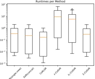
The CoSVR variants and CoRLSR mainly differ in the number of applied loss func-tions and the strictness of constraints. This results in different numbers of variables and constraints in total, as well as potentially non-zero variables (referred to assparsity, compare Table1). All presented problems are convex QPs with positive semi-definite

Table 1: Number of variables, constraints, and potential non-zero variables for differ-ent CoSVR versions and CoRLSR. The respective CoSVRmod variant is included by cancelling the{M}-factor.

algorithm variables constraints sparsity ε-CoSVR 2{M}n+M2_{m 4{M}n+ 2M}2_{m {M}n+}1

2(M

2_−M)m

`2-CoSVR 2{M}n+M2m 4{M}n+M2m {M}n+M2m

ε-CoSVRmod 2{M}n+ 2M m 4{M}n+ 4M m {M}n+M m

`2-CoSVRmod 2{M}n+M m 4{M}n+M m {M}n+M m

Σ-CoSVR 2n 4n n

CoRLSR M n+M m 0 M n+M m

use theε-insensitive loss for the labelled error in all CoSVR versions. And finally, in the two-view case withM = 2the modified version with respect to the unlabelled error term and the base version coincide.

3.5 A Rademacher Bound for CoSVR

Similarly to the result of Rosenberg and Bartlett [9] we want to prove a bound on the

empirical Rademacher complexityRˆn of CoSVR in the case ofM = 2. Note that,

despite the proof holding for the special case ofM = 2, the CoSVR method in general is applicable to arbitrary numbers of views. The empirical Rademacher complexity is a data-dependent measure for the capacity of a function classHto fit random data and is defined as

ˆ

Rn(H) =Eσ "

sup

f∈H

2

n n X

i=1

σif(xi)

:{x1, . . . , xn}=X #

.

The random data are represented viaRademacher random variablesσ= (σ1, . . . , σn)T. We considerε-CoSVR and `2-CoSVR and define bounded versionsHεΣ andHΣ2 of the sum space HΣ from Sect. 2 for the corresponding versions. Obviously, a pair

(π1, π2) ∈ IR(n+m)×(n+m) of kernel expansion coefficients (see (1)) represents an element ofHΣ. Forε-CoSVR and`2-CoSVR we set

Hε

Σ :={(π1, π2)∈ HΣ :−µ1n+m≤π1, π2≤µ1n+m}, and (6) H2

Σ :={(π1, π2)∈ HΣ :ν1πT1K1π1+ν2π2TK2π2

+λ(U1π1−U2π2)T(U1π1−U2π2)≤1 , (7) respectively. In (6)µis an appropriate constant according to Lemma1and2. The def-inition in (7) follows the reasoning of Rosenberg and Bartlett [9]. Now we derive a bound on the empirical Rademacher complexity ofHε

ΣandH 2

Σ, respectively. We point out that the subsequent proof is also valid for the modified versions with respect to the empirical risk. For two views the base and modified versions with respect to the co-regularisation fall together anyway. For reasons of simplicity, in the following lemma and proof we omitmodandmod for the CoSVR variants. Furthermore, we will apply the infinity vector normkvk∞and row sum matrix normkLk∞(consult, e.g., Werner [15]).

Lemma 6. LetHε

Σ andH2Σbe the function spaces in (6) and (7) and, without loss of

generality, letY= [−1,1].

(i)The empirical Rademacher complexity ofε-CoSVR can be bounded via

ˆ

Rn(HεΣ)≤

2s

nµ(kL1k∞+kL2k∞),

whereµis a constant dependent on the regularisation parameters andsis the number

of potentially non-zero variables in the kernel expansion vectorπ∈ Hε

Σ.

(ii)The empirical Rademacher complexity of`2-CoSVR has a bound

ˆ

Rn(H2Σ)≤

2

n p

wheretrn(KΣ) :=P n

i=1kΣ(xi, xi)with the sum kernelkΣfrom (4). Our proof applies Theorem 2 and 3 of Rosenberg and Bartlett [9].

Proof. At first, using Theorem 2 of Rosenberg and Bartlett [9], we investigate the

gen-eral usefulness of the empirical Rademacher complexityRˆn of HlossΣ in the CoSVR scenario. The function spaceHloss

Σ can be eitherHεΣ orH2Σ. Theorem 2 requires two preconditions. First, we notice that theε-insensitive loss function utilising the average predictor`L_{(y, f(x)) = max{0,|y−(f}

1(x)+f2(x))/2|−εL}maps into[0,1]because of the boundedness ofY. Second, it is easy to show that`L<sub>isLipschitz continuous, i.e.</sub> |`L_{(y, y}0_)−`L_{(y, y}00_)|/|y0_−y00_{| ≤C, for some constantC >0. With similar arguments} one can show that theε-insensitive loss function of base CoSVR is Lipschitz continu-ous as well. According to Theorem 2 of Rosenberg and Bartlett [9], the expected loss

E(X,Y)∼D`L(f(X), Y)can then be bounded by means of the empirical risk and the empirical Rademacher complexity

ED`L(f(X), Y)≤

1

n n X

i=1

lL(f(xi), yi) + 2CRˆn(HlossΣ ) +

2 + 3pln(2/δ)/2

√ n

for everyf ∈ Hloss

Σ with probability at least1−δ. Now we continue with the cases(i) and (ii) separately.

(i)We can reformulate the empirical Rademacher complexity

ˆ

Rn(HεΣ) =

2

nE σ

"

sup

(π1|π2)T∈K

σT(L1π1+L2π2) #

,

whereK := {(π1 |π2)T ∈ IR2(n+m) : −µ1n+m ≤ π1, π2 ≤ µ1n+m}. The kernel expansionπofε-CoSVR optimisation is bounded because of the box constraints in the respective dual problems. Therefore,πlies in the`1-ball of dimensionsscaled with sµ, i.e.,π ∈ sµ·B1. The dimensionsis the sparsity ofπ, and thus, the number of expansion variablesπvj different from zero. From the dual optimisation problem we know thats2(n+m). It is a fact thatsup_π∈sµ·B

1|hv, πi|=sµkvk∞(see Theorems

II.2.3 and II.2.4 in Werner [15]). Let L ∈ IRn×2(n+m) be the concatenated matrix L= (L1|L2), whereL1andL2are the upper parts of the Gram matricesK1andK2 according to Sect.2. From the definition we see thatv=σTLand, hence,

sµkvk∞=sµkσTLk∞≤sµkσk∞kLk∞≤sµkLk∞

=sµ max

i=1,...,n n+m

X

j=1 X

v=1,2

|kv(xi, xj)|.

Finally, we obtain the desired upper bound for the empirical Rademacher complexity ofε-CoSVR

ˆ

Rn(HεΣ)≤

2

nE σ_sµkLk

∞≤

2s

nµ(kL1k∞+kL2k∞).

(ii)Having the Lipschitz continuity of theε-insensitive loss`L_{, the claim is a direct} consequence of Theorem 3 in the work of Rosenberg and Bartlett [9], which finishes

0.0 0.5 1.0 1.5 2.0 2.5 RMSE CoRLSR 0.0

0.5 1.0 1.5 2.0 2.5

RMSE CoSVR

-CoSVR

2-CoSVR

-CoSVR

(a)

0.0 0.5 1.0 1.5 2.0 2.5 RMSE SVR (concat) 0.0

0.5 1.0 1.5 2.0 2.5

RMSE CoSVR

-CoSVR

2-CoSVR

-CoSVR

(b)

0.0 0.5 1.0 1.5 2.0 2.5 RMSE SVR (best) 0.0

0.5 1.0 1.5 2.0 2.5

RMSE CoSVR

-CoSVR

2-CoSVR

-CoSVR

(c)

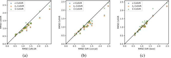
Fig. 1: Comparison of ε-CoSVR, `2-CoSVR, and Σ-CoSVR with the baselines CoRLSR, SVR(concat), and SVR(best) on 24 datasets using the fingerprints Gpi-DAPH3 and ECFP4 in terms of RMSEs. Each point represents the RMSEs of the two methods compared on one dataset.

4

Empirical Evaluation

In this section we evaluate the performance of the CoSVR variants for predicting the affinity values of small compounds against target proteins.

Our experiments are performed on24datasets consisting of ligands and their affinity to one particular human protein per dataset, gathered from BindingDB. Every ligand is a single molecule in the sense of a connected graph and all ligands are available in the standard molecular fingerprint formats ECFP4, GpiDAPH3, and Maccs. All three formats are binary and high-dimensional. An implementation of the proposed methods and baselines, together with the datasets and experiment descriptions are available as open source7_.

We compare the CoSVR variants ε-CoSVR, `2-CoSVR, and Σ-CoSVR against CoRLSR, as well as SVR with a single-view (SVR([fingerprint name])) in terms of root mean squared error (RMSE) using the linear kernel. We take the two-view setting in our experiments as we want to includeΣ-CoSVR results in the evaluation. Another natural baseline is to apply SVR to a new view that is created by concatenating the features of all views (SVR(concat)). We also compare the CoSVR variants against an oracle that chooses the best SVR for each view and each dataset (SVR(best)) by taking the result with the best performance in hindsight.

We consider affinity prediction as semi-supervised learning with many unlabelled data instances. Therefore, we split each labelled dataset into a labelled (30%of the ex-amples) and an unlabelled part (the remaining70%). For the co-regularised algorithms, both the labelled and unlabelled part are employed for training, i.e., in addition to la-belled examples they have access to the entire set of unlala-belled instances without labels. Of course, the SVR baselines only consider the labelled examples for training. For all algorithms the unlabelled part is used for testing. The RMSE is measured using 5-fold

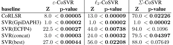
Table 2: Comparing RMSEs using Wilcoxon signed-rank test (hypothesis test on whether CoSVR has significantly smaller RMSEs than the baselines).

ε-CoSVR `2-CoSVR Σ-CoSVR

baseline Z p-value Z p-value Z p-value CoRLSR 8.0 <0.00005 13.0<0.00009 70.0<0.02226

SVR(GpiDAPH3) 1.0 <0.00002 1.0 <0.00002 1.0 <0.00002

SVR(ECFP4) 22.5<0.00027 44.0<0.00738 94.0 <0.1096

SVR(concat) 3.0 <0.00003 24.0<0.00032 79.5<0.04397

SVR(best) 27.0<0.00044 56.0<0.02208 88.0 <0.07649

cross-validation. The parameters for each approach on each dataset are optimised using grid search with 5-fold cross-validation on a sample of the training set.

In Fig.1we present the results of the CoSVR variants compared to CoRLSR(a), SVR(concat)(b), and SVR(best)(c)for all datasets using the fingerprints GpiDAPH3 and ECFP4. Fig.1 (a),(b)indicate that all CoSVR variants outperform CoRLSR and SVR(concat) on the majority of datasets. Fig.1 (c)indicates that SVR(best) performs better than the other baselines but is still outperformed byε-CoSVR and`2-CoSVR. Σ-CoSVR performs similar to SVR(best).

The indications in Fig.1are substantiated by a Wilcoxon signed-rank teston the results (presented in Table2). In this table, we report the test statistics (Zandp-value). Results in which a CoSVR variant statistically significantly outperforms the baselines (for a significance levelp <0.05) are marked in bold. The test confirms that all CoSVR variants perform statistically significantly better than CoRLSR and SVR(concat). More-over,ε-CoSVR and`2-CoSVR statistically significantly outperform an SVR trained on each individual view as well as taking the best single-view SVR in hindsight. Although Σ-CoSVR performs slightly better than SVR(best), the advantage is not statistically significant.

In Table3we report the average RMSEs of all CoSVR variants, CoRLSR and the single-view baselines for all combinations of the fingerprints Maccs, GpiDAPH3, and ECFP4. In terms of average RMSE,ε-CoSVR and`2-CoSVR outperform the other ap-proaches for the view combination Maccs and GpiDAPH3, as well as GpiDAPH3 and ECFP4. For the views Maccs and ECFP4, these CoSVR variants have lower average RMSE than CoRLSR and the single-view SVRs. However, for this view combination, the SVR(best) baseline outperforms CoSVR. Note that SVR(best) is only a hypothet-ical baseline, since the best view varies between datasets and is thus unknown in ad-vance. TheΣ-CoSVR performs on average similar to CoRLSR and the SVR(concat) baseline and slightly worse than SVR(best). To avoid confusion about the different per-formances ofΣ-CoSVR and`2-CoSVR, we want to point out thatΣ-CoSVR equals `2-CoSVRmod(see Lemma5) and not`2-CoSVR (equivalent with`2-CoSVRmodfor M = 2) which we use for our experiments.

In conclusion, co-regularised support vector regression techniques are able to ex-ploit the information from unlabelled examples with multiple sparse views in the prac-tical setting of ligand affinity prediction. They perform better than the state-of-the-art single-view approaches [12], as well as a concatenation of features from multi-ple views. In particular,ε-CoSVR and`2-CoSVR outperform the multi-view approach CoRLSR [4] and SVR on all view combinations.`2-CoSVR outperforms SVR(concat) on all,ε-CoSVR on2out of3view combinations. Moreover, both variants outperform SVR(best) on2out of3view combinations.

Table 3: Average RMSEs for all combi-nations of the fingerprints Maccs, Gpi-DAPH3, and ECFP4

Method View Combinations

Maccs, Maccs, GpiDAPH3,

ECFP4 GpiDAPH3 ECFP4

ε-CoSVR 1.035 1.016 1.049

`2-CoSVR 1.007 1.019 1.062 Σ-CoSVR 1.116 1.114 1.151

CoRLSR 1.06 1.073 1.199

SVR(view1) 1.04 1.041 1.355

SVR(view2) 1.094 1.37 1.106

SVR(concat) 1.011 1.12 1.194

SVR(best) 0.966 1.027 1.104

SVR(single-view) SVR(concat)

CoRLSR -CoSVR 2-Co

SVR -CoSVR 103

102

101

100

101

102 Runtimes per Method

Fig. 2: Runtimes of the CoSVR vari-ants, CoRLSR, and single-view SVRs on24ligand datasets and all view com-binations (runtime in log-scale).

5

Conclusion

Bibliography

[1] Bender, A., Jenkins, J.L., Scheiber, J., Sukuru, S.C.K., Glick, M., Davies, J.W.: How Similar Are Similarity Searching Methods? A Principal Component Analysis of Molecular Descriptor Space. J. Chem. Inf. Model. (2009)

[2] Blum, A., Mitchell, T.: Combining Labeled and Unlabeled Data with Co-Training. In: Proceedings of the 11th Annual Conference on Learning Theory (1998) [3] Boyd, S., Vandenberghe, L.: Convex Optimization. Cambridge University Press

(2004)

[4] Brefeld, U., G¨artner, T., Scheffer, T., Wrobel, S.: Efficient Co-Regularised Least Squares Regression. In: Proceedings of the 23rd International Conference on Ma-chine Learning (2006)

[5] Farquhar, J.D.R., Meng, H., Szedmak, S., Hardoon, D., Shawe-Taylor, J.: Two view learning: SVM-2K, Theory and Practice. In: Advances in Neural Information Processing Systems 18 (2006)

[6] Geppert, H., Humrich, J., Stumpfe, D., G¨artner, T., Bajorath, J.: Ligand Prediction from Protein Sequence and Small Molecule Information Using Support Vector Machines and Fingerprint Descriptors. J. Chem. Inf. Model. (2009)

[7] Myint, K.Z., Wang, L., Tong, Q., Xie, X.Q.: Molecular Fingerprint-Based Arti-ficial Neural Networks QSAR for Ligand Biological Activity Predictions. Mol. Pharmaceutics (2012)

[8] Nisius, B., Bajorath, J.: Reduction and Recombination of Fingerprints of Different Design Increase Compound Recall and the Structural Diversity of Hits. Chem. Biol. Drug Des. (2010)

[9] Rosenberg, D.S., Bartlett, P.L.: The Rademacher Complexity of Co-Regularized Kernel Classes. In: Proceedings of the 11th International Conference on Artificial Intelligence and Statistics (2007)

[10] Sch¨olkopf, B., Herbrich, R., Smola, A.J., Williamson, R.: A Generalized Rep-resenter Theorem. In: Proceedings of the Annual Conference on Computational Learning Theory (2001)

[11] Sindhwani, V., Rosenberg, D.S.: An RKHS for Multi-View Learning and Mani-fold Co-Regularization. In: Proceedings of the 25th International Conference on Machine Learning (2008)

[12] Sugaya, N.: Ligand Efficiency-Based Support Vector Regression Models for Pre-dicting Bioactivities of Ligands to Drug Target Proteins. J. Chem. Inf. Model. (2014)

[13] Ullrich, K., Mack, J., Welke, P.: Ligand Affinity Prediction with Multi-Pattern Kernels. In: Proceedings of Discovery Science (2016)

[14] Wang, X., Ma, L.and Wang, X.: Apply semi-supervised support vector regression for remote sensing water quality retrieving. IEEE International Geoscience and Remote Sensing Symposium (2010)

[15] Werner, D.: Funktionalanalysis. Springer (1995)