Majdi Amine Koutbeiy
A Thesis Submitted for the Degree of PhD
at the
University of St Andrews
1990
Full metadata for this item is available in
St Andrews Research Repository
at:
http://research-repository.st-andrews.ac.uk/
Please use this identifier to cite or link to this item:
http://hdl.handle.net/10023/13748
ESTIMATING THE PARAMETERS
IN MIXTURES OF
CIRCULAR AND SPHERICAL
DISTRIBUTIONS
BY
MAJDI AMINE KOUTBEIY
A THESIS SUBNUTTED FOR THE DEGREE OF DOCTOR OF PHILOSOPHY
DEPARTMENT OF STATISTICS MATHEMATICAL INSTITUTE UNIVERSITY OF ST. ANDREWS
ST. ANDREWS
All rights reserved INFORMATION TO ALL USERS
The quality of this reproduction is dependent upon the quality of the copy submitted. In the unlikely event that the author did not send a com plete manuscript and there are missing pages, these will be noted. Also, if material had to be removed,
a note will indicate the deletion.
uest
ProQuest 10167344
Published by ProQuest LLO (2017). Copyright of the Dissertation is held by the Author.
All rights reserved.
This work is protected against unauthorized copying under Title 17, United States C ode Microform Edition © ProQuest LLO.
ProQuest LLO.
789 East Eisenhower Parkway P.Q. Box 1346
I hereby certify that the candidate has fulfilled the conditions of the Resolution and Regulations appropriate to the Degree of Ph.D.
composed by myself, that it is a record of my own work, and that it has not been accepted in partial or complete fulfilment of any other degree of professional qualification.
I was admitted to the Faculty of Science of the University of St. Andrews under Ordinance General No 12 in October 1986 and as a candidate for the degree of Ph.D. in October 1987.
Dr B. D. Spun* , who has always encouraged my interest and advised me on numerous problems. Indeed, his helpfulness and patience has always been inexhaustible. Also, I would like to express my sincere thanks to Dr P. E. Jupp for his helpful advice and stimulating conversations.
Last but not least I would like to thank all my friends, colleagues and members of staff of the Mathematical Institute, University of St. Andrews.
Finally, I wish to dedicate this work to my family.
ABSTRACT
In this thesis we compare various methods for estimating the unknown parameters in mixtures of circular and spherical distributions. We study the von Mises distribution on the circle and the Fisher distribution on the sphere.
Chapter 2 Simulating Circular Distributions 6
2.1 The von Mises Distribution 6
2 ^ Simulation of the von Mises Distribution 1 0
2^2. Random Numbers and Randomness 1 2
2.4 The Chi-squared goodness of fit test for
the von Mises Distribution 1 4
2 ^ Mixtures of von Mises Distributions 1 6
2 ^ Simulation of Mixtures of von Mises
Distributions 20
Chapter 3 Methods of Estimation 2 8
3.1 Maximum Likelihood Estimation 2 8
3.2 Moment Estimation 3 1
3.3 Minimum Distance Estimation 3 4
Chapter 4 Discussion of Results 5 2
4.1 The Simulated Data 5 5
4.2 The Real Data 106
2x1 The Fisher Distribution
5.2 Simulation of Fisher Distribution
5.3 Goodness of fit tests for the
Fisher Distribution
2x4 Mixtures of Fisher Distributions
5.5 Simulation of mixtures of Fisher
Distributions
Chapter 6 Methods of Estimation
6.1 Maximum Likelihood Estimation
6.2 Minimum Distance Estimation
Chapter 7 Discussion of Results
7.1 The Simulated Data
7.2 The Real Data
Bibliography
108
110
111
130
132
133
133
135
140
143
163
Directional data analysis plays an important part in statistics. In recent years various techniques have been developed to solve the statistical problems which arise in the analysis of directional observations.
Directional data analysis is used in a variety of scientific subjects, for example, in meteorology to analyse wind directions, in geology to interpret palaeomagnetic currents, in astronomy to investigate the origins of comets, and in biology to help in the study of bird migration and navigation. For further details see M ardia(1972), B atschelet(1981) and Fisher, Lewis and Embleton(I987).
In this thesis we deal with directional data in two and three dimensions. For the two dimensional data i.e. observations which are distributed on a circle we study the von Mises distribution. For the three dimensional data i.e. observations which are distributed on a sphere we study the Fisher distribution. These distributions have been extensively studied in the literature, see for example the books by Mardia(1972), Batschelet(1981), Watson(1983) and Fisher, Lewis and Embleton(1987) plus associated papers by various authors. For an up to date bibliography see the recent paper by Jupp and Mardia(1989).
methods involved massive numerical computations which had to be done by hand the problem received little attention in the literature. However, with the advent of modern computers the problem has been extensively studied in recent years and various iterative numerical techniques have been proposed. For an extensive bibliography and further details see Titterington, Smith and Makov(1985).
The analogous problem of estimating the parameters in a mixture of two circular or spherical distributions has received little attention in the literature. Mixtures of circular distributions were discussed by Mardia(1972) and Stephens(1969). They proposed methods based on moments and maximum likelihood respectively. However, they only considered the particular case of the mixture with three unknown parameters i.e. the mixture with equal concentrations and modes directly opposite each other. Spurr(1981) extended these methods to data which are bimodal on the range (0,ic) and applied them to a geological data set. Mixtures of spherical distributions have rarely been mentioned in the literature although Stephens(1969) and Wood(1982) considered the problem.
Schmidt data set was analysed by Wood(1982) and Schmidt & McDougall(I977). Again we show our results are in good agreement.
We consider two minimum distance methods ; one based on the Cramer-von Mises distance measure and the other based on a characteristic function transform measure. Also, we provide two approaches to the method of moments ; one based on using five equations constructed by using the first two sine and cosine moments and the derivative of the log likelihood with respect to p and the other based on using six equations constructed by using the first three sine and cosine moments.
We find that the methods based on the Cramer-von Mises distance measure and the method of moments based on five equations are very slow to converge and so were not included in all of the comparisons in Section (4.1).
The results obtained in chapter 4 for the mixture of two von Mises distributions indicate that no single method is always better than the others. Sometimes the method of moments based on six equations is the best, sometimes minimum distance based on the characteristic function is the best and sometimes maximum likelihood is the best. However, the CPU times taken when using the method of moments based on six equations and minimum distance based on the characteristic function are similar and considerably quicker than for any of the other methods.
the characteristic function. We considered the method of moments but found difficulties in constructing the seven equations needed and so this method was not pursued.
In fact , optimisation on the sphere is more complicated than on the circle. On the sphere the characteristic function measure no longer reduces to a simpler form as it does on the circle. Consequently, we have to optimise at selected values of the function and this may have an effect on the performance of the method.
The results obtained in chapter 7 for the mixture of two Fisher distributions show that maximum likelihood generally performs better than minimum distance as far as bias and MSE are concerned. However, in most cases, the minimum distance method is quickest with regard to CPU time.
In chapters 2-4 we study the von Mises distribution and in chapters 5-7 we study the Fisher distribution.
Chapter 2 describes the von Mises distribution and also gives a method for simulating the distribution. In Sections 2.1 - 2.4 we study a single von Mises distribution and in Sections 2.5-2.Ô a mixture of two von Mises distributions.
Chapter 3 describes the methods of estimation used while in chapter 4 we compare the results for the simulated and real data sets.
CHAPTER 2
SIMULATING CIRCULAR DISTRIBUTIONS
2.1 The von Mises Distribution
A circular random variable 8 is said to have a von Mises distribution if its probability density function is given by :
g(0 ; Pq , k) = {2tc Io(k)}"^ exp{K cos(0 - po)) O < 0 ^ 2 7c, k> O , O < Po< 2tc
(2.1)
where pg is the angle of mean direction , k is a parameter of concentration and lQ(x) is the modified Bessel function of the first kind and order zero, i.e.
r=0
The distribution is unimodal and symmetric about 0 = pg ; hence , pg is the mode. For a large value of k the distribution is tightly clustered about 0 = pg. For k = 0 , (2.1) reduces to the uniform distribution. For small values of k (2.1) reduces to the following model considered by Beran(1969),
g(0 ; P O , K ) = {2tc}'M 1 +Kcos(0“ Po) } O<0^2îc (2.3)
given in Mardia(1972).
The distribution (2.1) was introduced by von Mises(1918). The von Mises distribution is most frequently used in the analysis of directional data and plays a similar role to that of the normal distribution in linear statistical analysis. Consequently it is often referred to as the Circular Normal Distribution.
Ksi
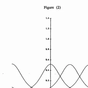
180 -150 -120 -90 -60 -30 0 30 60 90 120 150 180
Figure (1)
1.0 • •
0.6
0.2
180 -150 -120 -90 -60 -30 0 30 60 90 120 ISO 180
Density of the von Mises distribution for k = 2 and [Xq = 0, 90, 180.
1.4 T
8
0.4
0.2
-180 -ISO -120 -90 -60 -30 0 30 60 90 120 150 180
[image:19.621.92.447.67.421.2]i
10
2.2 Sim ulation of the von M ises D istribution
We use the algorithm described by Best and Fisher(1979) to simulate samples from the von Mises distribution with mean equal
to zero and k specified. The steps of the algorithm are as follows :
1. Take uj , U2 and U3 to be pseudo random observations from U(0,1). New observations uj , U2 and U3 are used each time steps 5-8 or 10 are executed. Methods for generating these pseudo random observations are discussed in section 2.3.
2. set X = 1 + ( 1 + 4 ,
3. set p = ( X - ( 2x ) / 2k ,
4. set r = ( 1 -f p2 ) / 2p ,
5. set z = c os(tcuj) ,
6. set f = ( l + r z ) / ( r + z ) ,
7. set c = K ( r - f ) ,
8. if c ( 2 - c ) - U2 > 0 go to step 10 .
9. if In ( c / U2 ) + 1 -
c
< 0 return to step 5 .10. set 0 = [ sign ( U3 - 0.5 ) ] cos'^( f ) .
To generate samples with a mean p not equal to zero we need the following step :
This algorithm is based on using the wrapped Cauchy distribution and henceforth will be called the wrapped Cauchy method. Best and Fisher compared this method with ones described by Mardia(1972), Siegerstetter(1974) and one using a polynomial envelope. They showed that their method is superior to either Siegerstetter's or the polynomial envelope method , in terms of timings although the latter is reasonable for small k. They also
showed that Mardia’s method based on the wrapped normal distribution is good for the extreme cases as k -> 0 and jc -> oo but
not for intermediate values of k. Siegerstetter's method also has
the disadvantage of being costly to use on the computer. Finally they showed that the wrapped Cauchy method was simple to program and fast for all values of k and consequently can be
considered more efficient than the other methods.
12
2.3 Random Numbers and Randomness
We have two methods for generating pseudo-random
observations from U(0,1). The first method is given by subroutine
[ G05CAF ] of the NAG library and the second method is described in a reference called "Guide for Fortran programming". The second method depends on setting a value for the argument (seed) which is updated automatically. It is recommended that the value of the seed be chosen to be a large odd integer.
We initially chose two different values of the seed namely 99 and 99999. Each value of the seed produces a different set of random observations.
Using the two seeds and the NAG subroutine gave three different ways of generating random observations from U(0,1). In order to choose which method of the three to use , we carried out the following procedure:
1. Using each method, we generated a random sample of size 4(X)0.
2. For each sample we did a Runs test for randomness using the package MINITAB.
3. The results obtained are as follows :
When using the method from the NAG Library we have : -
The observed number of Runs = 2031.
The expected number of Runs = 2000.9995
The test is significant at a = 0.3429 and so we cannot reject randomness at the 5% level.
When using the second method with seed = 99 we have :
The observed number of Runs = 2000
The expected number of Runs = 2000.0754
1957 observations above 0.5 and 2043 below.
The test is significant at a = 0.9981 and so we cannot reject randomness at the 5% level.
When using the second method with seed = 99999 we have :
The observed number of Runs = 2008
The expected number of Runs = 2000.9955
2003 observations above 0.5 and 1997 below.
The test is significant at a = 0.8247 and so we cannot reject randomness at the 5% level.
■
14
2.4 The Chi-squared goodness of fit test for the von Mises
distribution
We use the Chi-squared goodness of fit test to test whether the simulated samples adequately fit a von Mises distribution. In order to apply the Chi-squared test we must subdivide the circle into a number of arcs i.e. group the data into suitable angular intervals. In each arc we count the frequency of sample points and
calculate the expected frequency from Appendix 2.1 of
Mardia(1972) or Table E of Batschelet(1981). The fit of the distribution is considered to be satisfactory if the observed frequencies do not deviate too much from the expected frequencies. The angular intervals need not be equally spaced , but the expected frequency in each interval must not be too small and preferably at least five.
The Chi-squared test statistic is as follows :
k
X —
1=1
where k is the number of intervals , Oj the observed frequency and Cj the expected frequency in the ith group. This statistic is approximately distributed as a % random variable with k -1 degrees of freedom.
We now give some examples of testing the fit of simulated data to the von Mises distribution. We test whether the fit is good at a significance level of a = 0.05.
No of
ob serv a tio n The valueof K
No of group
in te r v a ls 5% critical value;tables Conclusion
Example 1 200 0.4 18 12.0774 27.59 accept fit
Example 2 500 0.4 18 21,0.03 27.59
Example I 200 1.0 12 4.75345 19.68
Example ^ 500 1.0 12 11.1378 19.68
Example 5 200 4.0 8 6.94747 14.07
Example i 500 4.0 9 9.29443 15.51
16
2.5 Mixtures of von Mises Distributions
The probability density function of a mixture of two von Mises distributions is given by :
f ( 0 ) = p f i ( 0 ) + ( l - p ) f 2 ( 0 ) O <p < 1 , O < 0 ^ 2tc
(2.4)
where
fj(0) = [2n Io(Ki))“^ exp{Kj cos(0 ~ pp)) i = 1,2, kj > 0 , 0 ^ pj < 27c,
is the von Mises pdf discussed in Section(2.1). p is the mixing parameter. We refer to (2.4) as the five parameter mixture distribution. The special case where Kj = K2 and P 2 = P i + 7C is referred to as the three parameter mixture distribution.
Model (2.4) was first suggested by Gumbel(1954) in connection with various sets of data, however, he did not use the model because of the analytic difficulties involved.
Mardia(1972 pp. 128-130) discussed the analytic difficulties and obtained estimates of the parameters by using the method of moments .
Stephens(1969) also suggested using (2.4) with kj = K2 and the two modes 180° apart i.e.
f(0) = {2n Io(k)}'^ [ p exp{ k cos(0-p) } + (1 - p ) exp{ -k cos(0-p) } ]
(2.5)
although, when fitting to data he used the simpler version of (2.5) with p = Y i'G.
f(0) = [2n Iq(k)}"^ cosh ( k c os(0 - p ) ) (2.6)
This method was extended by Spurr(1981) for bimodal data on the range( 0, tc ).
18
May estimates are : p = 0.803, k = 3.167, p = 61.5,
Stephens estimates are : p = 0.803, k = 3.05, p = 63.08 and
Mardia estimates are : p = 0.78, k = 3.553, p = 61.4 .
40 ^
36
32
-28
-24
-20
16 . .
12
8
-4
-40 80 120 160 200 240 280 320 3601
Figure (3)
20
2.6 Simulation of Mixtures of von Mises Distributions
To simulate random samples of size n from a mixture of von Mises distributions we do the following :
-1. We simulate n observations from each of g(6 ; , %%) and
g(0 ; P2 , K2> using the previous algorithm of Best & Fisher(1979).
2. We choose the required value of the mixing parameter , p.
3. We generate n random numbers from U(0,1) , say , ul, u2,
,un.
4. Finally we create a sample of n observations from the specified mixture distribution by applying the following procedure :
-(i) If ul < p then the first observation from the simulated
----g(0 ; Pi , Kj) will be taken into the mixture and if ul > p then the first
1
observation from the simulated g(0 ; P2 , K2> will be taken into the mixture.
(ii) We repeat this process using the remaining random numbers u2 , u3 , ... , un to obtain the required sample from the mixture distribution.
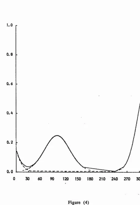
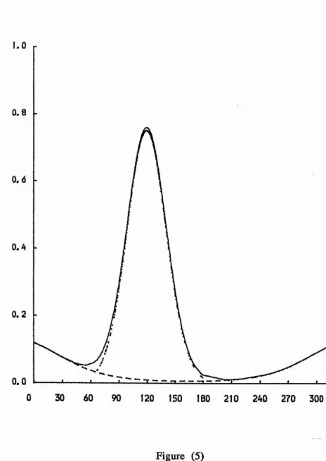
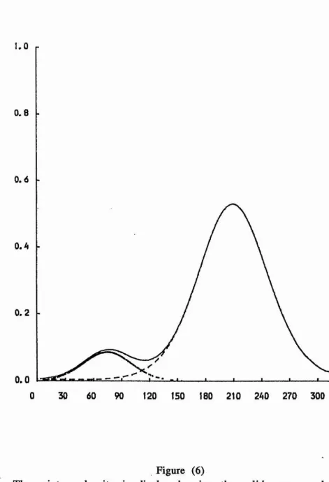
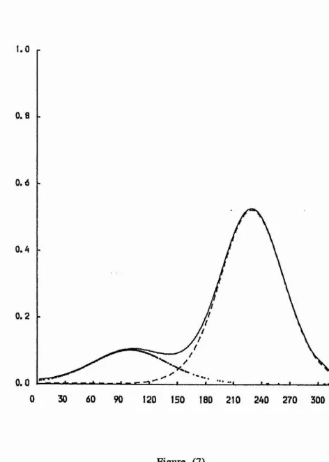
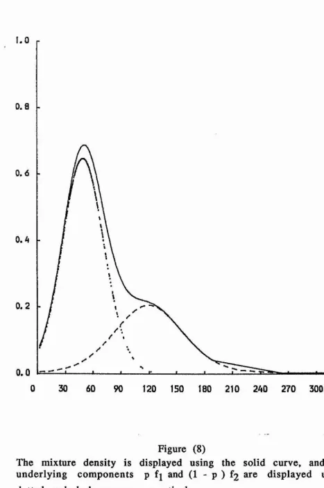
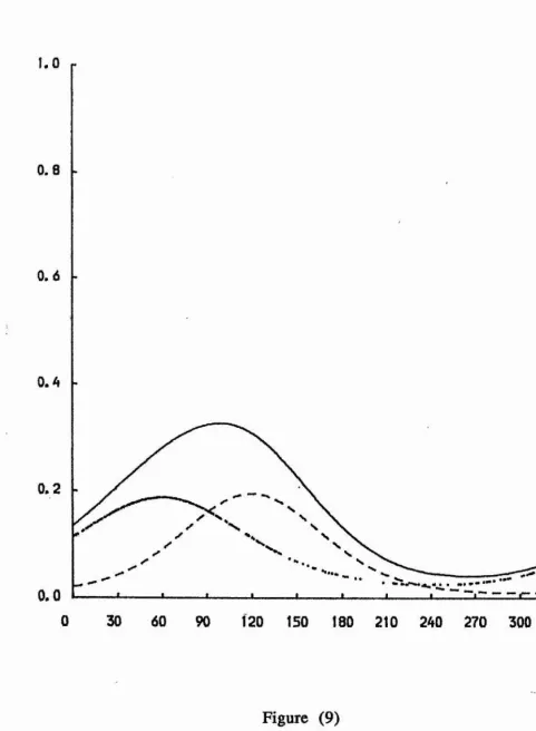
Figures (4) - (9) illustrate the mixture of two von Mises
densities for the six examples discussed in Section (4). Also, the
figures show the underlying components p fj and (1 - p) f2*
1 . 0 r
0.8 .
0.6
0.4
0.2
0.0
120 150 180 210 240 270 300 330 36C
Figure (4)
The mixture density is displayed using the solid curve, and the
underlying components p f\ and (1 - p ) f2 displayed using
dotted and dash curves, respectively.
[image:32.612.63.522.46.714.2]1.0
0.8
.
0,6
0.4
0.2
0.0
30 60 90 120 ISO 180 210 240 270 300 330 360
Figure (5)
The mixture density is displayed using the solid curve, and the underlying components p fj and (1 - p ) f2 are displayed using dotted and dash curves, respectively.
[image:33.615.64.528.62.717.2]24
1.0
0.8
0.6
0.4
0.2
0.0 JdL
3
30 60 90 120 ISO 180 210 240 270 300 330 360 0
Figure (6)
The mixture density is displayed using the solid curve, and the underlying components p fj and (1 - p ) f2 are displayed using dotted and dash curves, respectively.
[image:34.613.61.533.60.750.2]1 . 0
0.8
0.6
0.4
0.2
0.0
0 30 60 90 120 150 180 210 240 270 300 330 360:
Figure (7)
The mixture density is displayed using the solid curve, and the underlying components p fj and (1 - p ) f2 are displayed using dotted and dash curves, respectively.
[image:35.612.56.528.57.719.2]26
Î.O
0.8
0.6
0.4
0.2
0.0
30 60 90
0 120 150 180 210 240 270 300 330 360
Figure (8)
The mixture density is displayed using the solid curve, and the
underlying components p f\ and (1 - p ) f2 are displayed using
dotted and dash curves, respectively.
[image:36.612.58.525.69.771.2]Î.O
0.8
0.6
-0.4
0,2
0.0
30 60 90 120 150 180 210 240 270 300 330 360
Figure (9)
The mixture density is displayed using the solid curve, and the
underlying components p fj and (1 - p ) are displayed using
dotted and dash curves, respectively.
[image:37.615.45.527.74.730.2]28
C
HAPTERS
METHODS OF ESTIMATION
3.1 Maximum Likelihood Estimation
In this section we introduce the maximum likelihood method for estimating the parameters of statistical distributions.
Let xj , X2 , ... x^ be independent observations from a density say , f( x ; a ) , where a is the parameter vector we wish to
estimate. The likelihood function is defined by
L( a ) = n f(xj ; a ) . (3.1)
j= l ^
It measures the relative likelihood that different a will have given
rise to the observed x's .
The maximum likelihood method finds the particular a say, a q
which maximizes L , i.e the a q such that the observed x s are
more likely to have come from f(x ; a q) than f(x ; a ) for any other value of a.
It is usually more convenient in practice to maximize
n
X(a) = L oggL (a)= J ^ L o g e f ( x j ; a ) (3.2)
j= l
For many parameter estimation problems one can tackle this maximization in the traditional way of differentiating X(a) with respect to the components of a and equating the derivatives to zero to give the normal equations
dX
3 ^ = 0 (3 3 )
These are then solved for the a j and the second order derivatives are examined to verify that it is indeed a maximum which has been achieved and not some other stationary point.
For simple parametric models the maximum likelihood approach is very popular , partly because of the existence of attractive asymptotic theory , and partly because the estimates are often easy to compute.
For mixture distributions , however , the normal equations are not usually explicitly solvable and so iterative techniques have to be adopted.
The problem of obtaining the maximum likelihood estimates of the unknown parameters in the mixture of two linear normal distributions has been extensively studied in the literature by , amongst others , Hasselblad(1966) , Day(1969) , Wolfe(1970) ,
Hosmer(1973) and Fowlkes(1979). For further details see
Titterington et al (1985).
30
and Dempster, Laird and Rubin(1977) - the EM algorithm ). The EM
(Expectation - Maximization) algorithm given by Dempster , Laird and Rubin(1977) has become very popular recently and has been applied to many problems in statistics. Its main drawback is the slowness of convergence ( see Everitt & Hand 1981 ) but this is compensated for by its simplicity and other properties. For further discussion and more details see Titterington et al (1985).
Unfortunately , whenever the two variance terms cannot be assumed equal , iterative numerical techniques may break down in practice ( see Quandt and Ramsey(1978) ).
For the mixture of two von Mises distributions the likelihood function is also unbounded and so iterative techniques are again necessary. Jones and James(1969) used a procedure formed from a combination of the gradient method and Newton - Raphson method. We use a modified Newton algorithm which is available as subroutine (E04JAF) of the NAG library.
3.2 MOMENT ESTIMATION
Karl Pearson(1894) first used the method of moments to estimate the parameters in a mixture of two linear normal distributions. However , there are two major problems to overcome when the method of moments is applied to the mixture of two linear normal distributions. Firstly, we need to solve a high order polynomial equation and secondly , multiple solutions may exist. For an extensive bibliography and further details see Titterington
et al (1985) and Everitt and Hand(1981).
We can adapt the method for the mixture of two von Mises distributions and make use of the sine and cosine moments . However , as noted by Mardia(1972) , there is the problem of selecting an appropriate set of trigonometric moments to estimate the five unknown parameters. When the first two sine and cosine moments are used there is no symmetrical way of constructing the fifth equation. For the special case when kj = K2 and m^2 M^l + ^ i.e. the three parameter case, Mardia(1972 pp. 128 - 129) described a way of obtaining estimates of the parameters using the method of moments. Spurr(1981) extended this method for data which are bimodal on the range (0 , k) .
32
P
The five moment equations are then
— cos(t m ) + (1 - p ) — cos(t H2) = - ^ c o s ( t 0i)
(3.4)
P m ) + (1 - P > i3 0 ^ ünO P2) = n ®i) ’
for t =1,2,
and
{2^l0(K ^)}'^cxp{K |Cos(epP|)) - {27clo(K2)}'^exp{K2COs(9|"P2) 1
y
Jbmm4 P{2tcIo(kj)} ^exp{KjCOs(0j-Pi)} + (l-p){27cIo(K2)}'^exp{K2COs(0i-p2)}
= 0 (3.5)
Another method which is considerably quicker with regard to
CPU time can be obtained by using the first three sine and cosine
moments i.e. the six equations obtained from (3.4) with t = 1, 2, 3.
34
3.3 MINIMUM DISTANCE ESTIMATION
Minimum distance estimation was first introduced by Wolfowitz(1957) and the methods are usually based on distribution functions or transforms of the distribution function. Although less efficient than maximum likelihood when the assumed model is correct this method of estimation is more robust against heavy - tailed departures from the model ( see Woodward et al (1984) ).
Also , Parr and Schucany(1980) showed that minimum distance
techniques can provide robust estimators of the location parameter of a symmetric distribution.
The methods proposed so far in the literature fall into two main categories :
(i) measures based on the distance between the empirical and theoretical distribution functions ;
(ii) measures based on the distance between some transforms of the empirical and theoretical distribution functions.
normal but minimum distance gave better estimates under symmetric departures from normality.
Under (ii) , Quandt and Ramsey(1978) used a measure based on the squared distance between the empirical and theoretical
moment generating functions. Heathcote(1977) introduced a
measure based on the integrated squared error between the empirical and theoretical characteristic functions. For further details see Titterington et al (1985).
Methods of estimation based on the characteristic function are particularly useful for the mixture of two von Mises distributions since the characteristic function can be obtained in an analytic form and is always bounded. We also use a Cramer-von Mises type measure for comparative purposes but find that this is much slower and does not give estimates which are substantially better.
36
(i) The Cramer-von Mises measure
This measure minimises n
(3.6) i=l
w here
8i
F(8i) = p
J
{2tcIo(ki)}’^ exp{Kicos(x - p^)) dx0
(3.7)
8i
+
(1 - P)J
{27cIo(x2))”^ exp{K2Cos(x-
P2))0
and 0j[ is the ith order statistic of the sample. Calculation of F(0j) is slow and considerably increases CPU time.
(ii) The characteristic function measure
The use of the characteristic function as the particular form of the transform has been discussed by , among others , Paulson , Holcomb , and Leitch(1975) , Bryant and Paulson(1979) ,
Feuerverger and McDunnough(1981) and Heathcote(1977). Since
the characteristic function is always bounded and can be expressed in a closed form , we introduce a method based on the characteristic function for estimating the unknown parameters in a mixture of two von Mises distributions.
The characteristic function measure minimises
X
I |2l® n(t) - ® (t) I t=l
w here (3 .8)
1 ^
^ n (0 = ÎT 2 ,^xp(it8j)
j= l
is the empirical characteristic function ( ecf) of the sample Gj ,02 , 0JJ , and 0 (t) is the characteristic function of the model.
To find the characteristic function of (2.4) we must evaluate
38
Now
2k
E( cos 0t ) = Jcos(0t) f(0) d0
0
2jc
= p {27C Jcos(0t) CXp{KjCOS(0 - \Li)] d0
0
2k
J
+ (1 -p) {2tc Io(k2)}"^ Jcos(0t) exp{K2COs( 0 - P2)}
If we put z = 0 - pj , dz = d0 we get
2k 2k
j^cos(0t) e x p { K j c o s ( 0 - p i ) } d 0 = f c o s { ( z + p j ) t } e x p ( K j c o s z ) d z
0 0
27t
= J(cos z t COS P | t - sin z t sin p j t ) e x p ( K | C O s z ) d z
0
231
= COS pjt Jcos (zt) exp(Kjcos z )) d z
0
2k
0
= 23C COS (pjt) Ij(Kj) .
2îï
j
0
Since
Jcos
(zt) exp(Kjcosz) dz = 2n Ij(K][) andJsin zt exp(KiCos z) dz = 0 , for t = 1,2,.
2ic
J
0
( see Mardia (1972, p .62 ) ) .
The function I^(k) is the modified Bessel function of the first kind and of order t .
Therefore
Ij(k2>
E( COS et ) = p cos(t + (1 - P ) cos(t P2>
Similarly we have
2tc
E( sin 0t ) = Jsin(0t) f(0) d0
0
23C
= p {2tcIo(kj)}‘^J*sin(0t) exp{Kicos(0 - p^)} d0
23C
w ith
2n 2n
f s i n (0t) c x p {K i co s (0- p i ) ) d0 = f s i n { ( z + p j ) t ) e x p ( x ^ c o s z ) d z
0 0
271
= J(sin
z t c o s p j t + c o s z tsin
p j t ) e x p (K ] ^ co s z ) d z0
27t
= COS p j t
Jsin
z t e x p (K j co s z ) d z0
2tc
+ sin p j t Jcos z t exp(Kjcos z ) d z
0
2% sin p^t I j( k i )
Therefore
I ( k 2)
E( sin 0 t) = p sin(t p^) + (1 - P ) sin(t P2)
Hence the characteristic function of (2.4) is given by
40
' %
I
0 (t) = p { cos(t P j ) + i sin(t pj)}
lO(Ki)
+ (1 - p ) { co s(t P2) + i sin (t P2>} V ^ 2)
Paulson , Holcomb & Leitch(1975) developed a numerical method for estimating the parameters of the stable law by minimizing the integral
2 -t2
( t ) - 0 ( t ) | e " dt (3.10)
They found that this estimation procedure worked well for some parameter values but failed to give reasonable results for other parameter values.
This method was generalised by Heathcote(1977). He introduced a measure based on the integrated squared error between the empirical and theoretical characteristic functions for estimating the parameters in a mixture of two -linear normal distributions. Heathcote investigated the properties of the statistic 0jj which minimizes
In(®)= J l l> n ( t ) - « * ( t , 0 ) l ^ dG ( t ) (3.11)
-oo
where O (t,0) is the theoretical characteristic function and G(t) is a nondecreasing weight function whose total variation can be taken
as unity. The choice of weight function G(t) is very important with
regard to the efficiency of the estimator and convergence of the method.
42
the variance of a normal distribution centred at the origin , then reasonable efficiency is achieved if the weight function assigns most weight to an interval about the origin. There may also be circumstances where it is preferable to minimize
|2
Æ l* n
at one , or only a few values of t rather than using a weight function distributed over the real line. He compared the integrated squared error estimate with the maximum likelihood estimate based on random samples of size n from a N(O,0) distribution using
.2
the weight function G(t) = e .H e found that maximum likelihood gave better results when the sample size was 25. When the sample sizes were 50 and 100 the results obtained from both methods were very similar. He also used the same weight function in the calculation of the integrated squared error estimate for the example of Cox & Hinkley(1974 , p . 291) for which the density is given by
For this example Heathcote found that the maximum likelihood estimator was inconsistent but the integrated squared error estimator was consistent.
Heathcote’s method depends on the choice of t and weight function G(t) while this is less important for our method.
In order to minimise (3.8) we note that (3.9) involves Bessel functions of order t and these decay as t increases (see Kent 1977). Consequently we may not need to include too many terms in the summation for convergence to be achieved.
Equation (3.8) was minimised when the number of terms in the summation was taken as 2 , 5 , 8 and 10 respectively. The convergence when using 5 , 8 and 10 terms was satisfactory although CPU time increases as the number of terms increases. When only two terms are taken in the summation we find that the convergence is unstable , in other words when we use different initial values to start the minimisation procedure we get different final results. Hence we shall only consider using 5 , 8 and 10 terms in the summation.
44
An alternative expression for (3.8) can be obtained by substituting (3.9) into (3.8) , expanding the square , and making use of the von Neumann addition formula which is given by
Io{(
Ki^ + K;Z +2
kjK
2
co se
= Io(
Ki)
Iq(
K
2
)
+ 2^Ij(K j)Ij(K 2)coset (3.12)
t= l
This leads to
I i2 I 1
|4>n(t) - 0 (t) I = I “ ^ ex p (itej) - p { cos(t p j) + i sin(t pj)} j= l
I/K 2) |2
(1 - p ) { cos(t P2> + i sin(t P2>} ,
I
I r
1
^
rI^^l)
1
/^
2
)
n= IL - ^ c o s(te j) - { p cos(t + (1 - P ) cosCt P2) }]
. r l ^ f ^((*^1) n |2
+ 1 1 - {P S‘“(‘ ' P ) P2) }] I
r 1 ^ f ^((^2) n 2
= L n 2 (^os(t8j) - {p cos(t a P) cos(t ^2) î ^ ) ]
+ g - {P &W P l % [ ) + (1 - p ) s m ( tH 2) ^ g ^ } ]
= [ C - ( a i + a 2 ) ] + [ S - ( a, + ) ]
w here
n
- 1 ^
C = - ^ c o s(t0j) . ai = p cos(t ,
- 1 ^
a2= (1 - p ) cos(t P2) . S = - ^ s in (t6j)
j= l
. , Ij(k2)
aj = p sin(t and a^ = (1 - p ) sin(t P2> Hence lo„(t) - 0 (t) | = C 2C ( a^+a^ ) + ( a^+a^ )^ + S ^
- 2 S ( a^+a^) + ( a;+a^ Ÿ
“ C ^ + S ^ - 2 ( C (a^+a^) + S (a^+a^) ) + (aj+a2)^ + (a^+a^)^
Now (aj+aj)^ = a^^ + a^^ + 2 a^a^ = p2 cos2(t P i)[ ~ ^ ] ^
. 1 rV * 2) i 2
+ (1 - p )2 cos2(t P2>
It(Ki) I.(K2) + 2 p (1 - p)cos(t Pi)cos(t P2)ro (-)ïo (K 2)
46
(83+84)^ = 8)^ + 84^ + 203 34 =
+ (1 - p )2 sin2(t p2) [ ^ f
L (ki) L(K2> + 2 p ( l - p) s i n( t pi ) s i n( t p2) ï 3^ i ^
Therefore
(31+32)2 + ( 3 3 + 3 4 ) 2 = p 2 [ ^ ] \ ( 1 - p ) 2
I,(Ki) I (K2) + 2 p ( l - p ) co s t ( m - p 2 ) io(Ki)Io(K2)
consider now
C (a^+&2) —
1 ^ f
- ^ c o s(te j) (p cos(t (1 - P ) cos(t P 2 ) ^ ^
j= l
S(ag+a^) =
- X « n (te j) {P sin(t m ) ^ ^ + (1 - P ) Sin(t P2> }
I.(Kl) 1 ^
Then C(aj+aj) + S (33+34) = p . - ^ c o s t(0j - p j)
j= l
I((K2) 1 A
C^ + S ^ = { ^ ^cos(tej) } ^ + {^ ^ sin (te j) } Rj say .
j= l j= l
Collecting these together we have
oo
^ I C - (a i + a j) + i ( S - (aj + a^)) P
t= l
eo
S J 2p " V T
t= l
X p> X " * ’* ' ( ^ 1 - ^ 2 ) ^ ' ê è
t=i t=i
Using (3.12) we then have
oo
% y K i ) y K 2 ) COS t(P i - P2) = t= l
J % (( + «2^ + 2kjK2 cos (Hi - P2> - JIqCki) lo (f2 )
48
Therefore
Z . “ ’ k w
t=l
r Io((Ki2 + K2^ + 2kiK2 cos(m - P2))^^^}
P(l- P> L lo(Ki) Iq(k2) - I J
and
X
Io(K2)-‘ [I0(k2)]2 2'- ^ 0'^ ""2' + «2^ + 2x22)1/2 } . i ( I0(X2) }2]t=l
( von Neumann formula with = |i2 ) »
oo
Also ^ ® = Io(z) + 2 ^ Ijj,(z) cos (me)
m =l
( see Abramowitz & Stegun p . 376 )
Therefore
oo
XT' 1 1
2 _,It(^) cos t(6j - P i ) = j exp(z cos(6j - pj)) - JIq /^ )
W hence
^ | o „ ( t ) - 0 (t) P= ^ - n i ^K i )S ® ’‘P f ’' I cos(ej - P i ) }
(1-p)
J=1
^ (l-p)2 Io(2k2> ^ + «2^ + 2k iK2 cos(pi-p2))l/^) ^
2 w g ? ' « - " - I ---w i ^ ) w « 2)---'
+ 2 (3.13)
The first and last terms on the right hand side of (3.13) do not depend on the parameters to be estimated and so can be omitted from the optimisation routine. All the Bessel functions have been reduced to order zero and no longer depend on t. Hence we no longer have an infinite sum in t to contend with.
We use a standard subroutine (S18AEF) of the NAG library to calculate the Bessel function Iq. There is an overflow problem with
the Bessel function when the argument is greater than 80 and this is caused by either k j or K2 becoming very large in the iterative optimisation procedure. Setting upper bounds for the k’s prevents
an overflow but in practice one of the k's reaches the limit. This can
happen for any initial values . One way round this difficulty is to use the following large k approximation to Iq
exp(Kj) 1
50
This gives
iQ(2Ki) 1 1 2,x ;
i w F . 1 . j _ , 2
1 8kj 1
2 (3.15)
Io((Kl^+ + 2kiK2 cos(pi - P2»^^^)
Io(ki)Io(k2)
using (3,14) we have the following .
If S = {kj^2+ K2^ + 2kjK2 cos(pj[ - ^ 2)) is big then either kj and K2
are big and so
Io(S) exp(S-Ki-K2)(2juKi)l/^(2jtK2)l/^{l )
Io(>'l) lo(K2) (2xS )1/2 { 1 + ^ ) ( 1 + ^ )
or Kj is big and K2 is small and so
%o(S) e x p (S -K i)(2 n x i)l/^ {l + ^ } j
io(^l) ^0(^2) (2jcS)^^^{l + } ^0(^2)
8k^
[The term 19(^2) can then be calculated by using the NAG Library
subroutine .]
or «2 is big and kj is small and so
Io(S) exp(S-X2)(2xK 2)l/^{l + ^ ) j
io(^l) ^0(^2) (2jcS)^^^{1 + —-—) io(^l)
In which case Io(>^l) can be calculated by using the NAG Library subroutine.
Finally we can write n
j^ X e x p { K iC o s ( 0. - Pi)) =
j ~ l
> exp[-Ki{l-cos(0 . -
Pi)}]---;---for large K| ( i = 1, 2 ) .
Using this approximation for Iq improves the convergence but
it does not work for all samples and so we still have samples where
one of the k's reaches the upper limit. This seriously affects the bias
52
C
HAPTER 4
DISCUSSION OF RESULTS
In this chapter we demonstrate our results with two kinds of data ;
( 1 ) Simulated data.
( 2 ) Real data introduced in Section(4.2).
The minimisation subroutines require initial values i.e. starting values for the five parameters Pi , P2 » ^1 » ^2
P-Mardia(1972) gave an explicit method for estimating the
parameters p , k and p for the three parameter model (2,5). Our
starting value procedure uses this method to obtain estimates of p ,
Ki and p j. We then set K2 = k j and P2 = P i + w to obtain starting values for K2 and
P2-The procedure is as follows
(1) estimate p i from the equation
n n
tan(2pi)-= ^ s in ( 2 e i) / ^cos(20j|) (4.1)
i=l i=l
where Gj ,6 2 » ...» the observed angles ;
(2) estimate ki from the equation
1 ^ 1 n
(2p - 1) A (ki) = c o s (P i ) - X c o s ( e i ) + sin ( P i ) ~ ^ s i n ( e j )
i = l i = l
(4.3)
Il(K l)
where A {ki) = — . Values of A (k j) are tabulated in Appendix
2.2 of Mardia(1972) and also in Table 3 of Spurr(1981). For large Kj
1 ^1 ^1^
we have A(x^) = 1 - , and for small k j , A (k j) = y - yg* (see
Appendix 1 of Mardia(1972)).
Equation (4.2) is difficult to invert for although selected values are given in Table 3 of Spurr(1981). However, since
l2(^l) , A (k i)
_ - _ 1 - 2 { --- } then we can make use of the aboveIqVKj; Kj approximations to A (k j),
For large kj equation (4.2) becomes
I.e.
2
Kj 5 . (4.4)
( 1 - &2 )
For small kj equation (4.2) becomes
54
I.e.
Kl = ( 8 R2 )1/^ . (4.5)
We suggest using approximation (4.4) for values of R2 > 0.5
and approximation (4.5) for R2 < 0.5.
4.1 The Simulated data:
We have two ways of comparing the results for the different methods of estimation discussed earlier.
(i) The first way is to compare the results for single samples of different sizes i.e. n = 50,100 and 200. The reason for doing this is , firstly, to see how close the estimates of the unknown parameters get to the true values and, secondly, to see how much CPU time is
taken. However, because of sampling variations we would need to
look at many samples to get an overall view of the relative performances of the various methods.
(ii) The second way is to generate many samples of the same size
and compare the bias and MSE for the different methods. This way
will give us a better overall idea of the relative merits of the different methods.
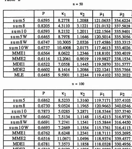
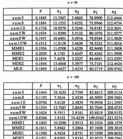
We represent maximum likelihood estimation by MLE, moment estimation using five equations by M M El, moment estimation using six equations by MME2, minimum distance estimation based on the Cramer-von Mises measure by MDEl and minimum distance estimation based on the simplified characteristic function measure (3.13) by MDE2, Minimum distance estimation when using 5, 8 and 10 terms in the summation (3.8) without a weight function will be denoted by sum5, sum8 and sum 10 and with a weight function by sum5W, sum8W and sumlOW.
56
Tables 1 - 6 display the results for the six simulated data sets which we shall use throughout this section. These are :
Example 1: p= 0.35,ki = 3.5,K2 = 6.0, 100, P2= 320
Example 2: p = 0.70,kj = 7.5,K2 = 1.5, 120, p2= 340
Example 3: p = 0.10,ki = 5.0,K2 = 2.5, 75, p2= ^10
Example 4: p = 0.20,K^ = 2.0,K2 = 3.0, p^= 100, P2= ^30
Example 5: p = 0.65,Ki = 6.5, %2 = 2.5, p%= 50, P2= 120
Example 6: p = 0.55,kj = 1.0, K2 = 1.5, p^= 60, P2~ 120.
These simulations were generated using the method described in Section(2,6).
Each method of estimation discussed in Chapter 3 was implemented for the above mixtures.
We compared the final results obtained firstly when the true values were used as initial values and secondly when the initial values were obtained from the procedure described at the beginning of this chapter.
In practice, of course, we will never know the true values but the purpose here is to show that the final results do not depend on the initial values used.
A A
If either | p(Tru) - p(ini) 1 < 0.01
(4.6)
A A
A
p(Tru) is the estimate of p when the true values are used as
A
initial values ,p(ini) is the estimate of p when the initial values are obtained from (4.1) - (4.3), then we consider the two results to be in good agreement.
We need both conditions in (4.6) since sometimes p and (1-p) are interchanged in the final results with consequent changes to the other parameters.
Generally, the estimates of p j and P2 are close to the true values (see tables 1,2,3,5) although there is some variability
between the different methods of estimation. In table 4 some of the
methods give values of p j which are very different from the true
values although they get closer as j i increases. We have problems
with example 6 (see table 6) since most of the parameter estimates
are not close to the true values. This is to be expected since the
mean directions are close together, the concentration parameters are almost equal and small and as shown in figure (9) the distribution is unimodal.
The estimates of k\ and are very variable, often one of
them will be reasonably close to the true value but the other will generally be much bigger. Usually they get closer as the sample size
increases but not always. There are big differences between the
58
The estimates of p also vary considerably from method to method. Again, as n increases the estimates generally get closer to the true values. As we might expect the estimates of p are better when the concentrations are large and the modes are separated.
From these tables, it does not seem that one method produces consistently better results than any of the others. However, in most
cases the CPU time taken when using MME2 and sum5W are similar
and these methods are the fastest over all. Also, MMEl and MDEl take a large amount of CPU time and do not give substantially better estimates than the other methods. Consequently we decided not to include them in the bias and MSE comparisons.
Increasing the sample size usually improves the accuracy. Also, the use of the weight function does not consistently improve the results.
Secondly, we consider some comparative measures based on sets of samples namely the bias and MSE. We simulated 50 and 200 samples of size 50 , 100, 200 for each of the six examples given earlier.
In order to compare the different methods of estimation discussed earlier the bias and MSE for each parameter were calculated for each set of samples. Samples which did not satisfy condition (4,6) were noted but excluded from the bias and MSE calculations. Samples where one of the k's reached the upper limit
were also excluded.
which compares sum5, sum8 and sumlO with sum5W, sumSW and sum low to find out which seems to be the best. Also included are the results for MME2, MDE2 and MLE for comparison with this best method.
Each table gives the bias and MSE for each of the parameters and indicates the number of samples satisfying condition (4.6), Cl, and the number of samples which converge but do not satisfy condition (4.6), 02. The number of samples where one of the k's
reaches the upper limit is denoted by 03.
It is clear from tables 7-12 of example 1 and tables 13-18 of example 2 that the use of the weight function reduces the bias and MSE for all the parameters. In addition the number satisfying condition (4.6) is increased. There is little difference between sumSW and sumlOW as far as bias and MSE are concerned but sum5W generally does better in this respect. All the samples converged when sum5W , sumSW and sumlOW were used but condition (4.6) was not always satisfied. However, there is only one case where this condition is not satisfied by sum5W. Also, the average CPU time taken when using sum5W is less than that when using either sumSW or sumlOW. Consequently we choose sum5W as our best method. In other words we need take no more than 5 terms in the summation to ensure convergence and the smallest bias and MSE.
6 0
cases but is much better than MDE2. MLE always converged but did
not always satisfy condition (4.6) . Also, the average CPU time taken when using MLE is greater than that when using either sum5W or MME2 but is similar to that when using MDE2. Thus if reduced CPU time is our main criterion we may prefer to use MME2 or sumSW.
Tables 19-24 give the results for example 3. These tables show that using the weight function does not always reduce the bias or the MSE for both sum8 and sumlO but most of the bias and MSE are reduced for sum5. In addition the number of samples satisfying condition (4.6) is increased when the weight function is used. In most cases sum5W performs better than sum8W and sumlOW with regard to bias and MSE. The number of samples which satisfy condition (4.6) when using sumSW is always greater than that when using sumlOW and, apart from one case ( table 20 ), is always greater than or equal to that when using sum8W. Also, the average CPU time taken when using sumSW is less than that when using either sum8W or sumlOW. Consequently we again choose sumSW as our best method. The tables also show that MLE performs better than MME2 , sum5W and MDE2 in almost all cases. MLE always converged but did not always satisfy condition (4.6). Also , MLE gave a greater number of samples satisfying condition (4.6) than MME2 , MDE2 for all cases but in some cases sumSW did better. However , the average CPU time taken when using MLE is greater than that taken when using either sumSW or MME2 but is similar to that taken when using MDE2.
and 28 show that using the weight function does not always reduce the bias or the MSE for some of the parameters. In fact the results are very variable , sometimes the bias is reduced and MSE increased or vice versa. In addition the number of samples satisfying condition (4.6) is increased when the weight function is used. In most of these tables it is clear that sumlOW performs slightly better than sum5W and sum8W as far as bias and MSE are concerned. However , the number of samples which satisfy condition (4.6) when using sum5W is greater than that when using either sumSW or sumlOW. Also, the CPU time taken when using sum5W is less than that when using either sum8W or sumlOW. For these reasons we choose sum5W as our best method.
The tables also show that in most cases there is little to choose between MME2 and MLE which in turn are better than sum5W and much better than MDE2. In many cases MME2 performs slightly better than MLE. Also, the average CPU time taken when using MLE is greater than that taken when using either sum5W or MME2 but is similar to that taken when using MDE2.
6 2
using sumSW is less than that when using either sumSW or
sumlOW we again choose sum5W to be our best method.
The tables also show that , in almost all cases , MME2
performs better than MLE , sumSW and much better than MDE2. Generally there is little to choose between MME2 , MLE and sumSW as far as the number of samples satisfying condition (4.6) is concerned. Clearly MDE2 does not perform as well as the other methods. The average CPU time taken when using MME2 is similar to that taken when using sumSW but is less than that when using any of the other methods.
Tables 37-42 show the results for example 6. In most cases the bias and MSE are reduced when the weight function is used. In addition the number of samples which satisfy condition (4.6) is increased. For this example , the average CPU time taken when using either sum 10 or sumlOW is excessive and the results do not seem to be substantially better than sum 5 or sum8 (see table 37). Consequently , we decided not to include either sumlO or sumlOW in the other tables for this example. From the tables it is clear that , in most cases, sum5W performs better than sum8W as far as bias and MSE are concerned. Also the number of samples satisfying condition (4.6) when using sumSW is greater in most cases than when using sum8W . Since the average CPU time taken when using sum5W is less than that when using sum8W we again choose sumSW as our best method.
condition (4.6) when using MLE is much greater than that when using MME2 , sumSW and MDE2. This will affect the bias and MSE calculations and may explain why MLE does not do well here. Also, the average CPU time taken when using MLE is greater than that when using either MME2 or sumSW but is similar to MDE2.
When the sample size n is increased the bias and MSE are reduced in almost every case for all the examples except example 1. For example 1 ( tables 7-12 ) , as sample size is increased the MSE is reduced in almost all cases but the bias seems to be very variable for some parameters. For examples 1- 5 the number of samples satisfying condition (4.6) is increased whilst the number where one of the k's reaches the limit is decreased. For example 6 there are
one or two cases where the number of samples satisfying condition (4.6) is decreased as n is increased. Increasing the number of samples S usually leads to a slight increase in the bias and MSE and also an increase in the number C2 of samples where one of the k's
reaches the upper limit. However, there is considerable variability both between and within the examples used. As noted earlier example 6 is very different to the other examples and this is shown by the results. There are also big differences between the magnitudes of the bias and MSE for the different parameters.
Table 1
50
64
P ^1 ^2 ^^1 P2 ZPU time (sec.]
sum5 0.3961 8.1523 5.5031 99.9763 317.5181 0.93
sum 8 0.37577 11.0286 5.0175 100.2130 317.3858 1.43
suml 0 0.3683 12.3763 4.9147 100.1888 317.3727 1.57
sum5w 0.3892 8.0791 4.9893 99.5977 316.7052 1.31
sumSw 0.3832 9.3283 4.7926 99.7806 316.7490 6.78
sumlOw 0.3822 9.5790 4.7688 99.7945 316.7590 7.25
MMEl 0.3836 7.3253 4.2423 99.2404 315.5838 15.03 MME2 0.3776 10.1019 4.3857 98.6314 316.6393 0.72
MDEl 0.3816 7.6267 4.7480 99.2662 315.9961 19.03 MDE2 0.3613 13.9269 4.8148 100.0927 317.3607 6.50
MLE 0.3825 7.7616 4.0803 98.4053 315.0984 7.10
n = 100
P Kl K2 -PU time (sec.]
sum5 0.3657 5.7891 6.1375 97.1296 318.0015 1.47 sum 8 0.4393 3.8136 10.8319 104.0203 324.3592 1.51 sumlO 0.4392 3.8158 10.8260 104.0199 324.3954 1.60 sum5 w 0.3620 2.8917 6.2417 98.2011 316.3398 1.06 sum 8w 0.3608 5.9576 5.8770 97,0198 317.7576 1.74 sumlOw 0.3606 5.9743 5.8680 97.0245 317.7603 2.03 MMEl 0.3564 6.3796 5.5090 96.9402 317.4967 28,04 MME2 0.3550 6.9591 5.5724 96.7238 317.8051 1.16
MDEl 0.3473 5.8736 5.3823 99.0807 318.0807 33.48 MDE2 0.3617 5.8163 5.8056 97.2668 317.9811 10.44 MLE 0.3558 6.6763 5.3424 96.3952 317.2158 10.97
n = 200
P Kl K2 M^l -PU time (sec.]
sum5 0.3941 4.0837 5.2387 98.9912 318,1771 1.22 sum 8 0.3934 4.0223 5.1496 99.1300 318.2298 1.27 sumlO ' 0.3933 4.0250 5.1448 99.1305 318.2311 1.29 sum5w 0.3021 3.3718 5.9261 103.5092 320.5620 0.94 sumSW 0.3621 3.6590 6.3785 98.4583 317.3888 1.66 sumlOW 0.3927 4.1836 5.2314 98.9571 317.9947 11.59
MMEl 0.3874 4.6963 5.1065 99.1952 318.0838 151.13 MME2 0.3905 4.4612 5.222 98.9616 317.8199 0.91
MDEl 0.3814 4,1707 4,8011 101.5129 318.8763 70.67 MDE2 0.3933 3.9974 5.1225 99.1362 318.2244 19.35 MLE 0.3873 4,7381 5.1033 99.1467 318.0392 20.78
[image:74.619.64.491.50.756.2]Kl K2 ^2 -PU time (sec.;
sum5 0.6595 8.2778 1.2088 121.0635 334.6224 1.13
sum 8 0.8205 4.3110 3.1221 121.0132 337.5828 2.1
sumlO 0.6593 8.2132 1.2011 122,1564 335.9401 6.41
sum5W 0.6465 8.7978 1.1646 120.5014 335.3056 1.29
sum 8W 0.6747 10.3005 2.0326 117.4586 333.3315 1.90
sumlOW 0.6737 10.4008 2.0173 117.4613 333.4026 2.13
MMEl 0.6564 8.0622 1.2346 118.8101 330.4019 18.45 MME2 0.6116 12.2061 0.9019 119.9827 338.1534 1.36
MDEl 0.6522 7.0558 1.1445 119.5870 331.5777 17.19 MDE2 0.6602 8.1414 1.2086 122.1241 335.7564 5.34
MLE 0.6485 9.5901 1.2244 119.4102 332.2022 6.13
n = 100
P Kl K2 H \^2 ZPU time (sec.]
sum5 0.6862 8.5233 1.3160 119.7171 337.4105 1.38 sum 8 0.6730 9.0524 1.1965 120.9663 340.0546 4.40 sumlO 0.7873 5.0285 3.2871 118.5344 337.3740 1.84 sum5W 0.6642 7.5134 1.1148 115.4213 316.9730 1.24 sum 8W 0.6691 7.2741 1.1541 115.3844 316.4450 1,60 sumlOW 0.6693 7.2669 1.1554 115.3761 316.4113 2.13 MMEl 0.6762 8.6248 1.2341 118.7111 335.2695 23,84 MME2 0.6516 11.0671 1.0496 118.9374 339.4577 1.24
MDEl 0.6781 7.3573 1.1858 118.0328 330.4956 35.25 MDE2 0.6719 9.0609 1.1895 121.0829 340.2594 10.86 MLE 0.6716 9.6885 1,1799 118.2027 333.6571 11.50
n = 200
P Kl K2 H % -PU time (sec.;
sum5 0,7309 6.7481 1.3079 118.6955 328.8135 1.01 sum 8 0.7337 6.6100 1.3243 119.4052 329.5861 1.93 sumlO 0.7342 6.5919 1.3281 119.4430 329.5655 6.97 sum5W 0.7209 7.0838 1.2973 118.4835 329.6974 1.08 sum 8W 0.7231 6.9491 1.3236 118.7764 330.1480 1.61 sumlOW 0.7234 6.9359 1.3261 118.7874 330.1453 2.11 MMEl 0.7278 6.9423 1.4228 117.6722 326.6865 43.80 MME2 0.6938 8.4420 1.0204 119.0877 333.2860 0.54
MDEl 0.7321 5.8988 1.3035 118.1735 327.0270 70.05 MDE2 0.7333 6.5815 1.3259 119.4561 329.5466 15.24 MLE 0.7273 7.5165 1.4871 117.9097 326.8847 15.70
[image:75.617.66.492.53.532.2]Table 3 66
n = 50
P Kl K2 ^2 -PU time (sec.;
sum5 0.1889 13.3567 3.4865 78.9900 212.4464 1.13
su m 8 0.1884 12.1553 3.4252 75.9966 212.4754 2.04
sumlO 0.1736 18.9579 3.3244 74.9187 212.3651 8.76
sum5W 0.1934 11.8390 3.5122 80.1076 211.5277 1.34
sum 8W 0.1937 10.6401 3.4916 78.9544 211.4829 1.94
sumlOW 0.1912 11.8128 3.4620 78.5222 211.4016 1.84
MMEl 0.1936 11.0708 3.6229 82.9600 211.3808 44.15 MME2 0.2020 8.1745 3.6247 82.4262 211,5900 1,21
MDEl 0.1834 7.4678 3.2227 84.6041 212.2295 16.87 MDE2 0.1846 13.6868 3.3977 75.7101 212.4426 5.65
MLE 0.1869 12.6427 3.4235 80.2719 209.9762 5.90
n = 100
P Kl K2 H ,H2 -PU time (sec.;
sum5 0.1444 19.1635 2.7789 83.8613 209.5114 1.54 su m 8 0.1193 7.5616 2.4530 65.5093 209.7601 2.33 sumlO 0.0796 5.6120 2.5839 79.9938 211.3593 8.69 sum5W 0.1554 13.7567 2.8643 83.7044 208.6753 1.54 sumSW 0.1624 9.1911 2.9181 83.8819 208.9152 1.86 sumlOW 0.8366 1.9152 74.4239 199.0342 221.5274 2.77 MMEl 0.1603 10.2290 2.9512 83.3524 208.1279 38.42 MME2 0.1811 5.8962 3.2004 87.7698 209.3019 1.03
MDEl 0.1580 6.5634 2.8751 87.3590 209.8632 33.13 MDE2 0.1571 9.8702 2.8333 82.9223 209.7561 10.53 MLE 0.1606 10.0409 2.9164 84.0177 208.1060 10.20
n s 200
P Kl K2 H 1^2 -PU time (sec.;
sum5 0.1059 14.3651 2.3216 80.5322 211.2128 1.52 sumS 0.1284 5.4267 2.4251 77.8669 211.6681 1.54 sumlO 0.1281 5.4758 2.4236 77.8622 211.6609 9.89 sum5W 0.1262 7.0910 2.4497 78.2321 210.4463 1.76 sumSW 0.1851 2.2243 2.6671 88.7761 206.0374 1.82 sumlOW 0.13337 5.1907 2.4984 78.5574 210.7131 5.40 MMEl 0.1303 7.0489 2.5504 77.6449 209.8685 63.13 MME2 0.1592 2.9180 2.6920 82.6295 211.5618 0.94
MDEl 0.1027 11.4870 2.0830 87.6035 211.0857 83.27 MDE2 0.1930 2.1003 2.7247 89.7913 206.0383 19.27 MLE 0.1325 5.9109 2.5562 77.0578 209.6421 19.90
[image:76.621.66.493.55.536.2]