Fluid flow in a porous medium with transverse permeability discontinuity
Galina E. Pavlovskaya*and Thomas Meersmann
Sir Peter Mansfield Imaging Centre, School of Medicine, University of Nottingham, Nottingham NG7 2RD, United Kingdom
Chunyu Jin and Sean P. Rigby
Department of Chemical and Environmental Engineering, University of Nottingham, Nottingham NG7 2RD, United Kingdom
(Received 10 December 2017; published 30 April 2018)
Magnetic resonance imaging (MRI) velocimetry methods are used to study fully developed axially symmetric fluid flow in a model porous medium of cylindrical symmetry with a transverse permeability discontinuity. Spatial mapping of fluid flow results in radial velocity profiles. High spatial resolution of these profiles allows estimating the slip in velocities at the boundary with a permeability discontinuity zone in a sample. The profiles are compared to theoretical velocity fields for a fully developed axially symmetric flow in a cylinder derived from the Beavers-Joseph [G. S. Beavers and D. D. Joseph,J. Fluid Mech.30,197(1967)] and Brinkman [H. C. Brinkman,Appl. Sci. Res. A1,27(1947)] models. Velocity fields are also computed using pore-scale lattice Boltzmann modeling (LBM) where the assumption about the boundary could be omitted. Both approaches give good agreement between theory and experiment, though LBM velocity fields follow the experiment more closely. This work shows great promise for MRI velocimetry methods in addressing the boundary behavior of fluids in opaque heterogeneous porous media.
DOI:10.1103/PhysRevFluids.3.044102
I. INTRODUCTION
Flow in porous media is important in many areas of science and technology including biology, soil science, reaction engineering, waste treatment and separation science [1–3]. Flow in a composite region, where flow in a porous medium is coupled to the flow in a region free of a porous medium, is of particular interest since it occurs in a wide variety of practical applications. Some examples of such practical systems in industry include thermal insulation and crude oil extraction, while blood flow in large vessels represents a biological foundation.
Usually, permeability in a porous medium varies only microscopically, or on a length scale of a few pore sizes. Hence, within a macroscopic volume-averaging element, which is much greater than a few pore diameters, the permeability is considered to be uniform. In a composite region, such that a macroscopic volume-averaging element with uniform properties cannot be defined, the permeability varies, thus complicating the definition of volume-averaged flow equations and relevant boundary conditions and, consequently, the analytical flow description in such systems. Beavers and
*Corresponding author: [email protected]
Joseph used the Darcy law to describe flow in the porous medium [4]. They circumvented the formal mathematical treatment of the fluid momentum transport across the interface by constructing an empirical so-called hydrodynamic boundary condition [4]. Further steps were made when non-Darcian effects in the composite medium were accounted for by using the Brinkman-Forchheimer-extended Darcy equation in the porous medium [5]. The boundary condition at the interface with clear fluid was studied by Ochoa-Tapia and Whitaker [6,7], who were able to match the Brinkman-extended Darcy law to the Stokes equations by requiring discontinuity in the stress but retaining continuity in velocity using a sophisticated averaging procedure [6,7]. The boundary condition was termed the stress jump boundary condition and was further utilized by Kuznetzov [8] for derivation of the governing flow equations for fluid flow in the channel bound to a cylindrical porous medium.
The refinement of these theoretical formulations requires experimental flow data. Major velocimet-ric methods, such as particle image velocimetry and laser Doppler anemometry, cannot satisfactorily provide measurements of flow fields in composite media because of the mismatch in the refractive indices between the medium and the fluid. Therefore, velocimetry data, in the interfacial regions between a bulk fluid flow and a flow in a usually opaque saturated porous medium, are extremely limited.
Pulsed field gradient nuclear magnetic resonance (NMR) methods have been shown to be extremely useful in studying fluid transport and flow in opaque porous media [9–14]. Spatial encoding provided by magnetic resonance imaging (MRI) methods allowed for localization of flow parameters including at the composite, or interface region. Current hardware developments allow spatial mapping of velocities with resolution up to 10μm [15]. Thus the technique is very well suited for measurements of transport phenomena between bulk fluid flow coupled to a saturated porous medium.
In this work, MRI velocimetry methods are applied to measure the radial velocity profiles in a clear channel flow bounded by a saturated porous medium. To validate experimental results obtained by the MRI methodology, velocimetry data are compared to the theoretical flow fields derived in [8] and using pore-scale lattice Boltzmann modeling (LBM) of flow in a clear channel bound by a saturated porous medium. The LBM approach is also used to see if it can provide a numerical foundation for the description of coupled flows while avoiding the need for hypothetical assumptions about the interface used in previous theories [4,6,7].
II. BACKGROUND AND THEORY
In homogeneous porous media, or media where permeability of the medium is uniform within a chosen averaging volume, the flow is usually governed by Darcy’s law
−μ
KuD =∇p f
V, (1)
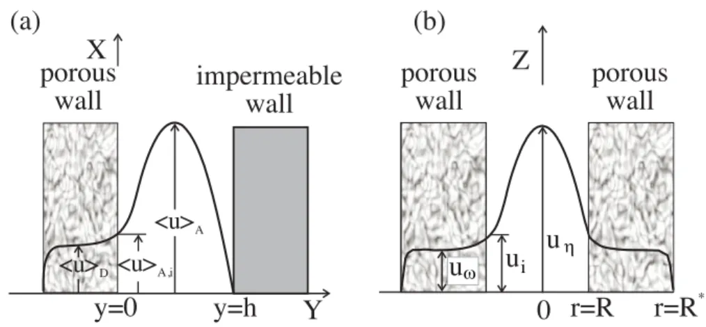
where μis the local fluid viscosity,K is the local permeability of the porous medium,uD is the Darcy velocity vector, defined as an averaged velocity over a representative volume of the porous medium, andpfV is the pore averaged pressure. Analytical description of flow for a composite region has been attempted in a number of simple geometries. For one-dimensional flow through a channel, of widthh, bounded by a saturated porous medium on one side, and by an impermeable wall on the other side [Fig.1(a)], the resulting velocity fields are usually estimated from two different theoretical approaches. In the first approach, often termed Brinkman’s equation [16], the interface between the saturated porous medium and the adjoining channel is treated as a part of a continuum. A macroscopic shear term is added to Darcy’s law to account for the velocity gradients present at the interface
−μ
KuV +μ˜∇
2u
V =∇p f
V, (2)
FIG. 1. Diagrams and relevant definitions describing (a) one-dimensional fluid flow and (b) in flow plane cross section of a fully developed axially symmetric fluid flow in a porous medium with a model sample geometry. See the text for further explanations.
In the second approach, developed in [4], velocity profiles in the channel are found by solving the Navier-Stokes equation with a no-slip boundary condition imposed on the velocity at the impermeable wall and with a slip, or hydrodynamic, boundary condition imposed on the velocity at the interface with porous medium. The hydrodynamic boundary condition relates the interfacial shear to the slip velocity at the interface according to
duA dy
y=0+
= √α
K(uA,i−uD), (3)
whereα, the empirical slip coefficient, is a dimensionless quantity that supposedly depends on the structure of the porous medium,y =0+indicates that the velocity gradient is evaluated at the interface and towards the adjoining channel in the direction transverse to flow, uA is the area-averaged component of velocity in thexdirection (i.e., along the flow),uA,iis the area-averaged interfacial or slip velocity evaluated aty =0,uDis the Darcy velocity, andKis the permeability of the porous medium. The resulting velocity distribution for this model is given elsewhere [4,17,18].
The validity of both approaches in the interpretation of experimental flow data has been extensively studied [19]. For a complete analysis of the application of either approach to the description of flow in spatially heterogeneous model porous media the reader should refer to [19–21]. The major problem in these two approaches was the overdetermination of the physical problem in an attempt at the continuous matching of shear across the interface [21]. This issue was overcome in the approach proposed in [6,7], where the use of sophisticated averaging technique matched the Brinkman-extended Darcy law to the Stokes equations by requiring a discontinuity in the stress but retaining continuity in velocity. The boundary condition was termed the stress jump boundary condition and the use of discontinuity in the stress at the interface circumvented the overdetermination of the physical problem as was pointed out by Neld [22].
A. Fully developed axially symmetric flow in a clear channel bound to a saturated porous medium
The problem was treated before [8] and basic flow equations are stated here rather than derived. Closely following [8], we see that in the open fluid region, orηregion, the equation of fluid motion expressed in dimensionless variables is given by
d2u
η dr2 +
1 r
duη
dr = −R, 0r1, (4)
while in the porous medium, orωregion, the dimensionless expression
d2u
ω dr2 +
1 r duω dr = 1 γ2 −R+
1 DaRuω
, 1r R
∗
R , (5)
holds, where
γ = μ
eff
μf
, r= r˜
R, DaR = K
R2, R = −
R2
μfU pff
dx˜ , (6)
where ˜ris the radial coordinate (in m),ris the dimensionless radial coordinate,Ris the radius of the open channel (in m),R∗is the outer radius of the cylindrical porous medium (in m), DaR is the Darcy number for a cylindrical channel,R is the dimensionless pressure gradient in the direction transverse to flow for a cylindrical channel, μf is the fluid viscosity (in kg m−1s−1),μeff is the
effective viscosity in the Brinkman term (in kg m−1s−1),U is the reference velocity (in m s−1),
pff is the intrinsic average pressure (in Pa), and ˜x is the streamwise coordinate (in m). The following boundary conditions are utilized:
duη
dr =0 atr=0, uω=0 atr= R∗
R,
uη =ui atr=1, uω=ui atr=1. (7) The solution of Eqs. (4) and (5) with the boundary conditions (7) is given by
uη =ui+ R
4 (1−r
2) at 0r 1, (8)
uω=A3I0
r
γ√DaR
+B3K0
r
γ√DaR
+RDaR at 1r R∗
R , (9)
where the coefficientsA3andB3are given by
A3= −
RDaR I0(ψ2)
−K0(ψ2)
I0(ψ2)
uiI0(ψ2)−RDaR[I0(ψ2)−I0(ψ1)]
K0(ψ1)I0(ψ2)−K0(ψ2)I0(ψ1)
(10)
and
B3=
uiI0(ψ2)−RDaR[I0(ψ2)−I0(ψ1)]
K0(ψ1)I0(ψ2)−K0(ψ2)I0(ψ1) , (11) respectively, with
ψ1=
1
γ√DaR, ψ2= R∗
R 1
To evaluate the dimensionless interfacial velocityui, the stress boundary condition given by
γ2duω dr −
duη dr =
β √
DaRuω atr=1 (13)
is used [6,7]. Then the expression forui becomes complicated and is given by [8]
ui =
−γ2ψ1RDaR
I1(ψ1)
I0(ψ2)+
R 2 +γ
2ψ
1RDaR
K1(ψ1)+K0(ψ2)
I1(ψ1)
I0(ψ2)
× I0(ψ2)−I0(ψ1)
K0(ψ1)I0(ψ2)−K0(ψ2)I0(ψ1)
×
β √
DaR +γ
2ψ
1
K0(ψ2)I1(ψ1)+K1(ψ1)I0(ψ2)
K0(ψ1)I0(ψ2)−K0(ψ2)I0(ψ1)
−1
. (14)
B. Pore-scale LBM of axially symmetric flow in a clear channel within a saturated porous medium
To avoid difficulties involved with a specific treatment of the interface and an effective viscosity parameter (as described above), one can apply pore-scale LBM to treat this problem. One usually starts from the microscopic approach that is based on the Navier-Stokes equations governing the dynamics of fluid flowing both in the pure fluid region and in the heterogeneous porous region on the pore scale. This is equivalent to the single domain formation on the microscopic scale across the whole domain. One of the advantages of this approach compared to the approaches described in Sec. II is the elimination of any specific treatment of the interface. However, the challenge is in the accurate representation of the complicated pore structure on the pore-scale level. This requires experimental and demanding computational resources. Experimentally, one needs to use x-ray microcomputed tomography (XμCT) to obtain and to further reconstruct the complicated 3D structure of a porous medium under study. Computationally, the LBM method has been established as an efficient algorithm for simulating fluid flows, especially for flow of fluids through complex porous media [23]. The reconstructed 3D digital structure, where each voxel represents a portion of the original porous material, is usually mapped into computational lattice nodes in LBM [24].
In this study, LBM employs the single-relaxation-time lattice Bhatnagar-Gross-Krook collision model [25,26] that can be written as
fi(x+eiδt,t+δt)−fi(x,t)
streaming
= −1
τ[fi(x,t)−f eq i (x,t)]
collision
, (15)
wherexdenotes the position of lattice node,τdenotes the relaxation time, andfidenotes the particle distribution function which streams along the discrete lattice velocity vectorei; the right-hand side of Eq. (15) represents the rate of change offi resulting from collisions between the incomingfi and the equilibrium particle distribution functionfieq. The relaxation timeτthat controls the rate of approach to equilibrium is chosen to be unity to reduce the viscosity dependence [27] in the whole fluid simulation. Hereδt is assumed to be unity. The functionfieq depends on only the fluid local densityρand velocityuand has the form (the three-dimensional d3q19 model)
fieq =tiρ
1+3(ei·u)+92(ei·u)2−32u·u
, (16)
where
The fluid densityρand velocityuon each lattice node are evaluated through the moments of the particle distribution functions with respect toei,
ρ= i=0
fi, (18)
ρu=
i=0
fiei. (19)
A Chapman-Enskog procedure can be applied to Eq. (15) to derive the macroscopic governing equations of fluid flows with second-order accuracy. They are given by the continuity and Navier-Stokes equations
∇·u=0, (20)
ρ
∂u
∂t +u·∇u
= −∇p+μ∇2u. (21)
Therefore, through pore-scale lattice Boltzmann modeling we can directly simulate the behavior of fluids flowing inside both the clear fluid region and the adjacent porous medium.
III. MATERIALS AND METHODS
A. NMR methods
NMR and MRI velocimetric methods and their applications to study fluid flow have been extensively reviewed [9,12,15,28]. In the present work, the motion encoding was achieved by a phase method [29]. Briefly, a pair of field-gradient pulses of different effective polarity is incorporated into an NMR pulse sequence in addition to rf excitation which produces transverse magnetization. These field-gradient pulses of durationδ and magnitudegare usually separated by a time delay. The application of the first gradient pulse changes the local magnetic field according toB=B0+rg,
whereBis the local magnetic field andris the position vector. If a collection of magnetically active spins was at positionr0flowing with velocityv, then transverse nuclear magnetization undergoes
a phase shift ofγgr0δ. During a time interval, the nuclei move to a positionr=r0+v. As a
result, at the end of the second gradient pulse the transverse magnetization has the phase shift of γg(r0−r)δ, or−vγgδ. The transverse magnetization produced by this collection of magnetically
active spins averaged through a volume elementd3(r0−r) can be expressed as
E(q,r,)=
V
P(r0−r;,r)exp[−iq(r0−r)]d3(r0−r), (22)
whereP(r0−r;,r) is the probability for an ensemble of nuclei to be displaced byr0−rfromr0
during, or a propagator, andq=γ δgis a wave vector conjugate to the space of spin displacement
r0−r. For the case of unrestricted isotropic diffusion superimposed on uniform flow Eq. (22) can
be solved and a solution is given by [30]
E(q,r,)∼=E0exp
−q2D
−δ
3
+iqv(r)
, (23)
whereE0is the initial intensity or the initial spin density,Dis the apparent dispersion coefficient,
andv(r) is the local velocity. Analyzing experimental intensities for a few values ofγgδby Eq. (23), one can estimate values ofE0,v, andD.
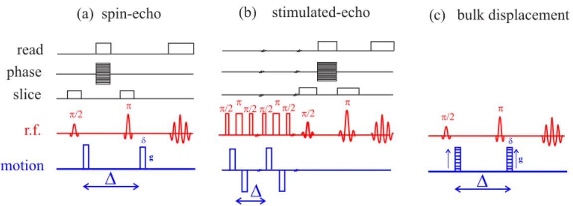
FIG. 2. Timing diagrams of flow measurements using (a) spin-echo and (b) stimulated-echo MRI protocols. (c) Timing diagram for measuring bulk displacement spectra by NMR. Motion encoding gradients are applied in the direction of flow. Bars indicate that the time axes are not continuous in (b).
function ofγgδand obeys Eq. (23). Therefore, velocity values can be determined for each individual pixel by fitting the field-gradient-dependent intensity of the pixel to Eq. (23). The intensity of each pixel is then replaced by a corresponding velocity value to yield two-dimensional velocity maps. The same approach is used to produce spin densityE0and dispersionDmaps. Two-dimensional velocity maps can be further analyzed to produce radial velocity profiles. The analysis is simply based on azimuthal averaging of velocities extracted from the maps, assuming axial symmetry of the flow. A complete description of this method is given elsewhere [31].
Timing diagrams of velocimetric MRI protocols used in the present work are displayed in Fig.2. The spin-echo protocol shown in Fig.2(a)was used to characterize fast fluid flow in the open channel and in the vicinity of the interface with the porous medium. To characterize fluid flow in the porous medium whereT2is greatly shortened by diffusion of fluid in the porous medium, the stimulated-echo
protocol, shown in Fig.2(b), was preferred. Since this protocol allows forzstorage of magnetization during the NMR flow experiment, the observation time in this protocol is limited only by spin-lattice relaxation,T1. Since the dephasing of spin coherence is not a limiting factor in this protocol, the
NMR data can be measured for larger values of, the time between field-gradient pulses. As a result, the measured velocity fields will reflect the motion of spin particles that traveled two or three pores before data were sampled [10]. This is beneficial for the characterization of temporally averaged percolating flow which occurs in a porous medium.
For both spin-echo and stimulated-echo experiments, planar sample cross sections were imaged transverse to the direction of flow. Flow encoding was performed for 10–12 and for 6–8 different values of applied field gradient q in spin-echo and stimulated-echo experiments, respectively. Image size was kept at 256×256 pixels for spin-echo and 128×128 pixels for stimulated-echo experiments, thus the total three-dimensional data acquisition required from 10 to 15 and from 18 to 24 h, respectively. The larger experimental time in the latter experiment is explained by longer (approximately 100 times)values, the time between field-gradient pulses, and larger signal averaging. The field of view (FOV) was 3.0×3.0 cm2in both experiments.
Bulk displacements were measured using the timing diagram displayed in Fig.2(c). The spectra were measured with 256 flow encoding gradients at different values of flow encoding times. The resulting two-dimensional data were processed by Fourier transformation in spectroscopic andq
directions with no zero fill in either direction of the Fourier transforms. The resulting spectrum in theqdirection (second dimension) displays all coherent displacements that occur during the chosen flow evolution time. Details of this approach can be found in [28].
signal-to-noise ratio was achieved after one scan; a 20 Hz linewidth of a1H single water peak was
readily achieved after successful shimming. The lengths ofπ/2 hard pulse1H pulse and sinc-shaped selective pulse were 20μs and 1.5 ms, respectively.
B. Experimental setup
A reticulated polyurethane foam was used as a model porous medium. The material is designed for water filtering and is characterized by a spongelike structure where a nearly rigid polymer network comprises large and open pores. The pore count is approximately four pores per cm (dpav=0.25 cm) and permeability data for a similar material can be found elsewhere [5]. A sample porous medium was manufactured from bulk material in the shape of a cylinder which was 55 mm in length and 24 mm in diameter and was used to characterize displacement in the bulk of this porous medium as it happens well far away from the interface with an open channel. Another porous medium was manufactured from this material with exactly the same shape, though a cylindrical channel of 7 mm in diameter was cut through the sample coaxial with its central axis. To prevent fluid momentum transport across the interface a rigid tube [(7±1) mm outer diameter and (5±1) mm inner diameter] made from impermeable polymer (G10) was inserted into the channel. Bulk flow measurements were performed in the porous medium without the channel, while MRI velocimetry measurements were performed in the porous medium with the channel and with the polymer tube inserted into the channel.
Boiled distilled water with a trace amount of antiseptic was used in this study as a model fluid. Water was boiled to minimize bubble formation in the porous medium during flow experiments and traces of antiseptic (sodium azide) were also added to prevent bacteriological contamination of the water. The porous media were incorporated into a custom-made plastic column with outlets on the top and the bottom of the column to provide circular flow through the porous medium. The column was mounted in the middle of the superconducting magnet and Tygon tubing was used to connect the column with a water reservoir and a pump. The desired flow rate was delivered by the pump placed between the entrance to the column and water reservoir. The flow in the column was directed from the bottom to the top in order to facilitate bubble removal from the porous medium during the experiment.
C. X-ray microcomputed tomography
The sample was imaged using a high-resolution x-ray 3D computed tomography microscope instrument, model VeraXRM-510 (manufactured by Xradia Inc, Pleasanton, CA, USA). The voxel resolution was 5.5μm. The 3D structure of the porous medium was further constructed by stacking together individual 2D images.
IV. RESULTS AND DISCUSSION
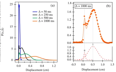
The character of transport in a bulk porous medium is usually reflected in a spectrum of molecular displacements Pav(r,) measured over a time interval using the generalized NMR protocol displayed in Fig. 2(c). The shape of the spectrum of molecular displacements strongly depends upon the quantityv/dp, whereis the time allowed for displacements to occur,vis the interstitial fluid velocity, anddpis the averaged pore size [27; 28; 29]. For smallv/dp, the propagator is very asymmetric and reflects the instantaneous velocity distribution in channels and pores of the medium. For large v/dp, the propagator usually becomes nearly Gaussian. For intermediatev/dp, the displacement spectrum can be very complex with multimodal propagators reflecting different modes of transport in the porous medium [9,10].
The character of transport in the bulk porous medium sample used in this study can be understood from examining the temporal dependence of the longitudinal probability displacement distributions of fluid molecules in a single-phase incompressible flow of water in a reticulated foam cylinder at Re≈13 determined using the average pore velocity over a length scale ofdav
probability
Displacement (cm) Displacement (cm)
FIG. 3. Displacement spectra (propagators) for water flow in a bulk reticulated foam at Re≈13 for different
times: (a) measured normalized propagators using NMR protocol displayed in Fig.2(c)(solid lines) and (b) measured (symbols) and simulated (dashed lines) with a bimodal Gaussian function and deconvoluted normalized propagator at=1000 ms.
zis the net fluid particle displacement over time in the direction of flow. It was found that at =1000 ms the displacement probability distribution can be simulated with a bimodal Gaussian propagator, as shown in Fig.3(b). The first peak is located at around zero value and corresponds to fluid molecules located in low-velocity zones such that displacements occurring there during the measurement time are small compared to the pore size. Using a velocity of 0.0026 cm/s and a time of 1 s, we estimate that the length scales of these small local areas are on the order of 4.3×10⁻²cm. The average pore size of the reticulated foam, being 2.5×10⁻¹cm, is approximately
one and half orders of magnitude higher. Since the presence of such small pores can hardly be expected in this material, the appearance of the first peak can be plausibly explained by the displacements of water molecules inside the polymeric material that comprises the foam. The fact that water penetrates into the polymeric core of the foam is also evident from the swelling of the foam upon prolonged exposure to water. Similarly shaped propagators were also observed for flow in a bed of permeable spheres [32]. The faster displacing peak can be described by Gaussian distribution and this can be explained by reaching the→ ∞limit where diffusing molecules probe the connectivity of the pore space only. In regions where the displacement probability distribution lies between short-time and long-time behavior, the transport appears to be intermediate in character between dispersion and diffusion and between convection and dispersion, leading to a complicated form of the propagator. Similar effects have been reported before [10]. The bimodal Gaussian behavior is apparent for all <1000 ms and, in principle, reflects similar transport character in the bulk reticulated foam within the probed flow evolution times.
R
0.0 0.5 1.0 1.5 2.0 2.5 3.0 3.5 r/R
0.85 0.90 0.95 1.00 1.05
φ
, porosity
(b)
R=0.5 cm
( c)
0 2.5
2.5
x (cm)
y (cm)
(a)
FIG. 4. (a) Example of an individual 2D XμCT image of the foam with relevant length scales. (b) A 3D visualization of the cylindrical porous foam with a coaxial clear-cut circular channel reconstructed using a series of the segmented 2D XμCT images displayed in (a). The solid matrix is shown in yellow, while transparent designates pore spaces. The radius of the clear channel in this porous medium produced specifically for XμCT was approximately 0.5 cm. (c) Azimuthally averaged porosity profile produced from the reconstructed porous medium displayed in (a).
be determined using segmented binary XCT images. Furthermore, the porosity in the radial direction can be determined through azimuthal averaging. Figure4(b)shows an azimuthally averaged porosity profile that was obtained using an ensemble average for ten different cross-sectional images. The porosity inside the clear fluid region attains a value of unity, while the porosity inside the adjacent porous region fluctuates, which indicates the expected variability and complexity of the pore space, especially in the near interface region.
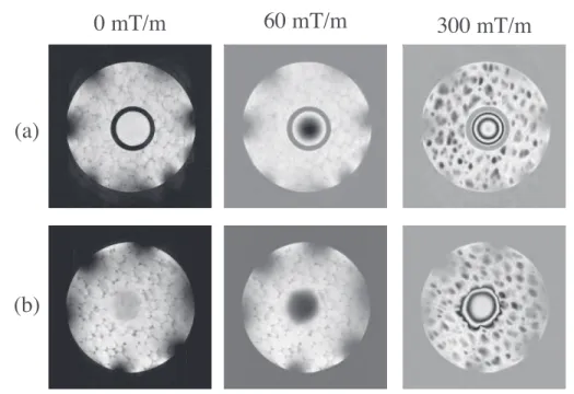
FIG. 5. Phased flow images as a function of the applied field gradientq(a) in the absence of the fluid momentum transport across the interface (the rigid tube is inserted into the channel) and (b) with the momentum transport across the interface (the rigid tube is taken out). Flow encoding was performed by spin-echo protocol in the direction of flow for a few cross sections across the height of the porous medium. The raw matrix size was 256×256 and the FOV was 3×3 cm2with a slice thickness of 0.1 cm. The flow encoding timewas
kept to 8 ms as no outflow effects influenced the shape of velocity profiles when a volumetric flow rateQof 1.4 cm3/s was used.
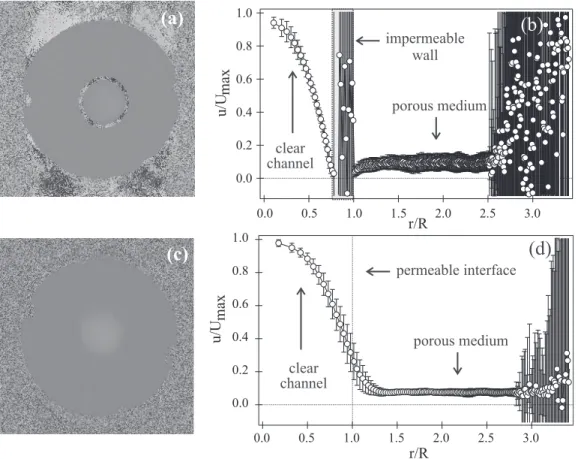
image. This behavior is most apparent at the highest field gradient for the flow in the clear channel in the absence of the fluid momentum transport across the interface [Fig.5(a)], where highly symmetric phase rings are the consequence of well-developed Poiseuille flow. When fluid momentum transport across the interface occurs, the symmetry in the phase ring structure gets distorted [Fig.5(b)] as the presence of momentum transfer across the permeable interface creates additional velocity gradients. Two-dimensional velocity maps are displayed both in the absence [Fig.6(a)] and in the presence [Fig.6(c)] of the fluid momentum transport across the interface. A Gaussian distribution of dynamic displacements over a chosen time intervalwas confirmed by bulk displacement measurements (Fig.3) and was used for velocity calculations as described in Sec.III. The radial velocity profiles were produced from these maps by azimuthal averaging with a fixed bin size in the radial direction (0.226 mm), as explained in [31]. The error bars, calculated as standard deviations in each bin, are also shown for each averaged velocity value.
porous medium
clear channel
impermeable wall
(a)
(c)
porous medium
clear channel
permeable interface
(d)
1.0
0.8
0.6
0.4
0.2
0.0
u/U
max
3.0 2.5 2.0 1.5 1.0 0.5 0.0
r/R
(b)
1.0
0.8
0.6
0.4
0.2
0.0
u/U
max
3.0 2.5 2.0 1.5 1.0 0.5 0.0
r/R
FIG. 6. (a) and (c) Velocity maps and (b) and (d) corresponding azimuthally averaged radial velocity profiles (a) and (b) in the absence and (c) and (d) in the presence of the fluid momentum transport across the interface. The greater error in velocities in (b) is due to the larger bin size used in azimuthal averaging. The increase of errors in velocities near the wall in both experiments is induced by the distortions in image intensity due to the rf inhomogeneity in the coil as mentioned elsewhere in the paper. Larger errors in velocities in (a) in 0.85< r/R <1.14 are due to the absence of the collected NMR signal from the location of the rigid tube placed inside the channel.
as can be seen from the radial velocity profile displayed in Fig.6(d). In the absence of the rigid wall the transport of fluid momentum across the interface occurs and results in a slip in velocity at the boundary with the porous medium. The velocity reaches a constant value atr greater thanR, the radius of the channel. This flow behavior is consistent with theoretical considerations outlined in Sec.II.
0.5
1.0
0.0 0.5 1.0 1.5 2.0 2.5 3.0 3.5
r/R
0.0
0.2
0.4
0.6
0.8
1.0
u
/
U
max0.5
1.0
0.0 0.5 1.0 1.5 2.0 2.5 3.0 3.5
r/R
0.0
0.2
0.4
0.6
0.8
1.0
u
/
U
max(a) (b)
(c) (d)
FIG. 7. (a) and (c) LBM simulated normalized velocity maps and (b) and (d) corresponding normalized azimuthally averaged radial velocity profiles (a) and (b) in the absence and (c) and (d) in the presence of the fluid momentum transport across the interface. The blue line in (b) represents the analytical solution of the velocity profile for Poiseuille flow. The irregular white shapes in (a) and (c) are the foam.
is also displayed in Fig. 7(b). Velocities in the profile vary across the porous region with these variations corresponding to fluctuations in the sample porosity in the radial direction, as shown in Fig.4(b). Furthermore, these variations in velocities are expected, as in this work, as velocities inside an individual pore are solved directly and should be different from the volume-averaged uniform velocities profile derived from the phenomenological Darcy law (1). Moreover, the velocity attains its highest value in the profile at aroundr/R∼2.5 and this corresponds to the highest porosity achieved after the azimuthal averaging, as evident from the radial porosity profile displayed in Fig.4(b).
1.0
0.8
0.6
0.4
0.2
0.0
u/Umax
3.0 2.5 2.0 1.5 1.0 0.5 0.0
r/R
porous medium clear channel
permeable interface
1 mm 5 mm 20 mm
FIG. 8. Effect of spatial averaging on flow in the channel with a permeable wall at the volumetric flow rate
Q=2.25 cm3/s. Radial velocity profiles were produced by azimuthal averaging with a bin size of 400 from
velocity maps produced by spin-echo flow experiments, acquired in 256×256 matrices for 12 different values of field gradients with=8 ms and a FOV of 3×3 cm2.
the boundary condition on the tangential velocity component of the free fluid at the interface is not explicitly specified, the pore-scale modeling clearly predicts slip at the permeable interface with the porous medium. Further, it can be observed from Fig.7(d)that the slip velocity value of the free fluid at the interface is considerably greater than the averaged velocity value within the Darcy section. This indicates that the flow rate through the free fluid region adjacent to a permeable porous material under the same condition is significantly greater that that of the fluid region adjacent to a nonpermeable wall.
A. Spatial averaging and mass balance assessment
To assess the influence of structural fluctuations in the porous bed on velocity fields measured in the MRI flow experiment, planar velocity maps were collected as a function of slice thickness at a flow rate ofQ=2.25 cm3/s. Azimuthally averaged radial velocity profiles determined from this set
of experiments are displayed in Fig.8. Figure8shows that radial velocity profiles are independent of the chosen slice thickness used in this series of flow experiments. The independence of velocity distributions on the slice thickness is probably explained by the relative structural homogeneity of the porous medium. Moreover, the result also suggests that any fluctuations in velocities that might be induced by structural inhomogeneities are not measurable during the chosen flow encoding time =8 ms, in fact the shortest flow encoding time used in this study.
In addition, the velocity profile obtained from the 1 mm slice was used to check the mass balance in an MRI flow experiment. The calculated flow rate obtained by radial integration of the 1 mm profile wasQ=2.5 cm3/s compared toQ=2.25 cm3/s determined by timed collection. The difference between the two values can be explained by difficulties in determining correct values of velocities near the column wall induced by the poor image quality at the edge due to rf inhomogeneity of the coil, but in all the difference between the measured and the calculated mass transport was within 10%.
B. Temporal averaging in MRI flow experiments
1.2
1.0
0.8
0.6
0.4
0.2
0.0
u/U
max
3.0 2.5 2.0 1.5 1.0 0.5 0.0
r/R impermeable interface
(a)
= 8 ms = 500 ms
1.2
1.0
0.8
0.6
0.4
0.2
0.0
u/U
max
3.0 2.5 2.0 1.5 1.0 0.5 0.0
r/R interface
(b)
= 8 ms = 500 ms
FIG. 9. Effect of temporal averaging on flow in the channel (a) decoupled from and (b) coupled to the flow in the porous medium at a volumetric flow rateQ=1.4 cm3/s. The=8 ms profiles were produced from
the spin-echo experiments acquired in 256×256 matrices with 12 flow encoding gradients. The=500 ms profiles were produced from the stimulated-echo experiments acquired in 128×128 matrices with 8 flow gradients. The FOV in both experiments was 3×3 cm2with a slice thickness of 1 cm.
The measurements were first performed with the impermeable tube inserted into the channel to decouple flow in the channel from flow in the porous medium. No difference within experimental error [Fig.9(a)] between the velocity profiles measured at=8 ms and=500 ms was observed. The absence of temporal effects in velocity profiles can be explained as follows. When flow in the clear channel is no longer coupled to the porous medium and is in principle fully developed atQ=1.4 cm3/s no difference in velocity fields in the clear channel associated with the entry
effects should be observed by the time the fluid reaches the detection region. This is supported by a simple estimate of the entry lengthLhof 10.692 cm for Rech=324 determined using the diameter of the clear channel at this volumetric flow rate. This means that it takes about 2 s for the flow to get established and this clearly happens as the detection region is located inside the magnet at a distance of 52 cm from the bottom magnetic plate. In the porous medium, a spin particle displaces approximately 0.2 cm atQ=1.4 cm3/s during=500 ms. This distance is less than the average pore sizedpav=0.35 cm. To observe temporal flow fluctuations in the porous medium a particle should be allowed to percolate distances of the order of at least two or threedp; therefore, profiles in the porous medium should not be different within the chosen flow encoding times. This assumption is clearly confirmed by the velocity distributions in the porous medium displayed in Fig.9(a).
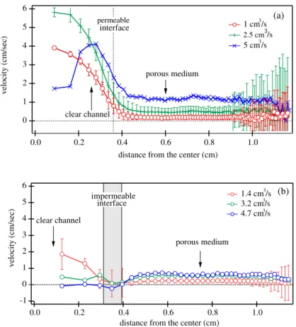
FIG. 10. Azimuthally averaged radial velocity profiles (a) in the presence of transverse permeability discontinuity and (b) in the absence of the discontinuity in permeability as a function of the adjusted flow rate. The velocity fields were measured using the stimulated-echo protocol, with a raw acquisition matrix size of 128×128, a FOV of 3×3 cm2, and a slice thickness of 0.5 cm at=500 ms. The measured slip velocities
in (a) were 1.0±0.3, 1.6±0.5, and 2.5±0.8 cm/s for flow rates of 1, 2.5, and 5 cm3/s, respectively.
fields in the porous medium also differ within 10% of each other and are probably associated with similar instabilities in the flow rate. Moreover, temporal averaging for longer time results in a more homogeneous velocity profile and can be explained by averaging individual velocity fluctuations over a longer observational time. Despite these fluctuations, temporally averaged, rather than snapshot, velocity measures are more appropriate for these complex systems, as they allow for a better estimate of velocities in the boundary region where additional fluctuations in velocity values might be induced by, on the average, less thandav
p in the porous medium, well away from the boundary region pore size. This decrease indpin the boundary region is associated with the modification of the surface of the porous medium during the manufacturing of the clear channel.
C. Azimuthally averaged radial velocity profiles under varying mass transport
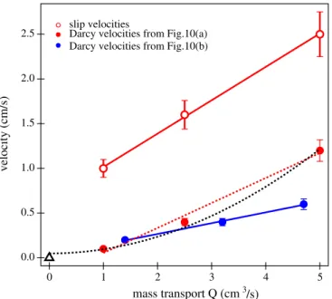
FIG. 11. Slip and averaged Darcy velocities as a function of the increased mass transport in the presence of transverse permeability discontinuity (red) and in the absence of the discontinuity in permeability (blue). Note the quadratic Darcy velocity dependence on the increased mass transport (dashed black line) in the presence of transverse permeability discontinuity. The quadratic analysis was performed assuming that no slip velocities are observed at zero flow rate. Hence the zero point (black open triangle) has no error bars.
likely was caused by the removal of faster flowing excited spins from the rf coil detection region during the time course of the NMR experiment.
This also explains the distorted shape of the velocity profiles in the open channel in both cases with no reliable velocity measures with the increased mass transport. In addition, a greater error in Fig.10(b)in the open channel is also due to the increased bin size in the radial averaging procedure as the bin size was decreased to 100 for the clarity of presentation. In the absence of the momentum transport across the interface [Fig.10(b)] the boundary velocities at the open channel side of the interface and at the porous medium side of the interface were zero and were independent of the flow rate, as expected when the no-slip boundary condition is imposed. No slip at either side of the interface was observed.
Transverse permeability discontinuity promotes fluid momentum transport across the interface that manifests in the apparent slip in velocities at the interface. Measurable nonzero fluid velocities [Fig.10(a)] at the interface were present at all flow rates studied. Slip velocities were also increased as a function of flow rate, as shown in Fig.11.
0.45 0.40 0.35
0.30 0.25 0.20 0.15
0.10
u/Umax
1.20 1.15 1.10 1.05 1.00 0.95 0.90
r/R
1.0
0.8
0.6
0.4
0.2
0.0
u/U
max
3.5 3.0 2.5 2.0 1.5 1.0 0.5 0.0
r/R interface
experimental data
fit using exact solution to the problem fit using LBM
FIG. 12. Comparison of radial velocity profile in the presence of fluid momentum transport across the permeable interface atQ=1.4 cm3/s (open symbols) with Eq. (8) at r < R, Eq. (9) at r > R(red), and
LBM (blue). Velocity fields were temporally averaged within=8 ms. The inset shows zoomed in boundary behavior of the exact solution to the problem and LBM modeling. Note a better match to the experiment for LBM.
D. Comparison of experimental velocity fields in the presence of the transverse permeability discontinuity to theoretical and LBM velocity fields
The velocity field atQ=1.4 cm3/s was compared to the velocity fields constructed using Eqs. (8)
and (9) and LBM. These computational velocity fields were compared with experimental data as displayed in Fig.12. Both approaches provided a flow description that coincided very well with the experiment in both the open channel and the porous medium. The major difference between the two models was in the description of flow behavior in the boundary region.
As can be seen from the inset in Fig.12, the theoretical flow behavior derived using both Eqs. (8) and (9) shows an almost stepwise change in the velocities when the boundary changes to the open channel. This reflects the sensitivity of this combined approach to the choice of the boundary condition or to the averaging procedure as discussed in the Introduction. The velocity profile derived using LBM demonstrates a smooth transition in velocities from the boundary to the open channel, thus confirming the assumption that the boundary velocities can be evaluated using this method without any assumption of the boundary velocities.
V. CONCLUSION
ACKNOWLEDGMENTS
This work was supported by the Engineering and Physical Sciences Research Council (Grant No. EP/J008753/1); and the Medical Research Council (Grant No. G0900785). G.E.P. and T.M. also express their gratitude to the in-house research program in National High Magnetic Field Laboratory, Tallahassee, USA for the financial support of this project.
[1] J. Bear,Dynamics of Fluids in Porous Media(Elsevier, New York, 1972).
[2] A. E. Scheidegger,The Physics of Flow through Porous Media(Macmillan, New York, 1972). [3] R. E. Collins,Flow of Fluids through Porous Materials(Reinhold, New York, 1961).
[4] G. S. Beavers and D. D. Joseph, Boundary conditions at a naturally permeable wall,J. Fluid Mech.30, 197(1967).
[5] R. C. Givler and S. A. Altobelli, A determination of the effective viscosity for the Brinkman-Forchheimer flow model,J. Fluid. Mech.258,355(1994).
[6] J. A. Ochoa-Tapia and S. Whitaker, Momentum transfer at the boundary between a porous medium and a homogeneous fluid-I. Theoretical development,Int. J. Heat Transfer38,2635(1995).
[7] J. A. Ochoa-Tapia and S. Whitaker, Momentum transfer at the boundary between a porous medium and a homogeneous fluid-II. Comparison with experiment,Int. J. Heat Transfer38,2647(1995).
[8] A. V. Kuznetzov, Analytical investigation of the fluid flow in the interface region between a porous medium and a clear fluid in channels partially filled with a porous medium,Appl. Sci. Res.56,53(1996). [9] J. D. Seymour and P. T. Callaghan, Generelized approach to NMR analysis of flow and dispersion in porous
media,AIChE J.43,2096(1997).
[10] M. H. G. Amin, S. J. Gibbs, R. J. Chorley, K. S. Richards, T. A. Carpenter, and L. D. Hall, Study of flow and hydrodynamic dispersion in a porous medium using pulsed-field-gradient magnetic resonance, Proc. R. Soc. A453,489(1997).
[11] R. M. Cotts, M. J. R. Hoch, T. Sun, and J. T. Marker, Pulsed field gradient stimulated echo methods for improved NMR diffusion measurements in heterogeneous systems,J. Magn. Reson.83,252(1989). [12] V. Rajanayagam, S. Yao, and J. M. Pope, Quantitative magnetic resonance flow and diffusion imaging in
porous media,Magn. Reson. Imaging13,729(1995).
[13] P. Mansfield and B. Issa, Fluid transport in porous rocks I: EPI studies and a stochastic model of flow, J. Magn. Res. A122,137(1996).
[14] K. J. Packer and J. J. Tessier, The characterization of fluid transport in a porous solid by pulsed gradient stimulated echo NMR,Mol. Phys.87,267(1996).
[15] P. T. Callaghan, Rheo-NMR: Nuclear magnetic resonance and the rheology of complex fluids,Rep. Prog. Phys.62,599(1999).
[16] H. C. Brinkman, A calculation of the viscous force excreted by a flowing fluid on a dense swarm particles, Appl. Sci. Res. A1,27(1947).
[17] G. S. Beavers, E. M. Sparrow, and R. A. Magnuson, Experiments on coupled parallel flows in a channel and a bounding porous medium,J. Basic Eng.92,843(1970).
[18] G. S. Beavers, E. M. Sparrow, and B. A. Masha, Boundary condition at a porous surface which bounds a fluid flow,AIChE J.20,596(1974).
[19] M. Kaviany,Principles of Heat Transfer in Porous Media, Mechanical Engineering Series (Springer, New York, 1991).
[20] M. Sahraoui and M. Kaviany, Slip and no-slip velocity boundary conditions at interface of porous, plain media,Int. J. Heat Mass Transfer35,927(1992).
[21] D. A. Neld, The boundary correction for the Rayleigh-Darcy problem: Limitations of the Brinkman equation,J. Fluid Mech.128,37(1983).
[23] S. Chen and G. D. Doolen, Lattice Boltzmann method for fluid flows,Annu. Rev. Fluid Mech.30,329 (1998).
[24] C. Jin, P. A. Langston, G. E. Pavlovskaya, M. R. Hall, and S. P. Rigby, Statistics of highly heterogeneous flow fields confined to three-dimensional random porous media,Phys. Rev. E93,013122(2016). [25] P. L. Bhatnagar, E. P. Gross, and M. Krook, A model for collision processes in gases. I. Small amplitude
processes in charged and neutral one-component systems,Phys. Rev.94,511(1954).
[26] Y. H. Qian, D. d’Humières, and P. Lallemand, Lattice BGK models for Navier-Stokes equation,Europhys. Lett.17,479(1992).
[27] C. Pan, L.-S. Luo, and C. T. Miller, An evaluation of lattice Boltzmann schemes for porous medium flow simulation,Comput. Fluids35,898(2006).
[28] P. T. Callaghan,Principles of Nuclear Magnetic Resonance Microscopy(Oxford University Press, Oxford, 1991).
[29] E. L. Hahn, Spin echoes,Phys. Rev.80,580(1950).
[30] E. O. Stejskal and J. E. Tanner, Spin diffusion measurements: Spin echoes in the presence of a time-dependent field gradient,J. Chem. Phys.42,288(1965).
[31] S. J. Gibbs, K. L. James, and L. D. Hall, Rheometry and detection of apparent slip wall for Poiseuille flow of polymer solutions and particulate dispersions by nuclear magnetic resonance velocimetry,J. Rheol.40, 425(1996).
[32] D. Kandhai, D. Hlushkou, A. G. Hoekstra, P. M. A. Sloot, H. Van As, and U. Tallarek, Influence of Stagnant Zones on Transient and Asymptotic Dispersion in Macroscopically Homogeneous Porous Media,Phys. Rev. Lett.88,234501(2002).
[33] T. R. Brosten, S. L. Codd, R. S. Maier, and J. D. Seymour, Dynamic Length-Scale Characterization and Nonequilibrium Statistical Mechanics of Transport in Open-Cell Foams,Phys. Rev. Lett.103,218001 (2009).
[34] F. D. Doty, G. Entzminger, Jr., C. D. Hauck, and J. P. Staab, Practical aspects of birdcage coils,J. Magn. Reson.138,144(1999).