Nonhomogeneous Risk Rank Analysis Method for Security Network System

(1)

ISSN Online: 1913-3723 ISSN Print: 1913-3715

DOI: 10.4236/ijcns.2019.121001 Jan. 25, 2019 1 Int. J. Communications, Network and System Sciences

Nonhomogeneous Risk Rank Analysis Method

for Security Network System

Pubudu Kalpani Hitigala Kaluarachchilage

1*

, Chris P. Tsokos

2

, Sasith M. Rajasooriya

3

1_{Department of Mathematical and Physical Sciences, Miami University, Middletown, OH, USA} 2_{Department of Mathematics and Statistics, University of South Florida, Tampa, FL, USA} 3_{Department of Mathematics, University of Dayton, Dayton, OH, USA}

Abstract

Security measures for a computer network system can be enhanced with bet-ter understanding the vulnerabilities and their behavior over the time. It is observed that the effects of vulnerabilities vary with the time over their life cycle. In the present study, we have presented a new methodology to assess the magnitude of the risk of a vulnerability as a “Risk Rank”. To derive this new methodology well known Markovian approach with a transition proba-bility matrix is used including relevant risk factors for discovered and rec-orded vulnerabilities. However, in addition to observing the risk factor for each vulnerability individually we have introduced the concept of ranking vulnerabilities at a particular time taking a similar approach to Google Page Rank Algorithm. New methodology is exemplified using a simple model of computer network with three recorded vulnerabilities with their CVSS scores.

Keywords

Markov Chain, Vulnerability, Non Homogeneous Risk Analysis, Network Security, Google Page Rank

1. Introduction

A network system could have numerous vulnerabilities. We understand the process of generating vulnerabilities is highly stochastic and outcomes are hard to predict. Similarly the behaviors of attacks and attackers also have higher level of unpredictability. When considering a particular system based on the discov-ered vulnerabilities the analysis must consider the dynamic nature of the effect of vulnerabilities over time. As we observed in our previous researches [1] [2] [3] [4] [5], effect of the vulnerabilities vary with the time over their life cycle. Therefore, for a particular system, the most threatening vulnerability [6] [7] [8]

How to cite this paper: Kaluarachchilage, P.K.H., Tsokos, C.P. and Rajasooriya, S.M. (2019) Nonhomogeneous Risk Rank Anal-ysis Method for Security Network System. Int. J. Communications, Network and System Sciences, 12, 1-10.

https://doi.org/10.4236/ijcns.2019.121001

Received: December 11, 2018 Accepted: January 22, 2019 Published: January 25, 2019

(2)

DOI: 10.4236/ijcns.2019.121001 2 Int. J. Communications, Network and System Sciences

at time t1 might not be the same at time t2. Hence, it would be very useful to have analytical models to observe the behavior of the rank of vulnerabilities based on the magnitude of the threat with respect to time for a given network system.

Such ranking distribution over time would empower the defenders by giving the priority directions to attend on fixing vulnerabilities. In this paper we at-tempt to address this need.

In Section 2, the methodology of this new ranking approach is discussed with relevant introductions to Google Page Rank Algorithm and the Risk Rank Algo-rithm presented in this study. Section 3 illustrates the application of the pro-posed methodology with a model example step by step. Section 4 discusses the resulting risk ranks for vulnerabilities and their behavior over time. In Section 5, contributions of the study and conclusions are summarized.

2. Methodology

2.1. Google Page Rank Algorithm

This section provides a background for our quantitative analysis of risk rank al-gorithm method. Ranking web pages is an important function of an internet search engine [9] [10]. Google Page Rank Algorithm [11] is one of the most ac-curate and efficient page ranking methods in use. Methodology behind this algo-rithm will be briefly discussed below.

Output of this algorithm gives a probability distribution which is used to represent the likelihood that a person randomly clicking on links will arrive at any particular page. Using this method we can rank the likelihood of clicking on any web link. This can be calculated for any number of web links. In this algo-rithm, the sum of the page rank values of all the considered web links is equal to be one and it is assumed that the probability of selecting a web page initially is equal for any available option.

Google page rank algorithm simulates the clicking behavior of a web link in two ways. First is to visit a web link via an incoming link to the current web page and second way is to pick a web page randomly. Google page rank theory holds that any surfer who is randomly clicking on web links will eventually stop click-ing. At any of these stages, a damping factor d is the probability that the web surfer will continue surfing. Many researches have tested various damping fac-tors but in generally it is assumed that the damping factor will be set around 0.85.

Let p vt

( )

be the probability of visiting web page v at time t and v be a set of

all web pages under consideration. Here out v

( )

represents the set of web pages

in v with an outgoing link from v, and in v

( )

represents the set of incoming link to v. The page rank computation can be viewed as a Markov process whose states are pages and the links between pages represent state transitions. This computation is given in the Equation (1) below.

(

)

( )

_{( )}

( )

_{( )}

1 1

t t

t u V u in v

P u P u

P d d

V out u

(3)

Let, V be the number of pages considered. Surfer will stop clicking on any link with probability 1 − d. Since there are V number of pages and probability of visiting v from any page is equally likely, the probability for each case is equal to 1

V .

Here _{( )} t

( )

_{( )}

u in v

P u d

out u ∀ ∈

∗

∑

represents the case when the surfer continues

clicking links with probability d and goes to page v at time t + 1 from page u that has an incoming link to v.

Initially at t = 0, each page has the same ranking value probability which is equal to 1

V . Then iterations are executed over time until the stability is achieved. Once the probability distribution for each page becomes stable, consi-dering high to low probabilities ranks are assigned.

2.2. Risk Rank Algorithm

By developing the concept applied in Google Page Rank Algorithm here we in-troduce a ranking method for risk of vulnerabilities [10] [11] [12] [13] [14] in a network system.

To estimate the probabilities in Risk Rank Algorithm Markov model tech-niques can be applied similarly as in Google Page Rank Algorithm [11]. Howev-er thHowev-ere is a diffHowev-erence between web surfing behavior and CybHowev-er security attack-ing behavior. A web surfattack-ing user can randomly select a web page but in cyberat-tacks an attacker doesn’t have the same freedom. In web surfing user can arrive at any web page in one single step by using its URL. But attacker has many re-strictions. In computer network system an attacker doesn’t have the access to all vulnerabilities in the network system. To achieve attacker’s target state he must exploits several vulnerabilities in a particular order and enters in to the target system.

In the attacking process an attacker has two options. He can either continue or quit from his current path. If it is too difficult for him to achieve his goal state he can quit on the current path and try an alternative path by starting over from one of the set of initial states. Base on these assumptions here we propose our model to calculate the probability distribution of a given security attack model.

To obtain the risk rank [15] [16] [17] [18] we used the risk factor

R v t

( )

[2] [3] of each vulnerability at each state and calculated normalized risk factor matrix A(V, R) for the attack network system by using ϕ

( )

u v, transition

probabilities from state u to v. Thus, we can calculate transition probabilities using the equation

( )

₍

_{( )}

₎

( )

,

w out u

R v t u v

R w t

ϕ

∀ ∈

=

∑

.

Let Pk(v) be the probability of exploiting state 𝑣𝑣 at time k and V be a set of all states under consideration. Here out v

( )

represents the set of states in V with

(4)

The Risk rank computation can be viewed as a Markov process [1] [19] whose state are vulnerabilities and the links between vulnerabilities represent state transitions. This computation is given in the Equation (2) below.

( )

( ) (

)

( )

1

, , if is an intial state

, , if is not an intial state k

u in v k

k u in v

d

d P u u v v

I

P v

d P u u v v

ϕ

∀ ∈ +

∀ ∈

− 

∗ ∗ +

 = 

 ∗ ∗



∑

(2)

Let |I| be the number of initial states and attacker will stop his current path with probability 1 − d. Since there are |V| numbers of states and probability of exploiting v from any other state is equally likely, the probability for each case is

1

V .

Here in Equation (2)

d

∗

∑

_{∀ ∈}_{u in v}_{( )}

P u

_k

( )

∗

ϕ

( )

u v

,

represents the case when

the attacker continues his current path with probability d and attack to state v at time t + 1 from state u that has an incoming link to vulnerability v.

(5)

[image:5.595.240.507.170.542.2]

This procedure is illustrated by the following schematic diagram given in

Figure 1.

3. Illustration of Applying of the Risk Rank Algorithm

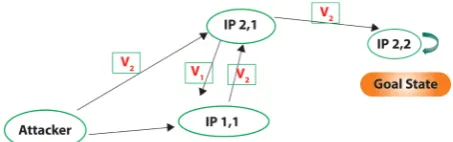
To illustrate the proposed analytical approach model that we have developed as discussed above, we considered a Network Topology [1] [4], given by Figure 2.

Figure 1. Key steps of the risk rank algorithm.

(6)

The computer network consists of two service hosts IP 1, IP 2 and an attackers workstation. Attacker is connecting to each of the servers via a central router. In the server IP 1 the vulnerability is labeled as CVE 2016-3230 and shall denote as

V1. In the server IP 2 there are two recognized vulnerabilities, which are labeled as CVE 2016-2832 and CVE 2016-0911. Let’s denote them as V2 and V3, respec-tively.

We proceed to use the CVSS score [12] [13] of the above vulnerabilities in our analysis.

The exploitability score (e(v) in Figure 2) and Risk Factor R(vj(t)) of each vulnerabilities as given in Table 1.

For example we can calculate the Risk Factor of V1 as follows.

( )

(

)

( ) ( )

R vj t

=

Y t

×

e vj

( )

(

1 )

0.1917010.383521 1

( )

0.00358ln ln

(

( )

)

8 R v t

=



_

t

−

t



_

×

and

( )

(

1 9

)

1.702 R v

=

Although our proposed algorithm can be applied to any form of network sys-tem, for simplicity we will use our host centric attack graph model [1] [4] [23]

introduced below to illustrate the process. The host centric attack graph is shown by Figure 3. Here, we consider that the attacker can reach the goal state only by exploiting V3 vulnerability. The graph shows all the possible paths that are available for the attacker to reach the goal state.

Note that IP1,1 state represents vulnerability V1 and states IP2,1 and IP2,2 represent vulnerabilities V2 and V3 respectively. Attacker can reach each state by exploiting the relevant Vulnerability.

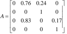
In this methodology for the Host Centric Attack graph [24] [25] we can have the Adjacency Matrix as follows. Applying the information given in Table 1, the matrix A(V, R) can be obtained as follows, where we can find the transition probabilities from one state to another state.

[image:6.595.260.487.540.611.2]

Figure 3. Host centric attack graph.

Table 1. Vulnerability scores.

Vulnerability Published date CVSS score e(vj) (tj) R(vj(t))

V1 (CVE 2016-3230) 6/15/2016 9 (High) 8 9 1.702

V2 (CVE 2016-2832) 6/13/2016 4.3 (Medium) 2.8 11 0.3667

(7)

0 0.76 0.24 0

0 0 1 0

0 0.83 0 0.17

0 0 0 1

A

 

 

=

 

 

Applying this normalized risk matrix into Algorithm 1, we can obtain steady state probabilities for each state in the network which represent risk of being ex-ploited [14] [15]. Results we obtained for each state are shown in Table 2.

Table 2 results are in the order of being exploited by attacker at time t. Order of vulnerabilities based on the rank we obtained is s1, s2, s3, s0. This result sug-gests that s1 has the highest likelihood of being attacked. This means at time t, s1 is the most vulnerable state. However according to Table 1 risk factor values for vulnerability v1 is 1.702 which is higher than the risk factor values of vulnerabili-ties v2 and v3. Therefore it is reasonable to assume that reaching state s1 from ini-tial state s0 (attacker’s state) by exploiting v1 vulnerability is easier than reaching states s2 and s3. Therefore, the risk rank of the state s1 is higher than other states.

4. Behavior of Risk Ranks over Time

[image:7.595.317.432.73.132.2]

In this section we extend our methodology to obtain the risk ranks of each attack state over time. Since our risk factor is a function of time, with the age of vulne-rabilities the transition probability matrix with respect to the attack graph also varies. In our attack graph we consider dates according to Table 1 and therefore after each day, transition probabilities in the matrix vary.

Table 3 illustrates risk ranks obtained for the next 10 days using the new algo-rithm we proposed. As these results indicate “risk ranks” for vulnerabilities va-ries over time. For example at time t = 5 risk probabilities are 0.15, 0.2742, Table 2. Ranking results in attack states.

States Rank probability Rank

s0 0.15 4

s1 0.293669 1

s2 0.279731 2

[image:7.595.208.539.477.542.2]

s3 0.2766 3

Table 3. Ranking results for each state with time.

Time S0 S1 S2 S3 Rank state by highest risk

1 0.15 0.293669 0.279731 0.2766 S1, S2, S3, S0

2 0.15 0.2926 0.2723 0.2851 S1, S3, S2, S0

3 0.15 0.2799 0.2678 0.3023 S3, S1, S2, S0

4 0.15 0.2766 0.2648 0.3086 S3, S1, S2, S0

5 0.15 0.2742 0.2628 0.313 S3, S1, S2, S0

6 0.15 0.2725 0.2612 0.3163 S3, S1, S2, S0

7 0.15 0.2712 0.2601 0.3187 S3, S1, S2, S0

8 0.15 0.2702 0.2592 0.3206 S3, S1, S2, S0

9 0.15 0.2694 0.2585 0.3221 S3, S1, S2, S0

[image:7.595.207.538.572.739.2]

(8)

0.2628 and 0.313 for each state s0, s1, s2 and s3 respectively. As Table 3 exempli-fies with initial ranks state one (vulnerability, V1) was most risky or vulnerable. But, after two days state s3 (Vulnerability, V3) becomes the most vulnerable, hence the most risky state and continue to be so afterwards. It should be noted that “State 0” is not a vulnerability but represents the attacker. Therefore it is at the last of the order of ranks always. It is interesting to see that s3 (Vulnerability,

V3) initially was at the least risk level so in the last position of the risk levels among vulnerabilities, and then just after one day becomes more risky and reach the second in the rank and after two dates become the dominating risk factor in this particular computer network model.

So, application of this algorithm in more a generalized real life network model would give us with the similar observations with respect to time. According to this model example, network administrators and defending resources must be allocated to resolve s3 (Vulnerability, V3) at priority.

5. Conclusions

In this chapter a new Ranking Algorithm was introduced to rank the vulnerabil-ities in a particular computer network system. The methodology of well-known Google Page Rank Algorithm was used and we further developed it to fit a com-puter network environment. General assumptions used in Google Page Rank Algorithm with respect to the probability of selecting a particular web link were changed according to the probability distributions we obtained by normalized vulnerability scores in subject computer network system. Ranks were obtained for each vulnerability based on the likelihood of those vulnerabilities getting ex-ploited.

We have further developed the algorithm so that the Distribution of Ranks of Vulnerabilities in the subject computer network system is given as a function of time. That is; using our new algorithm, a user (a network system administrator or a researcher) would be able to observe the behavior of the ranks of vulnerabil-ities with respect to time. This new methodology will greatly help relevant par-ties to make better decisions to protect network systems because at a particular time t, the algorithm will indicate which vulnerabilities are most vulnerable and needed immediate attention or priority.

Conflicts of Interest

The authors declare no conflicts of interest regarding the publication of this pa-per.

References

[1] Kaluarachchi, P.K., Tsokos, C.P. and Rajasooriya, S.M. (2016) Cybersecurity: A Sta-tistical Predictive Model for the Expected Path Length. Journal of information Se-curity, 7, 112-128. https://doi.org/10.4236/jis.2016.73008

(9)

of Vulnerability Life Cycle and Security Risk Evaluation. Journal of information Security, 7, 269-279.https://doi.org/10.4236/jis.2016.74022

[3] Rajasooriya, S.M., Tsokos, C.P. and Kaluarachchi, P.K. (2017) Cybersecurity: Non-linear Stochastic models for Predicting the Exploitability. Journal of information Security, 8, 125-140. https://doi.org/10.4236/jis.2017.82009

[4] Kaluarachchi, P.K., Tsokos, C.P. and Rajasooriya, S.M. (2018) Non-Homogeneous Stochastic Model for Cyber Security Predictions. Journal of Information Security, 9, 12-24. https://doi.org/10.4236/jis.2018.91002

[5] Kaluarachchi, P.K., Tsokos, C.P. and Rajasooriya, S.M. (2019) Risk Rank Analysis Method for Vulnerabilities in a Network. Urban Studies and Public Administration, 2. [6] (2016) US Government Cybersecurity Report.

https://explore.securityscorecard.com/rs/797-BFK-857/images/2018%20Governmen

t%20Cybersecurity%20Report.pdf

[7] (2016) Symantec, Internet Security Threat Report. Vol. 21.

https://www.symantec.com/content/dam/symantec/docs/reports/istr-21-2016-en.pdf

[8] NVD National Vulnerability Database. http://nvd.nist.gov/

[9] Kijsanayothin, P. (2010) Network Security Modeling with Intelligent and Complex-ity Analysis. Ph.D. Dissertation, Texas Tech UniversComplex-ity,Lubbock.

[10] Sawilla, R. and Ou, X. (2007) Googling Attack Graphs. Technical Report TM-2007-205, Defense Research and Development Canada.

[11] Gleich, D.F. (2015) PageRank Beyond the Web. SIAM Review, 57, 321-363. https://doi.org/10.1137/140976649

[12] Schiffman, M. Common Vulnerability Scoring System (CVSS).

http://www.first.org/cvss/

[13] CVE Details. http://www.cvedetails.com/

[14] Frei, S. (2009) Security Econometrics: The Dynamics of (IN) Security. Ph.D. Dis-sertation, ETH, Zurich.

[15] Joh, H. and Malaiya, Y.K. (2010) A Framework for Software Security Risk Evalua-tion Using the Vulnerability Lifecycle and CVSS Metrics. Proceedings of Interna-tional Workshop on Risk and Trust in Extended Enterprises (RTEE), November 2010, 430-434.

[16] Alhazmi, O.H., Malaiya, Y.K. and Ray, I. (2007) Measuring, Analyzing and Predict-ing Security Vulnerabilities in Software Systems. Computers and Security Journal, 26, 219-228.https://doi.org/10.1016/j.cose.2006.10.002

[17] Alhazmi, O.H. and Malaiya, Y.K. (2008) Application of Vulnerability Discovery Models to Major Operating Systems. IEEE Transactions on Reliability, 57, 14-22. https://doi.org/10.1109/TR.2008.916872

[18] Alhazmi, O.H. and Malaiya, Y.K. (2005) Modeling the Vulnerability Discovery Process. Proceedings of 16th International Symposium on Software Reliability En-gineering, Chicago, 8-11 November 2005, 129-138.

https://doi.org/10.1109/ISSRE.2005.30

[19] Lawler, G.F. (2006) Introduction to Stochastic Processes. 2nd Edition, Chapman and Hall/CRC Taylor and Francis Group, London, New York.

[20] Noel, S., Jacobs, M., Kalapa, P. and Jajodia, S. (2005) Multiple Coordinated Views for Network Attack Graphs. IEEE Workshops on Visualization for Computer Secu-rity, Minneapolis, October 2005, 99-106.

(10)

Security Quantification Using Absorbing Markov Chains. Journal of Communica-tions, 9, 899-907.https://doi.org/10.12720/jcm.9.12.899-907

[22] Mehta, V., Bartzis, C., Zhu, H., Clarke, E.M. and Wing, J.M. (2006) Ranking Attack Graphs. In: Zamboni, D. and Krugel, C., Eds., Recent Advances in Intrusion Detec-tion, Volume 4219 of Lecture Notes in Computer Science, Springer, Berlin, 127-144. [23] Jajodia, S. and Noel, S. (2005) Advanced Cyber Attack Modeling, Analysis, and Vi-sualization. 14th USENIX Security Symposium, Technical Report 2010, George Mason University, Fairfax.

[24] Wang, L., Singhal, A. and Jajodia, S. (2007) Measuring Overall Security of Network Configurations Using Attack Graphs. Data and Applications Security, 21, 98-112. https://doi.org/10.1007/978-3-540-73538-0_9