Non-Linear Analysis of Vibrations of Non-Linear System
Subjected to Multi-Excitation Forces via a Non-Linear
Absorber
Taha H. El-Ghareeb1, Yaser S. Hamed2, Mohamed S. Abd Elkader2 1Department of Medical Archives, Faculty of Applied Medical Science, Taif University,
Taif, Kingdom of Saudi Arabia
2Department of Mathematics and Statistics, Faculty of Science, Taif University, Taif, Kingdom of Saudi Arabia
Email: [email protected]
Received October 26, 2011; revised December 7, 2011; accepted December 16, 2011
ABSTRACT
The dynamic response of mechanical and civil structures subjected to high-amplitude vibration is often dangerous and undesirable. Sometimes controlled vibration is desirable as in the machinery used in the formation of rigid hard material as Ceramics and diamond. This process is done via the passive control methods. The main purpose of this paper is to how reduction of vibration of nonlinear system subjected to multi-excitation forces via a nonlinear absorber. The nonlinear differential equations describing the model, which describe ultrasonic cutting machine are solved by using perturbation method. The effects of different parameter on the response of the system are studied. The stability of the numerical solution is investigated by using frequency response equations and phase-plane method. The simulation re-sults are achieved using Matlab and Maple programs. A comparison is made with the available published work.
Keywords: Perturbation Method; Control; Stability; Resonance; Jump Phenomenon
1. Introduction
Vibrations are the cause of discomfort, disturbance, damage, and sometimes destruction of machines and structures. It must be reduced or controlled or eliminated. One of the most common methods of vibration control is the dynamic absorber. It has the advantages of low cost and simple operation at one modal frequency. In the do-main of many mechanical vibration systems the coupled non-linear vibration of such systems can be reduced to non-linear second order differential equations which are solved analytically and numerically. Queini and Nayfeh [1] proposed a non-linear active control law to suppress the vibrations of the first mode of a cantilever beam when subjected to a principal parametric excitation. The method of multiple scales is applied throughout. The analysis revealed that cubic velocity feedback reduced the amplitude of the response. Asfar [2] took material non-linearity into consideration in the analysis of the performance of an elastomeric damper with a spring hardening cubic effects near primary resonance condition applying multiple time scale method. Eissa [3] reported that when using a dynamic absorber, its damping coeffi-cient should be kept minimal for better system perform-ance. Eissa [4] has shown that for controlling the vibra-
tion of a system subjected to harmonic excitations, the fundamental or the first harmonic absorber is the most effective one. Eissa and El-Ganaini [5,6] studied the con-trol of both vibration and dynamics chaos of mechanical system having quadratic and cubic non-linearities, sub-jected to harmonic excitation using multi-absorbers. Ka- mel and Amer [7] studied the behavior of one-degree- of-freedom system with different quadratic damping and cubic stiffness non-linearities simulating the axial vibra-tion of a cantilever beam under multi-parametric excita-tion forces. Song et al. [8] investigated the vibration
re-sponse of the spring mass damper system with a para-metrically excited pendulum hinged to the mass using the harmonic balance method. The stability analysis showed that the area of unstable motion of the system obtained from the third order approximation.
rather than reduction of the vibration amplitudes [11,12]. Natsiavas [13] applied the method of averaging to inves-tigate the steady state oscillations and stability of non- linear dynamic vibration absorbers. He pointed out that proper selection of the system parameters would result insubstantial improvements of non-linear absorbers and avoid dangerous effects that are likely to occur due to the presence of the non-linearities. Zhu et al. [14] studied the
non-linear dynamics of a two-degree-of freedom vibrat-ing system havvibrat-ing both non-linear dampvibrat-ing and non- linear spring using the averaging method. Results showed that the vibration amplitude can be reduced by properly selecting the values of non-linear damper, non-linear spring stiffness and the range of exciting frequency.
Nayfeh [15] compared application of the method of multiple scales with reconstitution and the generalized method of averaging for determining higher-order ap-proximations of three single-degree-of-freedom systems and a two-degree-of-freedom system. Amer [16] investi-gated the coupling of two non-linear oscillators of the system and absorber representing ultrasonic cutting process. A threshold value of linear damping has been obtained, where the system vibration can be reduced dramatically. Eissa and Sayed [17-19] and Sayed [20], studied the effects of different active controllers on sim-ple and spring pendulum at the primary resonance via negative velocity feedback or its square or cubic. Hamed
et al. [21-23] studied USM model subject to multi-ex-
ternal or both multi-external and multi-parametric and both multi-external and tuned excitation forces. The model consists of multi-degree-of-freedom system con-sisting of the tool holder and absorbers (tools) simulating ultrasonic machining process. The advantages of using multi-tools are to machine different materials and differ-ent shapes at the same time. Sayed and Hamed [24] stud-ied the response of a two-degree-of-freedom system with quadratic coupling under parametric and harmonic exci-tations. The method of multiple scale perturbation tech-nique is applied to solve the non-linear differential equa-tions and obtain approximate soluequa-tions up to and includ-ing the second-order approximations. Sayed and Kamel [25,26] investigated the effects of different controllers on the vibrating system and the saturation control of a linear absorber to reduce vibrations due to rotor blade flapping motion. Amer and Sayed [27], studied the response of one-degree-of freedom, non-linear system under multi-pa- rametric and external excitation forces simulating the vi- bration of the cantilever beam.
2. Mathematical Analysis
Using a non-linear absorber connected to the main sys-tem, a model of a two degree-of-freedom oscillator under consideration can be written in the forms:
2 2 3 2
1 1 1 1 1 2 1 1 1 2 1 1 2
3 1 2 3 2 4 1 2
3
5 1 2 1 1 1 2 2
cos cos
x x x x x x x
x x x x x
x x F t x F
t
(1)
22 2 2
x x x x x
2 1 1 2 1
3
2 x2 x1 4 x2 x1 0
(2)
where x1, x2 are the displacement of the main system and
absorber, 1, 2 are the natural frequencies, j (j = 1, 2)
forcing frequencies, small perturbation parameter, fj the
forcing amplitudes, i, j non-linear parameters (i = 1, ···,
5), s damping coefficient (s = 1, ···, 4). A first-order
uniform solution of Equations (1) and (2) is sought using the method of multiple scales [28] in the form:
1 ; 10 0, 1 11 0, 1
x t x T T x T T (3)
2 ; 20 0, 1 21 0, 1
x t x T T x T T (4)
where T0= t is the fast time scale, which is associated
with changes occurring at the frequencies j and j and
T1= t is the slow time scale, which is associated with
modulations in the amplitudes and phases resulting from the non-linearities and parametric resonance. In term of
T0 and T1 the time derivatives became
2 2
0 1 2 0 0 1
d d
, 2
dt D D dt D D D (5) where Dn differential operators; Dn = /Tn (n = 0,1).
Substituting Equations (3) and (4) into Equations (1) and (2) and equating the coefficients of same power of in both sides, we obtain:
0 :O
2 2
0 1 10 0D x (6)
2 2
20 2 20 2 1
D x x0 (7)
1 :O
2 2
0 1 11 1 1 0 10 2 2 0 2 3
0 1 10 1 10 2 10 1 0 10 2 0 10 10
2 2
3 0 10 0 20 3 20 4 10 10 20 20
3 2 2 3
5 10 10 20 10 20 20
cos cos
2
2
3 3
D x F T x F T
D D x x x D x D x x
D x D x x x x x x
x x x x x x
2
(8)
2 2 2
0 2 21 0 1 20 2 11
2 2
1 20 20 10 10
3 2 2 3
2 20 20 10 20 10 10 4 0 20 0 10
2 2
3 3
( )
D x D D x
x x x x
x x x x x x
D x D x
x
(9)
expressed in the form
10 1exp 1 0
x A iT cc (10)
20 2exp 2 0 1 1exp 1 0
x A iT A i T cc
(11)
where 2
2 21 2 2 1
and A1, A2 are unknown
functions in T1, which can be determined from
eliminat-ing the secular terms at the next approximation, and cc
stands for the conjugate of the preceding terms. The par-ticular solutions of Equations (8) and (9) after eliminate- ing the secular terms are given by:
11 1 1 0 2 2 1 0 1 1 0 2 1 0 3 2 0 4 2 0 5 2 0 6 1 2 7 1 2 0
8 1 2 0 9
exp exp
exp 2 exp 3
exp exp 2
exp 3 exp
exp 2
exp 2
x U i T U i T
H i T H i T
H i T H i T
0
H i T H i T
H i T
H i T H cc
(12)
21 3 1 0 4 2 1 0 10 1 0 11 1 0 12 1 0 13 2 0 14 2 0 15 1 2 0 16 1 2 0
17 1 2 0 18
exp exp
exp exp 2
exp 3 exp 2
exp 3 exp
exp 2
exp 2
x U i T U i T
H i T H i T
H i T H i T
H i T H i T
H i T
H i T H cc
(13)
where Ui, i = 1 to 4, Hi, i = 1 to 18, are complex
func-tions in T1. The general solution of x1 and x2 up to the
second-order approximation is given by
1 10 11 , 2 20 21
x x x x x x
From the above derived solutions, the reported reso-nance cases are
1) Primary resonance: 11, 12 2) Sub-harmonic resonance:2 21
3) Internal resonance:1n2, 2n1, n = 1, 2, 3 4) Combined resonance:212
5) Simultaneous resonance: Any combination of the
above resonance cases is considered as simultaneous re- sonance.
3. Stability of the System
The stability of the system is investigated at one of the worst resonance cases (confirmed numerically), which is the simultaneous primary, sub-harmonic and internal resonance where 11, 2 21 and 21 Using
the detuning parameters 1, 2 and 3 such that: 1 1 1, 2 2 1 2, and2 1 3
(14)
Substituting Equation (14) into Equations (8) and (9) and eliminating the secular terms leads to the solvability
conditions as
1 1 1
1 1 1 3 1 2 2 5 1 1
2
5 2 2 1 5 1 2 3 1
3 2 3 5 1 1 2 3 1
2 1
5 2 1 3 1 1 1
1 2
2 1
2
3 3
6 3 exp 2
6 exp
3 exp 2 exp
2
exp
2
i D A
i i i A A
A A A A A i T
i A A A i
F
T
A A i T i T
A F i T (15)
2 1 2 2 4 2 1 1 2 2 2 2 1 4 1 3 1
2
2 1 2 3 1
2
2 1 2 3 1
2 6
6 exp
3 exp
3 exp 2
i D A i A A A
A A i A i T
A A i T
A A i T
(16)
To analyze the solutions of Equations (15) and (16), we express A1 and A2 in the polar form
exp ( 1, 2)
2
n
n n
a
A i n (17)
where an and n are real of T1. Substituting Equation (17)
into Equations (15) and (16) and separating real and imaginary part yields,
3 1 3 2
1 1 1
3 2 2 2
2 3 3 2
1 1 1
2 2
5 5 1
3 1 2 3 2 1 1
1 1 1
2 8
sin cos sin
4 2 2
3 3
sin sin 2 sin
8 8 2
a a a
F
a
F
a a a a
(18) 3
2 2 2
1 1 3 3 2 2
1 1 1
2 2
5 5 5
3 1 2 3 1 2
1 1 1
3 2 5 1
1 1
1 1
sin cos cos
2 2 4
3 3 9
cos 2 cos
4 8 8
3 cos
8 2
F
a a
a a a a
F a (19)
4 1 4
2 2 3 1
2
2 2
2 2 2
3 1 2 3 2 1
2 2 2
cos
2 2
3 3 3
sin 2 sin
4 8 4
a a a
a a a a
(20) 2
1 4 2 2
2 2 3 1 3 1 2
2 2 2
2 2
3 2 1 2
3 3
sin cos 2
2 4 8
2
where
1 1 2 2
1 ,
2 3
(23)
1 1 1T 1, 2 2 1T 2 ,1 3 3 1T 1
(22)
0
n n
a
For the steady state solution . Then from
Equation (22) yields steady state solutions are given by Then it follows from Equations (18)-(21) that the
3
1 3 2 2 2 2 3
1 1 2 3 3
1 1 1
2 2
5 5 1
3 1 2 3 2 1 1
1 1 1
sin cos sin
2 8 4 2 2
3 3
sin sin 2 sin 0
8 8 2
F a a
F a a a a
a2
(24) 2
3 5 5
2 2 2
1 3 3 2 2
1 1 1 1 1
2 3
5 2 5 1
3 1 2 1 1
1 1 1
3 3
sin cos cos cos 2
2 2 4 4 8
9
cos 3 cos 0
8 8 2
F
a a
F
a a a
3 a a1 2
(25)
2
4 1 4 2 2
2 3 1 3 1 2 3 2
2 2 2
3 3
cos sin 2 sin 0
2 a 2 a 8 a a 4 a a
2
1 (26)
2
1 4 2 2 2
2 3 3 1 3 1 2 3 2 1
2 2 2 2
3 3 9
( ) sin cos 2 cos 0
2 4 8 8
a a a a a a
2 (27)
Solving the resulting algebraic equations yields two possibilities for the fixed points for each case.
Case (1): The controller is deactivated (a1≠ 0, a2 = 0),
the frequency response equation can be obtained in the form (after eliminating all parameters corresponding to the controller).
2 2 2 2
6 4 2 2 2
2 2 1 1 2 1 2
1 1 1 1
2 2 1 1 1 9 3 0 4 4
64 4 16 4
F F F F
a a a a a
12 12 1
(28)
Case (2): The controller is activated (a1≠ 0, a2≠ 0), the resulting two equations are obtained
2 2 2
5 2 2 5 1 3
2 2 4 1 2 2 3 2
1 1 2 1 1 2 2
5 2 5 2 2 5
2 2 3
5 2 5 3 2 3 5 5
1 2 1 2
2 2 2 2 2 2
1
1 1 1 1 1 1
9 3
64 8 8 4 4
64
27 3
99 9 3 3 9
4
64 32 32 8 8 16
a a
F
a a a a
2 2 2 1 2 1 2 22 2 1 3 4
5 3 2 2
2 2
1 1 1 1
1
2 2 2 2
2
2 3 2 2 3 2 5 3 5 2 5 1 5 3 5 2 5
2
2 2 2 2 2 2 2 2 2
1
1 1 1 1 1 1 1 1 1 1 1 1
8
9
2 2
64
9 9 3 3 3 3
4
4 16 8 16 8 8 16
a a
F a
a
a
F F F F F
a
a a a a a
3 2 2 21 2 5 3
3 1 5 1 2 1 5 1 1
2 1 2 1
2 2 2 2 2 2 2 2 2
1 1
1 1 1 1 1 1 1 1 1
3
9 27
0
2 8 4 32 4 8
a
F
F F F F F F
a a a a
a
a a a
(29)
2 2 2 2 2
2 2 4 2 3 2 2 2 1 4 3 2
3 2 1 2 2 1 2 2 1 2 2
2
2 2 2 2 2
2 2
3 2 4 4 1
2 1 1
2 2 2
9
81 81 81
4
64 32 64 4
9
0
4 4 2
a a a a a
a
a a a
a 2 1 a
(30)
4. Results and Discussion
[image:5.595.54.539.266.555.2]The differential Equation (1) governing the oscillating main system is solved numerically (applied Runge-Kutta 4th order method) after eliminating all parameters corre-sponding to the controller.
Table 1 summaries the worst resonance cases with and
[image:5.595.57.539.582.718.2]without absorber.
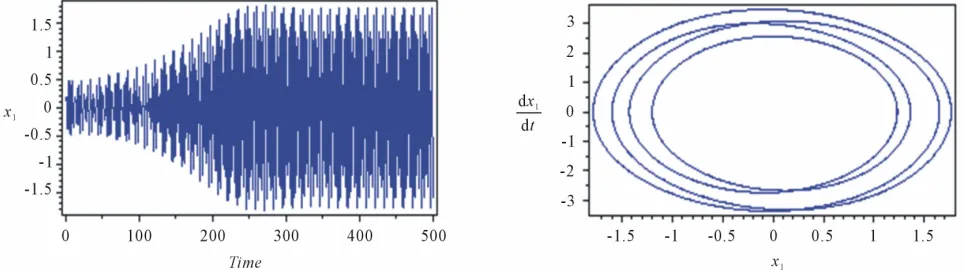
Figure 1 shows the steady state amplitude and phase
plane of the main system at the primary resonance where
11. In this figure, we observe that the steady state
amplitude is about four of the maximum excitation force amplitude F1. The system is stable with multi-limit cycle
and the response of the system is tuned with some chaos.
Figure 2 shows the steady state amplitude and phase
plane of the main system at the sub-harmonic resonance case where 2 21. We note that the steady state
plitude is about 3 of the maximum excitation force am-plitude F1. Also the chaotic wave motion will increase.
The steady state amplitude and phase plane of the main system at simultaneous primary and principle pa-rametric resonance respectively where 11, 2 21
is shown in Figure 3. In this figure, the steady state
plitude is about 5 of the maximum excitation force am-plitude F1 respectively. The system is stable with fine
Table 1. Summary of worst resonance cases.
Cases Conditions Amplitude ratio x F1 1
without absorber
Amplitude ratio x F1 1
with absorber
Amplitude ratio
x F2 1
a
E Remarks
1 2
500% 0.33% 42% 1500 Multi-limit cycle
2 2 1
500% 28% 42% 18 Limit cycle
2 3 1
500% 33% 33% 15 Limit cycle
2 4 1
500% 30% 30% 16 Limit cycle
2 5 1
500% 30% 30% 16 Limit cycle
1 1
2 21
1 2
3 2 500% 21% 30% 23 Limit cycle
Figure 1. System behavior without absorber at 1 1 and 2 is a way from 1. ξ1 = 0.05, α1 = 0.03, α2 = 0.04, F2 = 0.3.
limit cycle, denoting that the system is free from dy-namic chaos.
[image:6.595.60.539.286.413.2]4.1. Effect of the Controller
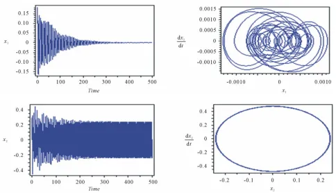
Figure 4 shows that the steady state amplitude of the
system with absorber at the simultaneous resonance 1
1, 2 21 and 2 1. It can be seen for the main
system that the steady state amplitude is 0.33%, but the steady state amplitude of the controller is about 42% of excitation amplitude F1. This means that the
effective-ness of the absorber Ea (Ea = the steady state amplitude
of the main system without absorber/the steady state am-plitude of main system with absorber) is about 1500. Also, the oscillations of the system and absorber have multi-limit cycle and limit cycle respectively.
4.2. Frequency Response Curves
The frequency response Equations (29) and (30), practical case are nonlinear algebraic equations, which are solved numerically. The numerical results are shown in Figures 5-14. These figures, show the steady state response-fre-
quency curve for the stability second case (practical case), where a1, a2 ≠ 0 in the case of simultaneous primary,
sub-harmonic resonance in the presence of one-to-one internal resonance. Figure 5 shows that the effect of the
detuning parameter 1 on the steady state amplitude of
the main system. In this figure, we observe that, the am-plitude a1 has one continuous curve. From this figure, we
observe that the steady state amplitude of the main sys- tem have multi-valued solutions.
[image:6.595.56.540.441.719.2]For increasing excitation forces F1, F2 and for increas-
Figure 3. System behavior without absorber at 11 and 2 21.
ing natural frequencies, we note that the steady state
of the main system and the absorber magnitude of the main system is increased as shown in
Figures 6-8. Figures 9 and 10 show that as non-linear
spring stiffness 3 or 5 are increased positively the
con-tinuous curve is moved downwards and has decreased magnitudes. It can be concluded that increasing the non- linear spring stiffness 3 or 5 can reduce the amplitude
of the system and obtain the effect of reduction of the vibration amplitude. Also for negative value of non-lin- ear spring stiffness 3 or 5 the response amplitude is
[image:7.595.342.507.87.184.2] [image:7.595.341.505.219.318.2]bent to the left and the stability region is decreased.
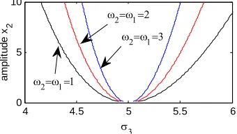
Figure 11, shows that the effects of detuning
parame-ter 3 on the amplitude of the absorber. From this figure,
we observe that the steady state amplitude of the ab-sorber has single-valued solution. From Figures 12-14
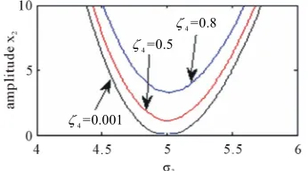
we note that for decreasing natural frequencies or de-creasing non-linear parameter 2 or decreasing linear
damping coefficient 4 the curves diverge down and the
steady state amplitude is decreasing.
5. Conclusions
The system consists
representing the vibration of many applications in ma-chine tools, ultrasonic cutting process, subjected to ex-
-5 0 5
0 5 10 15 20
a
m
pl
it
ud
e x
[image:7.595.338.508.353.445.2]1
Figure 5. Effects of the detuning parameter1.
-5 0 5
0 5 10 15 20
a
m
pl
it
ud
e x
1
f 1=0.6 f 1=20
[image:7.595.98.246.396.474.2]f 1=50
Figure 6. Effects of the excitation amplitude F1.
-5 0 5
0 5 10 15 20
am
pl
it
u
de x
1
f 2=0.3 f
2=20
f 2=50
-2 -1 0 1 2 3
0 5 10 20
Figure 7. Effects of the excitation amplitudeF2.
15
am
pl
it
ude
x1
Figure 8. Effects of the natural frequencies.
-5 0 5
0 5 10 15 20
A
m
pl
it
u
de of
x 1
Figure 9. Effects of the non-linear parameter 3.
-5 0 5
0 5 10 15 20
am
pl
it
ud
e x
1
Figure 10. Effects of the non-linear parameter 5.
4 4.5 5 5.5 6
0 5 10
am
p
lit
ud
e x
[image:7.595.342.503.479.577.2]2
Figure 11. Effects of the detuning parameter 3.
4 4.5 5 5.5 6
0 5 10
am
pl
it
ud
e x
2
[image:7.595.98.250.510.595.2]
[image:7.595.338.508.617.713.2] [image:7.595.96.251.629.714.2]4 4.5 5 5.5 6 0
5 10
am
pl
it
ud
e x
2
Figure 13. Effects of the non-linear parameter 2.
4=0.001
4=0.5
4=0.8
[image:8.595.90.255.85.188.2]
Figure 14. Effects of the damping coefficient 4.
ternal and parametric excitation forces is considered and solved using the method of multiple scale perturbation. A simple and powerful effective method is demonstrated to reduce (control passively) both vibration and dynam chaos in the non-linear system using non-linear absorber One of the most common methods of vibration control is the dynamic absorber. Multiple scales perturbation tech-nique is applied to determine approximate solu the co
lutions and their stability are studied for selected
val-ring; the region of unstable is in-cr
litude of the absorber for increasing va
lued curve which is shifted down-w
the main mass and obtain the ef-fe
erical simulations show the system exhibits pe-rio
[1]
ic .
tions of upled non-linear differential equations. Steady state so
ues of different parameters. Frequency response equa-tions are deduced to investigate system stability. It can be seen from the results that the optimal working conditions of the system is simultaneous primary, sub-harmonic and internal resonance 11, 2 21, 21. From the
above study the following may be concluded.
1) The optimum working conditions for the system are when, 11, 2 21, 21 since the steady state
amplitude of the main system is reduced to 0.33% of its maximum value. This means that the effectiveness of the absorber Ea = 1500.
2) The steady state amplitude is a monotonic increas-ing function to the excitation amplitudes F1, F2 and
natu-ral frequency 1.
3) The zones of multi-valued region are increased for large values of F1.
4) For increasing positive value of non-linear spring stiffness 5 the continuous curve is shifted downwards
produce hard spring.
5) For negative values of 3, the curve is bent to the
left produce soft sp eased.
6) The region of multi-valued is disappeared from the steady state amp
lue of damping coefficient 4, and the continuous
curve has a single-va ards.
7) Increasing the non-linear spring stiffness 5 can
re-duce the amplitude of
ct of reduction of the vibration amplitude, which is a good agreement with Reference [14].
8) Num
dic motions and chaotic motions, which is a good ag- reement with Reference [14].
REFERENCES
S. S. Oueini and A. H. Nayfeh, “Single-Mode Control of a Cantilever Beam under Principal Parametric Excitation,” Journal of Sound and Vibration, Vol. 224, No. 1, 1999, pp. 33-47. doi:10.1006/jsvi.1998.2028
[2] K. R. Asfar, “Effect of Non-Linearities in Elastomeric Material Dampers on Torsional Vibration Control,” In- ternational Journal of Non-Linear Mechanics, Vol. 27, No. 6, 1992, pp. 947-954.
doi:10.1016/0020-7462(92)90047-B
[3] M. Eissa, “Vi Linear Mechanical
Systems via Neutra neering Bulle-
abad, 2000.
l. 66, bration Control of
Non-lizers,” Electronic Engi tin, No. 18, 1999.
[4] M. Eissa, “Vibration and Chaos Control in I.C Engines Subject to Harmonic Torque via Non-Linear Absorbers,” Proceedings of ISMV Conference,Islam
[5] M. Eissa and W. El-Ganaini, “Part I, Multi-Absorbers for Vibration Control of Non-Linear Structures to Harmonic Excitations,” Proceedings of ISMV Conference, Islama-bad, 2000.
[6] M. Eissa and W. El-Ganaini, “Part II, Multi-Absorbers for Vibration Control of Non-Linear Structures to Harmonic Excitations,” Proceedings of ISMV Conference, Islama-bad, 2000.
[7] M. M. Kamel and Y. A. Amer, “Response of Parametri-cally Excited One-Degree-of-Freedom System with Non- Linear Damping and Stiffness,” Physica Scripta, Vo No. 6, 2002, pp. 410-416.
doi:10.1238/Physica.Regular.066a00410
[8] Y. Song, H. Sato, Y. Iwata and T. Komatsuzaki, “The Response of a Dynamic Vibration Absorber System with a Parametrically Excited Pendulum,” Journal of Sound and Vibration, Vol. 259, No. 4, 2003, pp. 747-759. doi:10.1006/jsvi.2002.5112
[9] A. Soom and M. Lee, “Optimal Design of Linear and Non- Linear Vibration Absorbers for Damped System,” Jour- nal of Vibration, Acoustic Stress, and Reliability in De- sign, Vol. 105, No. 4, 1983, pp. 112-119.
doi:10.1115/1.3269054
[image:8.595.86.259.223.319.2]al of Sound and Vibration [11] H. J. Rice, “Combinational Instability of the Non-Li
Vibration Absorber,” Journ
near , Vol. 108, No. 4, 1986, pp. 526-532.
doi:10.1016/S0022-460X(86)80046-3
[12] J. Shaw, S. W. Shaw and A. G. Haddow, “On the Re- sponse of the Non-Linear Vibration Absor
tional Journal of Non-L
ber,” Interna-inear Mechanics, Vol. 24, No. 4, 1989, pp. 281-293. doi:10.1016/0020-7462(89)90046-2 [13] S. Natsiavas, “Steady State Oscillations and Stability of
Non-Linear Dynamic Vibration Absorbers,” Journal of Sound and Vibration, Vol. 156, No. 2, 1992, pp. 227-245. doi:10.1016/0022-460X(92)90695-T
[14] S. J. Zhu, Y. F. Zheng and Y. M. Fu, “Analysis of Non- Linear Dynamics of a Two-Degree-of
System with Non-Linear Damping and N-Freedom Vibrationon-Linear Spring,” Journal of Sound and Vibration, Vol. 271, No. 1-2, 2004, pp. 15-24. doi:10.1016/S0022-460X(03)00249-9
[15] A. H. Nayfeh, “Resolving Controversies in the Applica-tion of the Method of Multiple Scales and the Generalized Method of Averaging,” Nonlinear Dynamics, Vol. 40, No. 1, 2005, pp. 61-102. doi:10.1007/s11071-005-3937-y [16] Y. A. Amer, “Vibration Control of Ultrasonic Cutting via
Dynamic Absorber,” Chaos, Solutions and Fractals, Vol. 33, No. 5, 2007, pp. 1703-1710.
doi:10.1016/j.chaos.2006.03.038
[17] M. Eissa and M. Sayed, “A Comparison between Passive and Active Control of Non-Linear Simple Pendulum Part-I,” Mathematical and Computational Applications, Vol. 11,
11,
m,” Communication in l Simulation, Vol. 13, No. 2, 2006, pp. 137-149.
[18] M. Eissa and M. Sayed, “A Comparison between Passive and Active control of Non-Linear Simple Pendulum Part-II,” Mathematical and Computational Applications Vol. No. 2, 2006, pp. 151-162.
[19] M. Eissa and M. Sayed, “Vibration Reduction of a Three DOF Non-Linear Spring Pendulu
Nonlinear Science and Numerica No. 2, 2008, pp. 465-488. doi:10.1016/j.cnsns.2006.04.001
[20] M. Sayed, “Improving the Mathematical Solutions of Nonlinear Differential Equations Using Different Control Methods,” Ph.D. Thesis, Menofia University, Shebin El- Koom, 2006.
[21] Y. S. Hamed, W. El-Ganaini and M. M. Kamel, “Vibra-
i:10.1007/s12206-009-1208-9
tion Suppression in Ultrasonic Machining Described by Non-Linear Differential Equations,” Journal of Mecha- nical Science and Technology, Vol. 23, No. 8, 2009, pp. 2038-2050. do
[22] Y. S. Hamed, W. El-Ganaini and M. M. Kamel, “Vibra- tion Suppression in Multitool Ultrasonic Machining to Multi-External and Parametric Excitations,” Acta Mecha- nica Sinica, Vol. 25, No. 3, 2009, pp. 403-415.
doi:10.1007/s10409-009-0229-7
[23] Y. S. Hamed, W. El-Ganaini and M. M. Kamel, “Vibra- tion Reduction in Ultrasonic Machine to External and Tuned Excitation Forces,” Applied Mathematical Model- ling, Vol. 33, No. 6, 2009, pp. 2853-2863.
doi:10.1016/j.apm.2008.08.020
[24] M. Sayed and Y. S. Hamed, “Stability and Response of a Nonlinear Coupled Pitch-Roll Ship Model under Para-metric and Harmonic Excitations,” Nonlinear Dynamics, Vol. 64, No. 3, 2011, pp. 207-220.
doi:10.1007/s11071-010-9841-0
[25] M. Sayed and M. Kamel, “Stability Study and Control of Helicopter Blade Flapping Vibrations,” Applied Mathe- matical Modelling, Vol. 35, No. 6, 2011, pp. 2820-2837. doi:10.1016/j.apm.2010.12.002
[26] M. Sayed and M. Kamel, “1:2 and 1:3 Internal Resonance Active Absorber for Non-Linear Vibrating System,” Ap- plied Mathematical Modelling, Vol. 36, No. 1, 2012, pp. 310-332. doi:10.1016/j.apm.2011.05.057
[27] Y. A. Amer and M. Sayed, “Stability at Principal Reso-
n Techniques,” nance of Multi-Parametrically and Externally Excited Me- chanical System,” Advances in Theoretical and Applied Mechanics, Vol. 4, No. 1, 2011, pp. 1-14.