Model for Solving Fuzzy Multiple Objective Problem

Model for Solving Fuzzy Multiple Objective Problem

Ritika Chopra1, Ratnesh R. Saxena2

1

Department of Mathematics, Delhi University, Delhi, India

2

Department of Mathematics, Deen Dayal Upadhyay College, Delhi University, Delhi, India Email: [email protected]

Received November 27, 2012; revised December 25, 2012; accepted January 10, 2013

ABSTRACT

In real world decision making problems, the decision maker has to often optimize more than one objective, which might be conflicting in nature. Also, it is not always possible to find the exact values of the input data and related parameters due to incomplete or unavailable information. This work aims at developing a model that solves a multi objective dis-tribution programming problem involving imprecise available supply, forecast demand, budget and unit cost/profit co-efficients with triangular possibility distributions. This algorithm aims to simultaneously minimize cost and maximize profit with reference to available supply constraint at each source, forecast demand constraint at each destination and budget constraint. An example is given to demonstrate the functioning of this algorithm.

Keywords: Decision Making Problems;Multi Objective Distribution Programming Problem; Fuzzy Set Theory

1. Introduction

The distribution planning decision (DPD) problem in- volves optimizing the distribution plan for transporting goods from a set of sources to a set of destinations in a supply chain. With a variety of distributing routes, the aim of the DPD problem is to determine how many units should be shipped from one source to one destination so that the available supply at each source and the forecast demand at each destination are satisfied. In most real- world DPD problems, the decision maker (DM) must simultaneously handle conflicting objectives like mini- mizing total distribution costs, number of rejected items and delivery time/distance, and maximizing total profits, relative safety and customer service level.

When any of the ordinary linear programming (LP) method or the existing solution algorithms is used to solve DPD problems, the objectives and model inputs are generally assumed to be precisely given (crisp). However, in practical DPD problems, input data and related pa- rameters, such as available supply, forecast demand and related cost/time/profit coefficients, are often imprecise (fuzzy) because of incomplete or (and) unavailable in- formation. So, conventional LP method and solution al- gorithms cannot solve the imprecise (fuzzy) DPD pro- gramming problems.

Fuzzy set theory was presented by Zadeh [1] and has been applied extensively in various fields. His study showed that the importance of the theory of possibility is based on the fact that much of the information, on which human decisions are based, is possibilistic rather than

probabilistic in nature. In 1976, Zimmermann [2] first introduced fuzzy set theory into an ordinary LP problem with fuzzy objective and constraints. Following, the fuzzy decision making method proposed by Bellman and Zadeh [3] confirmed the existence of an equivalent ordi- nary LP form. Subsequently, Chanas et al. [4]presented a fuzzy linear programming (FLP) method to solve DPD problems with crisp cost coefficients and fuzzy supply and demand. Furthermore, Zimmermann [5] extended his FLP method to a multi-objective linear programming (MOLP) problem. In addition, researchers have devel- oped several FGP methods to solve multi-objective DPD problems. Li and Lai [6] designed a fuzzy compromise programming method to obtain a non-dominated com- promise solution for multi-objective DPD problems in which various objectives were synthetically considered with the marginal evaluation for individual objectives and the global evaluation for all objectives. Related studies on solving DPD problems with multiple fuzzy objectives included Hussein [7] and Abd El-Wahed [8]. Moreover, Lai and Hwang [9] developed an auxiliary MOLP model for solving PLP problems with imprecise objective and/or constraint coefficients with triangular distributions. Tien-Fu Liang [10] integrated the available concepts to solve multi-objective DPD problems involveing impre- cise available supply, forecast demand and unit cost/time coefficients with triangular possibility distributions.

tions. Also, the interactive PLP method provides a sys- tematic framework that facilitates the decision making process, enabling a DM to interactively modify the im- precise data and related parameters until a satisfactory solution is obtained. The proposed methodology can be applied to various real world multi objective problems such as assignment problems, transportation problems and many more such problems in which the information is given in the form of triangular possibility distributions.

2. Problem Description

A general multi objective distribution programming problem aims to determine the right plan for distributing a homogeneous commodity from m sources to n destina-tions. Each source has an available supply of the com-modity to distribute to various destinations, and each destination has a forecast demand of the commodity to be received from various sources. The available supply for each source, the forecast demand for each destination, and related cost/profit coefficients are generally impre-cise over the planning horizon due to incomplete and/or unobtainable information. The proposed PLP method aims to simultaneously minimize the total distribution costs and maximize the total profit with reference to available supply constraint at each source, forecast de-mand constraint at each destination and the total budget constraint. This work focuses on developing an interac-tive PLP method for optimizing the distribution plan in uncertain environments.

Thus, all the objectives are imprecise thereby incorpo-rating the variations in the decision maker’s judgments relating to the solutions of the multi objective optimiza-tion problems in a framework of fuzzy aspiraoptimiza-tion levels. The pattern of triangular possibility distribution is adopted to represent the imprecise objective functions and related imprecise numbers. All of the objective functions and the constraints are linear and the cost and profit on a given route are directly proportional to the units distributed.

3. Notations

3.1. Index Sets

 i index for source, for all i1, 2,,m;  j index for destination, for all j1, 2,,n;  g index for objectives, for g1, 2.

3.2. Decision Variables

 x_ij units distributed from source i to destination j (units).

3.4. Parameters

 c_ij distribution cost per unit delivered from source i to destination j ($/unit);

 p_ij profit per unit delivered from source i to destina-tion j ($/unit);

 S_i total available supply for each source i (units);  D_j total forecast demand of each destination j

(units);

 B total budget ($).

4. Problem at a Glance

The aim of the problem is to minimize total cost of dis-tribution and maximize profit (where cost and profit co-efficients are fuzzy numbers with triangular possibility distributions) with reference to imprecise available sup-ply constraint at each source, forecast demand constraint at each destination and the total budget constraint. Mathematically,

 

1 1 1 min

m n ij ij i j

z c x

 





(4.1)

 

2 1 1 max

m n ij ij i j

z p x

 





(4.2) Subject to



1

, 1, 2, , n

ij i j

x S i m



  







1

, 1, 2, , m

ij j i

(4.3)

x D j n



  







1 1

0,

1, 2, , , 1, 2, , n m

ij ij ij j i

c x Bx

i m j n

 

 

   





 

(4.4)

(4.5)

5. Methodology

This work assumes the DM to have already adopted the pattern of triangular possibility distribution for all impre-cise numbers. For instance, the triangular possibility dis-tribution of imprecise cost coefficient (given in Figure



 o_, m_, p



ij ij ij ij

c  c c c m

ij

c

o

, where is the most possible 1),

value that definitely belongs to the set of available values (degree of association = 1, if normalized), cij is the

most optimistic value that has a very low likelihood of belonging to the set of available values (degree of asso-ciation = 0) and ijp is the most pessimistic value that

has a very low likelihood of belonging to the set of available values (degree of association = 0).

1

0

o ij

c m

ij

c

1

II 0

p m _Z

Z

p o

ij

c Zg g g

I





13 1 1 min

m n

p m ij ij ij i j

z c c x

 







21 1 1 max

m n m ij ij i j

z p x

 









22 1 1 min

m n

m p ij ij ij i j

z p p x

 











23 1 1 max

m n

o m ij ij ij i j

z p p x

 

[image:3.595.334.536.80.385.2]







Figure 1. Triangular possibility distribution of cij.



Similarly, triangular possibility distribution of impre- cise profit coefficient,pij  pijp,p pijm, ijo



m ij

p

o

p

, where is the most possible value that definitely belongs to the set of available values ( degree of association = 1, if nor-malized), ij is the most optimistic value that has a

very low likelihood of belonging to the set of available values ( degree of association = 0) and ijp is the most

pessimistic value that has a very low likelihood of be-longing to the set of available values ( degree of associa-tion = 0).

p

Geometrically, these imprecise objective functions are fully defined by three prominent points

   

zm,1 , zo, 0



and zp, 0



m

z



_zm_zo



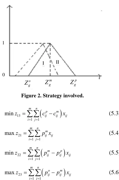
. The imprecise cost objective can be mini-mized by pushing the three prominent points of triangu-lar possibility distribution towards left and the imprecise profit objective can be maximized by pushing these points to the right. Because of the vertical coordinates of the prominent points being fixed at either 1 or 0, the three horizontal coordinates are the only considerations. Thus we aim to simultaneously minimize the most possi-ble objective value of the imprecise cost objective func-tion, 1 , maximize the possibility of obtaining lower

objective value, 1 1 (region I of the possibility

distribution in Figure 2), and minimize the risk of ob-taining higher objective value,





1 1

p m

z z



2 2



m p

z z

(region II of the possibility distribution in Figure 2) and maximize the most possible objective value of the imprecise profit ob-jective function, 2 , minimize the possibility of

obtain-ing lower objective value, (i.e. region I) and maximize the possibility of obtaining higher objective value, (i.e. region II).

m

z





_zo_z

2 2

Therefore, the above two fuzzy objectives are broken down into the following six crisp objectives

m

11 min

1 1

n m m ij ij j i

z c x

 









1 1

m o ij ij ij

c c x

(5.1)

12 max

m n i j

z

 

[image:3.595.91.264.80.231.2]





(5.2)

Figure 2. Strategy involved.

(5.3)

(5.4)

(5.5)

(5.6) _,

i

S at each Further, the imprecise available supply

 source and the imprecise forecast demand, Dj



S

, at each destination have triangular possibility distributions with the most and least possible values. _i and D_jare con-verted to crisp numbers by applying the weighted sum approach. Let the minimum acceptable possibility, , be given by the DM. Then the corresponding auxiliary inequality constraints can be represented as follows

1 , 2 , 3 ,

1

1,

, 2, ,

n

o m p

ij i i i j

x w S _ w S _ w S _ i m



    





1 , 2 , 3 ,

1

1, 2, , ,

m

o m p

ij i i i i

(5.7)

x w D _ w D_ w D _ j n



    





1

w w w

(5.8)

where, 1 2 3 , w w1, 2andw3 represent the

weights of the most possible values, most optimistic val-ues and the most pessimistic valval-ues of the imprecise sup-ply demand, respectively. Related methods and algo-rithms for determining weights include the analytic hier-archy process (AHP) and direct assessment methods. In real-world DPD problems, detailed study of the effects of various weighting methods should be based on a DM’s experience and knowledge.

1 1

i j

1 1

m n

o o ij ij i j

c x B



   



1 1 m n p p ij ij i j

c x B

(5.10)    

















1 1 2 2 1 1 2 2 ax , in , in , ax , m o m p m o m p z z z z z z z z z    



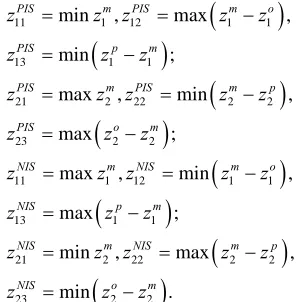
(5.11)

The auxiliary MOLP problem developed above can be converted into an equivalent ordinary LP form using Zimmermann’s linear membership functions [2] to rep-resent all of the fuzzy objectives of the DM, together with the fuzzy decision-making concept of Bellman and Zadeh [3]. First, obtain the corresponding positive ideal solutions (PIS) and negative ideal solutions (NIS) of all the crisp objective functions of the auxiliary MOLP problem, as follows

















11 1 12

13 1 1

21 2 22

23 2 2

11 1 12

13 1 1

21 2 22

23 2 2

min m min ; max m max ; max m max ; min m , , in . , m , PIS m PIS PIS p m PIS m PIS PIS o m NIS m NIS NIS p m NIS m NIS NIS o m

z z z

z z z

z z z

z z z

z z z

z z

z z z

z z z

               

Furthermore, the corresponding linear membership function for each of the new objective functions of the auxiliary MOLP problem is defined by

 

11

11 11

11 11 11

11 11 11 1 i if 0 i NIS 11 11 11 11 f f PIS PIS NIS PIS NI

z z NIS

S z z f z z z       _   

z z z

z z     (5.12) 12 12

0 if zNIS z

 _



Linear membership functions for objective functions (5.3) and (5.5) are similar to the linear membership func-tion for objective funcfunc-tion (5.1) given by the Equafunc-tion (5.12) and the linear membership function for objective functions (5.4) and (5.5) are similar to the linear mem-bership function for objective function (5.2) given by the Equation (5.13).

Finally, aggregate all fuzzy sets using the minimum operator of fuzzy decision making concept. Let λ be the



0 1



, which represents the de- auxiliary variable 

gree of satisfaction of the decision maker. Then, the cor-responding single objective linear programming problem is max λ

 

 

 

1 1 2 2

3 3

1 , 2 , 3 ,

1

1 , 2 , 3 ,

1

1 1 1 1 1 1

, 1, 2; , 1, 2;

, 1, 2

, 1, 2, ,

1, 2, ,

, ,

s.t

,

g g g g g g

n

o m p ij i i i j

m

o m p ij i i i i

m n m n m n

m m o o p p ij ij ij ij ij ij i j i j i j

f z g f z g

f z g

x w S w S w S i m

x w D w D w D j n

c x B c x B c x B

                                      











  ,

0, 1, 2, , , 1, 2, , .

ij

x   i  m j   n

The above problem is a crisp single objective linear programming problem which can easily be solved using MATLAB.

6. Numerical Illustration

[image:4.595.97.246.322.473.2]

Consider the problem given in Table 1. Also, the total budget,

Table 1. Problem in consideration.

A B C D Supply (in thousand)

1 (0.6,0.8,0.9)

* (0.1,0.3,0.4)** (2.4,3.0,3.5) (1.0,1.5,2.0) (1.8,2.1,2.3) (1.0,1.4,1.6) (1.5,1.8,2.0) (0.7,0.9,1.0) (17.2,18.0,19.2)

2 (1.1,1.3,1.4)

(0.4,0.6,0.7) (3.1,3.6,4.1) (1.5,1.8,2.1) (1.4,1.6,1.7) (0.8,0.9,1.1) (2.2,2.5,2.7) (1.0,1.4,1.8) (22.6,24.0,25.8)

3 (1.5,1.8,2.0)

(0.6,0.9,1.1) (3.1,3.5,3.9) (1.4,1.8,2.2) (2.1,2.4,2.7) (1.3,1.5,1.7) (0.8,1.0,1.1) (0.2,0.3,0.4) (12.6,13.0,13.6)

Demand in thousand (11.2,12.0,12.6) (5.4,6.0,6.4) (14.8,16.0,16.8) (19.0,20.0,20.8)

*





$ 132000,14

B _{0000,148000 .}

First, formulate the original multi-objective fuzzy problem using Equations (4.1) to (4.5). Then, develop the new objective functions for the new crisp multi-objective problem using Equations (5.1) to (5.6). Further, defuzzify fuzzy constraints to get crisp constraints using Equations (5.7) to (5.11) at  0.5 assuming w1w31 4 and

2

w

14 24 34

06957 00001; 13018 ;

x x x



 

; 1 2

 .

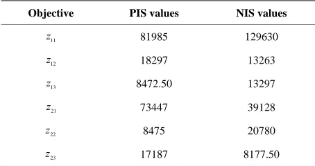
Get the PIS and NIS values (given in Table 2 below) corresponding to all the crisp objectives.

Additionally, the corresponding linear membership function for each of the fuzzy objectives in the auxiliary MOLP can be defined using Equations (5.12) and (5.13). Finally, the auxiliary MOLP can be converted to an equivalent LP model using the minimum operator to ag-gregate all fuzzy sets. This LP is then solved using MATLAB.

The solutions are imprecise and have triangular possi-bility distribution, and overall degree of decision maker satisfaction is 0.9861. Thus, the optimal plan by the above method is as follows:



_

_

11 12 13

21 22 23

31 32 33

11 12 13

1

21 22 23

10211, 00667, 00002, 01764, 05304, 15948, 00001, 00004, 00001, 82640, 13331, 8473.70

, , . ;

39203, 8611, 8

x x x

x x x

x x x

z z z

z

z z z

   

  

 

  



  

69309 82640 91113 70



_

_

2

312.10

, , . ;

z  30592 39203 47515 10

;

;

7. Conclusions

[image:5.595.58.285.581.701.2]

This work develops an interactive method for solving multi-objective problems with imprecise available supply, forecast demand and unit cost/profit coefficients with triangular possibility distributions. The model designed here aims to simultaneously minimize the total distribu-

Table 2. PIS and NIS values of the objectives.

Objective PIS values NIS values

11

z 81985 129630

18297 13263

8472.50 13297

73447 39128

8475 20780

17187 8177.50

tion costs and maximize the total profit with reference to available supply at each source, as well as forecast de-mand constraints at each destination and the total budget constraint.

The method developed can be easily applied to any real world problem with triangular distributions such as distribution planning decision problems, assignment problems, job allocation problem and more such prob-lems. It provides a systematic framework that facilitates the decision-making process, enabling a DM to interac-tively modify the imprecise data and related parameters until a set of satisfactory solutions is obtained.

REFERENCES

[1] L. A. Zadeh, “Fuzzy Sets as a Basis for a Theory of Pos-sibility,” Fuzzy Sets and Systems, Vol. 1, No. 1, 1978, pp. 3-28. doi:10.1016/0165-0114(78)90029-5

[2] H.-J. Zimmermann, “Description and Optimization of Fuzzy Systems,” International Journal of General Sys-tems, Vol. 2, No. 1, 1976, pp. 209-215.

doi:10.1080/03081077508960870

[3] R. E. Bellman and L. A. Zadeh, “Decision-Making in a Fuzzy Environment,” Management Science, Vol. 17, No. 4, 1970, pp. 141-164.

[4] S. Chanas, W. Kolodziejczyk and A. Machaj, “A Fuzzy Approach to the Transportation Problem,” Fuzzy Sets and Systems, Vol. 13, No. 3, 1984, pp. 211-222.

doi:10.1016/0165-0114(84)90057-5

[5] H.-J. Zimmermann, “Fuzzy Programming and Linear Programming with Several Objective Functions,” Fuzzy Sets and Systems, Vol. 1, No. 1, 1978, pp. 45-56. doi:10.1016/0165-0114(78)90031-3

[6] L. Li and K. K. Lai, “A Fuzzy Approach to the Multi- Objective Transportation Problem,” Computers and Op-erations Research, Vol. 27, No. 1, 2000, pp. 43-57. doi:10.1016/S0305-0548(99)00007-6

[7] M. L. Hussein, “Complete Solutions of Multiple Objec-tive Transportation Problems with Possibilistic Coeffi-cients,” Fuzzy Sets and Systems, Vol. 93, No. 3, 1998, pp. 293-299. doi:10.1016/S0165-0114(96)00216-3

[8] W. F. Abd El-Washed, “A Multi-Objective Transporta-tion Problem under Fuzziness,” Fuzzy Sets and Systems, Vol. 117, No. 1, 2001, pp. 27-33.

doi:10.1016/S0165-0114(98)00155-9

[9] Y. J. Lai, and C. L. Hwang, “A New Approach to Some Possibilistic Linear Programming Problem,” Fuzzy Sets and Systems, Vol. 49, No. 2, 1992, pp. 121-133.

doi:10.1016/0165-0114(92)90318-X

12

z

13

z

21

z

22

z

23

z

[10] T. F. Liang, “Application of Possibilistic Linear Pro-gramming to Multi-Objective Distribution Planning De-cisions” Journal of the Chinese Institute of Industrial En-gineers, Vol. 24, No. 2, 2007, pp. 97-109.