D S Sharma, R Sangal and E Sherly. Proc. of the 12th Intl. Conference on Natural Language Processing, pages 39–48, Trivandrum, India. December 2015. c2015 NLP Association of India (NLPAI)
Self-Organizing Maps for Classification of a Multi-Labeled Corpus
Lars Bungum and Bj¨orn Gamb¨ack Department of Computer and Information Science
Norwegian University of Science and Technology Sem Sælands vei 7–9, 7094 Trondheim, Norway
{larsbun,gamback}@idi.ntnu.no
Abstract
A Self-Organizing Map was used to clas-sify the Reuters Corpus, by assigning a la-bel to each of the documents that cluster to a specific node in the Self-Organizing Map. The predicted label is based on the most frequent label among the train-ing documents attributed to that particu-lar node. Experiments were carried out on different grid sizes (node numbers) to de-termine their influence on classification sults. Informative visualizations of the re-sulting Self-Organizing Maps are demon-strated. We argue that the Self-Organizing Map is well suited to classify a document collection in which many documents si-multaneously belong to several categories.
1 Introduction
Categorization of a text corpus in which each arti-cle is attributed with a set of categories (labels), is a classicalsupervisedclassification task. Most su-pervised classification methods learn parameters from a training set of labeled instances, and use the learned model to score test instances. The Self-Organizing Map (SOM) is in contrast an un-supervised technique, clustering similar training instances together, without knowledge of their cat-egories. The resulting maps display visually iden-tifiable, but non-delimited, clusters. In this way, the SOM algorithm makes underlying similarities in high-dimensional space visible in lower dimen-sions. Through a two-step methodology, the la-bels of a training corpus associate with areas of the map; areas that in turn can be used to classify previously unseen documents.
The Reuters Corpus (Lewis et al., 2004) con-sists of text documents with a varying amount of labels attributed to them. Sebastiani (2002) notes a fundamental distinction between thesingle-label
and multi-label classification tasks. In the for-mer, only one label is attributed to each docu-ment, whereas any number can be attributed to the documents in the latter. Most research has gone into the single-label problem, as this will gener-alize to multi-label classification, by transforming the problem to a sequence of binary classification problems. This however, rests on the assumption that the categories are stochastically independent, that is, that the label of a document does not de-pend on the whether the document also has an-other label.
Another key problem in document classification relates to vectorization, how a group of documents is converted into a vector-based feature representa-tion. The way documents are represented, and of-ten the cut-off point in deriving TFIDF or ngram statistics, will result in different amounts of fea-tures. Documents can in principle be vectorized to any dimensionality, in its simplest form counts of occurrences of a given set of words.
A number of experiments were conducted on two different portions of the Reuters Corpus, the Top 10 and Full set of categories, respectively. While this follows a tradition of SOM-based clas-sification, we offer more details on the implemen-tation, the vectorization, and the parameters for creating the map. Self-Organizing Maps of dif-ferent sizes were used to evaluate the importance of the number of nodes in SOM classification. The cost of computing the maps increase with the size of their topologies, posing the research question: Can this be justified with classifier performance?
We demonstrate that the method elucidates sim-ilarities between labels as well as between docu-ments, and argue that the reduction of the multi-label classification of the corpus into a cascade of binary classification problems under the assump-tion that the categories are stochastically indepen-dent is not plausible.
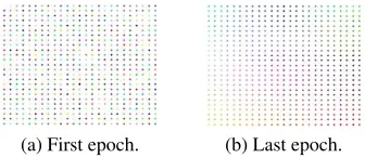
(a) First epoch. (b) Last epoch.
Figure 1: RGB color coding of a SOM.
Section 2 discusses related work and presents some background on the SOM algorithm and us-ing them as a classification device, while Sec-tion 3 describes the Reuters Corpus and SecSec-tion 4 goes through the applied methodology. Section 5 presents the experimental results, that are further discussed in Section 6. Section 7 concludes and looks forward.
2 Self-Organizing Maps
Self-Organizing Maps (Kohonen, 1982) is a Clus-ter Analysis Algorithm with roots in Artificial Neural Networks, also termed Kohonen Neural Networks, as discussed by Lo et al. (1991). A SOM functions on nodes organized according to a given topology (usually 2-dimensional). The nodes are made up by vectors of some higher di-mensionality, directly comparable to vectors rep-resenting training samples. The properties of the nodes are gradually changed during a pre-defined number of epochs, making the nodes more similar to the training samples. Changing one data point (node) will also affect its neighboring nodes, in a fashion inspired by biological systems in which neurons with similar functions organize in the same areas.
This process is illustrated in Figure 1, where 25x25 nodes are represented as vectors with three dimensions, each with values between 0 and 1. The training samples consist of a set of fixed col-ors, encoded as RGB (red, green, and blue) val-ues. After the end of training, the grid has “self-organized“ into areas of similar colors. This is accomplished by comparing each training sample to each node, according to adistance metric, and drawing the closest node (“the winner”) and its neighborhood towards the training sample. The samples are processed serially, and this is repeated fornepochs, as outlined in Figure 2.
Samples can be of any dimensionality; the higher the dimensionality, the more computation-ally costly will each comparison be. The result-ing map will group (self-organize) similar
high-1. Initialize nodes in the 2-dimensional topology. 2. (a) Sample all vectorized documents from the
training material in succession.
(b) Find the closest match in the node layout. (c) Update this matching node and its
neigh-bors to be closer to the sample.
3. Reduce learning rate and/or neighborhood size. 4. Return to Step 2 until end of all epochs.
Figure 2: SOM algorithm.
dimensional vectors together, that can be visu-ally inspected in the original topology, a low-dimensional space. Hence a feat of cartography in the landscape of documents is achieved, not only because documents are found in the same areas on the map, but also because the distances between nodes are visible with color shadings or contour plots. In this way differences in high-dimensional space become apparent in lower dimensions, cre-ating a dimensionality reduction.
Hy¨otyniemi (1996) used a SOM to extract fea-tures for document representation, based on the clustering of character trigrams, arguing that this would account better for linguistic features.
Eyassu and Gamb¨ack (2005) and Asker et al. (2009) used Self-Organizing Maps to classify Amharic news text. Categorized by experts, each document in the training corpus was associated with a query. A merged query and document ma-trix (i. e., the vector representation of the collec-tion) was used for training the SOM. They report using many epochs (up to 20,000) and achieved classification accuracies in line with comparable methods such as Latent Semantic Indexing (Deer-wester et al., 1990).
In order to use the SOM for a supervised classi-fication task, consisting of a training and test cor-pus, it is necessary to establish a mechanism by which to ascribe a label to each of the test sam-ples, i. e., what class membership (label) topredict for the sample in question. During classification, a test sample will be compared to the 2-dimensional grid to find itswinning node, just like in training.
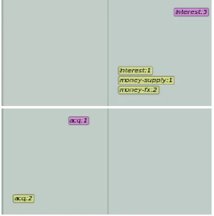
Figure 3: Example of SOM clustering with ma-jority voting. Yellow labels from training corpus, magenta labels from test corpus.
by majority vote of the class labels of all train-ing samples that had this node as winner. In the last run of the SOM, the Best-Matching Unit (BMU) of each training sample in the final epoch is recorded.
For empty nodes, being no sample’s BMU, the next closestn nodes (the BMUs being the clos-est) are investigated for training samples until a non-empty node is found. The prediction is made according to the most frequent label of this node.
This process is illustrated with Figure 3, where each square represents a node (so a 2x2 SOM). Two of the four nodes have documents attaching to them. The yellow labels are from the training corpus, and the magenta from test samples. The SOM classifies test documents correctly, if their labels match that attributed to them by the node.
In the bottom-left node, both matching training samples (2 in yellow) had the labelacq (acquisi-tions), which would be the prediction of this node. The one test sample (1 in magenta) that had this node as its BMU was also labeledacq, i. e., a cor-rect prediction.
For the top-right node, the figure shows that the four training samples were split between money-fx(2), money-supply(1) andinterest (1). By ma-jority voting, the predicted label of the node be-comesmoney-fx. However, the five test samples were all labeled interest, and all of them would thus be falsely classified (asmoney-fx).
3 Data
The Reuters Corpus (Lewis et al., 2004) has been used extensively for text classification research. For easier comparison of results, several ways of processing the corpus have been established. Those pertain to the corpus subsets, and a spe-cific split of it into training and test sets called the
ModApt´esplit (Lewis, 1997).
A further much used split means dividing the
ModApt´e into either the ten most frequent cat-egories, the categories with at least one positive training and one test example (90), or the cate-gories with at least one training example (115).
The split with the 90 categories with at least one positive training and test example is some-what confusingly called Apt´eMod by Yang and Liu (1999), while Debole and Sebastiani (2004) refer to it as the R(90) subset of the ModApt´e
split. Elsewhere, the R(90) split with 10,789 docu-ments is also calledModApt´e(Yang et al., 2009; Chen et al., 2004; Saarikoski et al., 2011).
The Natural Language Toolkit (NLTK) in-terface (Loper and Bird, 2002) to the Reuters Corpus provides the Apt´eMod split as com-prised by 7,769 training examples and 3,019 test instances. The category frequencies are
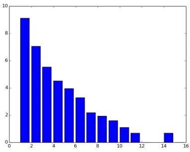
[9160,1173,255,91,52,27,9,7,5,3,2,1,0,2,1],
i. e., 9,160 documents with just one category, 1,173 with two, etc. A plot of the log-frequency of categories is shown in Figure 4.
The NLTK interface provides a data structure where the raw text and categories are indexed on filenames. This was used in the present work, and the documents were transformed into a matrix of TF-IDF values, i. e., the product of the Term Fre-quency (the occurrence of the term in the docu-ment) and the Inverse Document Frequency (the log of the number of documents containing this term). A term can be any n-gram.
The corpus is comprised of text documents with 0 to 15 different category labels. The five most frequent labels of the 90 categories in the ModApt´e split have the following counts:
[3923,2292,374,326,309], totalling 7,224 of the
9,160 documents. The skewed distribution means that accuracy on the entire corpus is not al-ways a good measure of classifier performance, as the performance on less frequent categories may drown in the larger categories. The distinction be-tween micro- and macroaveraging mitigates this.
Figure 4: Log-frequencies of categories in the Reuters Corpus. Log of 0 set to 0.
to be classified within an experiment counting all correct predictions in one pool and dividing by the number of classified documents. This is expressed in Equation 1 wherecdenotes the number of
cor-rectly classified documents andnthe total number of documents.
Microaverage = c
n (1)
This measure will be skewed towards larger classes: Consider a classifier that classifies one large category with 90 documents 100% correctly, whereas 10 other classes with one document each were all wrong. That would give a microaverage of 90%, even though most categories were com-pletely wrong.
Themacroaverageis a measure that is weighted with relative size, expressed formally in Equa-tion 2 wherecjandnj are the number of correctly
classified documents belonging to classjand the
total number of documents in that class, resp.
Macroaverage =
P cj nj
|Classes| (2) In the same way as for accuracy, micro- and macroaverages can be calculated for precision, re-call and F-score. However, when the classification problem is framed as aone-of classification, i. e., when all documents in the test set belong to ex-actly one class, the microaveraged F-score will be the same as the accuracy, because the number of false positives and false negatives will always be the same. If a document is classified with a label it does not have, it will be a false positive in that class, but also a false negative in the class it cor-rectly belongs to (Manning et al., 2008).
4 Implementation
The Self-Organizing Map algorithm was imple-mented in MPI (mpi4py)1 and Python, and run on a Portable Batch System (PBS)2 scheduler. A quadratic layout of nodes was used for the exper-iments. Samples were processed serially, but for each sample, the vector comparisons and updating of nodes were done in parallel. The availability of large-scale High-Performance Computing (HPC), facilitated feasibility of the “on-line” version of the SOM algorithm. “On-line” as weights are up-dated after processing of each training sample, as formulated in Figure 2.
Methods for reducing computational cost in-clude using a two-step approach (i. e., a SOM on the output of another SOM) (Kohonen et al., 1996), or formulating a “batch-SOM” algorithm. These methods contrast the “on-line” version by updating all node weights in one operation per epoch. See Lawrence et al. (1999) and Patel et al. (2015) for parallel batch-SOM implementations. Fort et al. (2002) compared the approaches and noted some problems with the batch formulation, e. g., initialization sensitivity, while it had advan-tages in terms of speed and efficiency.
In the on-line formulation, vector comparisons and updates are run per training sample, increas-ing linearly with the number of trainincreas-ing samples. In turn, the vector comparisons increase with the number of nodes in the grid. Vector comparisons are costly, and therefore lend themselves well to parallelization. Hence, the parallel on-line imple-mentation used in these experiments is sensitive to a large amount of training samples, but well equipped to handle large SOM topologies.
Each experiment in Section 5 was defined in a configuration file, where parameters such as the size of the grid, the number of iterations, the learn-ing rate and the size of the initial neighborhood radius were specified, as well as details about the vectorization of training data. The neighbor-hood surrounding each BMU was defined by a diminishing-by-epoch radius, with a configurable initial size. The radius was reduced by exponen-tial decay, as was the learning rate, i. e., the degree to which Best-Matching Units were updated to be similar to training samples.
The vectorization of documents was done with scikit-learn (Pedregosa et al., 2011), offering
1http://mpi4py.scipy.org/
2Both OpenPBS and PBS Professional were used.
a large selection of convenient vectorizers that swiftly transform test documents into the same vector form as the training corpus. In these exper-iments, the TFIDF transformer was used for vec-torization. Similarly the library offers a number of metrics for vector comparison, such as Euclidean, Hamming or Chebichev distances. An Euclidean distance metric was used for all the following ex-periments. The implementation was fully modular with regard to the choice of these methods.
5 Experiments
Two rounds of experiments were carried out. The first experiments were conducted with the same vectorization parameters on five different grid sizes; 8x8, 16x16, 32x32, 64x64, and 128x128 (i.e., from 64 to 16,384 nodes) on the Top 10 cate-gories of the Reuters Corpus, comparing execution times for grid configurations with increasing num-bers of parallel processes. The second round of ex-periments was done on the entireApt´eMod split (90 categories), investigating the effect on classi-fication performance of varying grid sizes by the same amount. In both rounds of experiments, the SOM was configured with an initial learning rate of 0.10 and an initial neighborhood radius of a quarter of the grid dimension.
In order to focus experiments on the one-of classification problem, the training and test cor-pora were limited to documents with only one category when classifying the Top 10 categories. When using majority voting for prediction, the method would not benefit from the added infor-mation that some documents have more classes, as less frequent classes in each node could be voted down. Using documents restricted to one label could therefore bring about better separation in the Self-Organizing Map.
5.1 Top 10 Categories
In these experiments, the documents were limited to those belonging to the Top 10 categories. Doc-uments were vectorized into 33,120 dimensions. Each vector consists of the TFIDF values for the ngrams ranging from 1 to 7, with a cut-off
fre-quency of 5 (i. e., ignoring dictionary terms with a frequency below this threshold). The number of documents labeled with these categories are listed in Table 1.
The first experiments are summarized in Ta-ble 2. While we did not exhaustively experiment
Category name Num. train Num test
earn 2840 1083
acq 1596 696
money-fx 222 87
crude 253 121
trade 250 76
interest 191 81
ship 108 36
sugar 97 25
coffee 90 22
grain 41 10
Table 1: Number of training/test samples in Top 10 categories of the Apt´eMod restricted to documents with only one category.
Grid size 8x8 16x16 32x32 64x64 128x128 Microavg. 0.80 0.89 0.89 0.85 0.80 Macroavg. 0.52 0.79 0.82 0.78 0.75
Processes 8 64 256 1024 2048
[image:5.612.318.509.43.201.2]Hours 0.5 1 2 4.5 11.5
Table 2: Classification scores for Reuters Corpus (Top 10 categories) across grid sizes.
with the optimal number of parallel processes for all experiments — i. e., finding the sweet spot be-yond which new processes do not mean a speed-up due to overhead costs — we did one experiment on creating the same SOM (identical parameters) with a different amount of nodes processes in use on the High-Performance Computing (HPC) grid. The experiment compared creating a SOM with a 16x16 node grid, computed with 64 processes over 4 nodes (the same as in Table 2), to running it all on just one node, with parallel 16 processes. The former (64 parallel processes) took 1 hour to com-plete vs. 4 hours when running on only one node (16 processes).
5.2 All Categories
The second group of experiments was conducted on all (90) categories, summarized in Table 3.
Grid size 8x8 16x16 32x32 64x64 128x128 Microavg. 0.65 0.75 0.78 0.77 0.76 Macroavg. 0.07 0.13 0.25 0.25 0.30
Table 3: Classification scores for Reuters Corpus (all categories).
[image:5.612.317.533.263.331.2](a) 0% (b) 10% (c) 20% (d) 30%
(e) 40% (f) 50% (g) 60% (h) 70%
[image:6.612.315.543.38.259.2](i) 80% (j) 90% (k) 100%
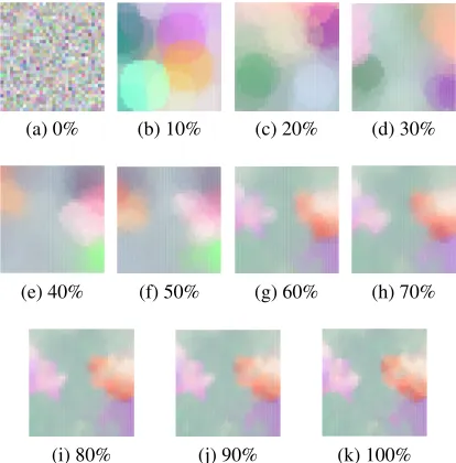
Figure 5: Development of SOM Top 10 categories vectorized with 33,120 dimensions, 32x32 grid and 100 iterations.
In these experiments, documents were vectorized into 19,092 dimensions. Each vector was com-prised by TF-IDF values for ngrams ranging from
1to7, with a cut-off frequency of 10. While
doc-uments both in training and test sets could have multiple labels, each label was treated individually when predicting and scoring, as a series of single-label classification problems.
[image:6.612.86.293.47.257.2]5.3 Visualization of SOM Development Figure 5 shows the development of a Self-Organizing Map with a grid size of 32x32 from the experiments on the Top 10 categories. Dur-ing the first iteration steps, the radius of the ini-tial neighborhood is clearly visible before the grid self-organizes into a map. Each node is repre-sented by a vector with the same dimensionality as the vectorized documents; these node vectors were reduced to four dimensions using Principal Component Analysis (PCA) (Jolliffe, 1986).
The four values were then used to encode a color in the Matplotlib library (Hunter, 2007), dis-playing each node as a color grading. The library accepts vectors of both three and four dimensions to create colors, so in order to retain more of the variance in the original node vectors, the vectors were reduced to four dimensions. Similarity in colors visualize similarity between vectors in the same area. Document labels verify that these areas represent texts belonging to the same categories.
Figure 6: Annotated SOM with grid size 8x8 of the Top 10 categories, with highlighted excerpts. Training samples yellow, test samples magenta.
(a) top-left (purple) (b) bottom-left (green)
(c) middle (blue)
Figure 7: Excerpts from Figure 6 showing how document categories cluster.
5.4 Visualization of Resulting SOMs
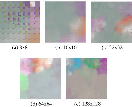
[image:6.612.329.516.330.631.2](a) 8x8 (b) 16x16 (c) 32x32
[image:7.612.83.301.46.222.2](d) 64x64 (e) 128x128
Figure 8: Various size SOMs, Top 10 categories.
low) and the test (magenta) samples.
The 8x8 map is used for illustration here since it is easier to show the contents of grid cells in this format. As the number of nodes grows larger, it is difficult to fit the areas in one frame.
Three excerpts of the 8x8 SOM of Figure 6 are detailed in Figure 7. Starting with Figure 7a, the cell in the top left corner of the map has three training corpus labels attaching to it,acq(41 doc-uments), earn (3) andinterest (1); and 14 docu-ments from the test corpus, all with the category acq. Majority voting among the training samples assigns the categoryacqto the node and hence en-sures that all of the test samples are labeled cor-rectly.
In Figure 7b, all documents — both from the training and test corpora — have the labelearn, so classification is straight-forward (and correct).
Finally, the four nodes in Figure 7c have at-tracted documents with multiple labels. The fig-ure shows four cells, each representing a node in the SOM. The yellow training labels are sorted in decreasing order from the left bottom up, and the magenta test labels in decreasing order from the left top corner of the cell.
The labels with the highest frequency both in the training and test corpora match all four cells in Figure 7c (interest,coffee,money-fxandcrude). Thus, these labels from the training corpus are the predictions for each node, and the set of correctly predicted test samples, respectively.
In addition to the most frequent labels, the lists in Figure 7c share many other members, indicating that the clustered documents have more properties in common.
(a) 8x8 (b) 16x16 (c) 32x32
[image:7.612.317.537.46.223.2](d) 64x64 (e) 128x128
Figure 9: Various size SOMs, all categories.
The final maps for the Top 10 category and all category runs are shown in Figures 8 and 9. In the larger maps there are fewer categories attaching to each node, both from training and test corpus. As can be seen from the results in Tables 2 and 3, macroaveraged F-scores increase as the grid sizes increase. With fewer categories per node, smaller categories have a better chance of being the major-ity category of a node, enabling the SOM to pre-dict that node.
Figure 8d shows a SOM with grid size 64x64. On the left side of the picture, a light green area is visible. The green area is populated by doc-uments labeled crude, going into an area labeled earnas the area turns gray in the vertical direction. Likewise, in the middle of the figure, areas pop-ulated by interest neighbor areas labeled money-supply. The map images are too large to include, and hence left out from the present paper.
Figure 10 complements the information of the color shadings. The heatmap shows the amount of documents attached to each node (having the node as their BMU). This number is not visible from the color gradings of the map Visualization, and offers insight into the relative size of these ar-eas. The Unified Distance Matrix (UDM) shows the differences between the nodes on the map. The UDM is computed by taking the average distance between each node and its immediate neighbors in 2D space. High distances between nodes are shown as peaks in Figure 10b, and low areas rep-resent clusters of similar vectors. Comparing Fig-ures 8d and 10a, the flat area on the UDM reflects the large area in the bottom right corner in the same gray shading.
(a) Heatmap
[image:8.612.103.270.44.357.2](b) Unified Distance Matrix
Figure 10: Heatmap and Unified Distance Matrix of SOM with grid size 64x64. Top 10 categories.
6 Discussion and Related Work
Using the unsupervised Self-Organizing Map ap-proach we observe relations between categories, both through clusters of documents belonging to similar categories being placed next to each other on the map, and also in terms of some nodes in the SOM attracting separate documents with themati-cally adjacent labels as their Best-Matching Unit, such asmoney-fxandinterest. This could be a re-flection of these documents being in a thematical intersection between topics, or outright belonging to both.
Wermter and Hung (2002) integrated the SOM with WordNet-based (Miller, 1995) semantic net-works for doing classification on the Reuters Cor-pus. Documents were represented bysignificance vectors, i. e., the degree to which the documents belong to certain preassigned topics, that were in turn calculated from the importance of words in each category.
Saarikoski (2009) performed several experi-ments on using Self-Organizing Maps for
In-formation Retrieval and document classification (Saarikoski et al., 2011), comparing the algorithm to other machine learning techniques. While they explained how the SOM was applied to the prob-lem, some factors that affect classification perfor-mance were unaccounted for, such as the param-eters for the SOM creation, notable grid size and learning rate. Restricting the classification to the Top 10 categories (by frequency) their best exper-iments had micro- and macroaverages of 93.2% and 83.5%, respectively.
Interestingly, Saarikoski et al. (2011) report that a Na¨ıve Bayes classifier outscored all other meth-ods on the data (95.2% and 90.4%), results that also significantly beat the findings of Dumais et al. (1998), who reported only 81.5% accuracy for the Na¨ıve Bayes method. This discrepancy is likely due to a difference in scoring, as Dumais et al. (1998) reported break-even scores (motivated by comparability with other research), as opposed to Saarikoski et al. (2011) that gave true accuracy scores without any adjustment for precision-recall trade-off. The break-even point is where the pre-cision is equal to recall, the point at which false positive and negative mis-classifications are done at the same rate.
Saarikoski et al. (2011) noticed how the costly training of SOMs is followed by cheap testing of new instances when doing classification, and sug-gested using multiple maps for multi-label clas-sification, or alternatively using the three near-est labels for a new instance. This would, how-ever, assume that all documents should have the same amount of labels in multi-label classification, which clearly is not the case in general. Still, it is possible to equip each node with a notion of label distribution, among its BMU training sam-ples, possibly within a region (neighborhood) of the BMU.
While we did not see an increase in the one-of classification when the Self-Organizing Map topologies went above 32x32 nodes, it is likely that the multi-label problem benefits from a larger amount of nodes, offering finer granularity.
7 Conclusion and Future Work
SOM affects classification performance. We ob-serve that classification performance increases up to the size of 32x32 nodes, and then deteriorates for the vectorizations used in the experiments. The paper offers extensive details on the parameters used to create the SOMs.
Using the Self-Organizing Map analysis, we observe underlying relations between documents, visible in 2D space, although represented with high-dimensional vectors. In the Self-Organizing Maps, similarities betweenlabelsas well as simi-larities between individual documents are visible. We therefore argue that the simplification of the multi-labelclassification task to a cascade of bi-nary classification tasks is not plausible for the Reuters Corpus, because of the presence of rela-tions between labels.
Further research into the multi-label problem and its relation to large-topology Self-Organizing Maps is prudent, given the findings of the present work. Devising a fair evaluation scheme for mea-suring the accuracy of SOM classifiers that at-tribute many labels to each document instance as a multi-label problem, is still an open question. Similarly, it is also an open question which method to use to decide how many labels to attribute to a new training instance. It is a natural next step to run more experiments on attributing several labels to documents in one operation and comparing that to running a series of binary classifications, as in the experiments presented in this paper.
Having implemented the Self-Organizing Map algorithm in a highly modular fashion, we would also like to experiment with both a) using differ-ent vectorizers and b) applying differdiffer-ent distances metrics, in order to investigate their impact on classification results. Wermter and Hung (2002) reported good results on integrating other knowl-edge sources in vectorization, calling for a system-atic comparison to purely data-driven vector trans-formers, and to hybrids between knowledge- and data-driven vectorizers.
Acknowledgments
The research leading to these results has been funded by Norwegian University of Science and Technology (NTNU), and by the Norwegian Re-search Council (NFR) and the Czech Ministry of Education, Youth and Sports (MˇSMT) through the Norwegian Financial Mechanism 2009–2014 un-der Contract no. MSMT-28477/2014.
References
Lars Asker, Atelach Alemu Argaw, Bj¨orn Gamb¨ack, Samuel Eyassu Asfeha, and Lemma Nigussie Habte. 2009. Classifying Amharic webnews. Information Retrieval, 12(3):416–435.
Junli Chen, Xuezhong Zhou, and Zhaohui Wu. 2004. A multi-label Chinese text categorization system based on boosting algorithm. InProceedings of the Fourth International Conference on Computer and Information Technology, pages 1153–1158, Wash-ington, DC, USA. IEEE Computer Society.
Franca Debole and Fabrizio Sebastiani. 2004. An anal-ysis of the relative hardness of Reuters-21578 sub-sets. Journal of the American Society for Informa-tion Science and Technology, 56:971–974.
Scott Deerwester, Susan T. Dumais, George W. Fur-nas, Thomas K. Landauer, and Richard Harshman. 1990. Indexing by latent semantic analysis. Jour-nal of the American Society for Information Science, 41(6):391–407.
Susan Dumais, John Platt, Mehran Sahami, and David Heckerman. 1998. Inductive learning algorithms and representations for text categorization. In Pro-ceedings of the 7th International Conference on In-formation and Knowledge Management, pages 148– 155. ACM Press.
Samuel Eyassu and Bj¨orn Gamb¨ack. 2005. Classify-ing Amharic news text usClassify-ing Self-OrganizClassify-ing Maps. In Proceedings of the 43rd Annual Meeting of the Association for Computational Linguistics, Ann Ar-bor, Michigan, June. ACL. Workshop on Computa-tional Approaches to Semitic Languages.
Jean-Claude Fort, Patrick Letr´emy, and Marie Cottrell. 2002. Advantages and drawbacks of the Batch Ko-honen algorithm. In Michel Verleysen, editor, Pro-ceedings of the 10th European Symposium on Artifi-cial Neural Networks, pages 223–230, Bruges, Bel-gium.
John D. Hunter. 2007. Matplotlib: A 2D graphics en-vironment. Computing in Science & Engineering, 9(3):90–95.
Heikki Hy¨otyniemi. 1996. Text document classifi-cation with self-organizing maps. In J. Alander, T. Honkela, and M. Jakobsson, editors, Proceed-ings of 7th Finnish Artificial Intelligence Confer-ence, pages 64–72, Vaasa, Finland.
Ian T. Jolliffe. 1986. Principal Component Analysis. Springer Verlag, New York, NY, USA.
Teuvo Kohonen, Samuel Kaski, Krista Lagus, and Timo Honkela. 1996. Very large two-level SOM for the browsing of newsgroups. In C. von der Malsburg, W. von Seelen, J. C. Vorbr¨uggen, and B. Sendhoff, editors,Proceedings of ICANN96, In-ternational Conference on Artificial Neural Net-works, Lecture Notes in Computer Science, vol. 1112, pages 269–274. Springer, Berlin, July.
Teuvo Kohonen. 1982. Self-organized formation of topologically correct feature maps. Biological Cy-bernetics, 43(1):59–69.
Richard D. Lawrence, George S. Almasi, and Holly E. Rushmeier. 1999. A scalable parallel algorithm for self-organizing maps with applications to sparse data mining problems. Data Mining and Knowledge Discovery, 3(2):171–195.
David D. Lewis, Yiming Yang, Tony G. Rose, and Fan Li. 2004. RCV1: A new benchmark collection for text categorization research.Journal of Machine Learning Research, 5:361–397, December.
David D. Lewis. 1997. Reuters-21578 text categoriza-tion test colleccategoriza-tion.
http://www.daviddlewis.com/ resources/testcollections/
reuters21578/.
Zhen-Ping Lo, Masahiro Fujita, and Behnam Bavarian. 1991. Analysis of neighborhood interaction in Ko-honen neural networks. InProceedings of the Fifth International Parallel Processing Symposium, pages 246–249. IEEE.
Edward Loper and Steven Bird. 2002. NLTK: The nat-ural language toolkit. InProceedings of the ACL-02 Workshop on Effective Tools and Methodologies for Teaching Natural Language Processing and Com-putational Linguistics - Volume 1, ETMTNLP ’02, pages 63–70, Stroudsburg, PA, USA. Association for Computational Linguistics.
Christopher D. Manning, Prabhakar Raghavan, and Hinrich Sch¨utze. 2008. Introduction to Information Retrieval. Cambridge University Press, New York, NY, USA.
George A. Miller. 1995. WordNet: A lexical database for English. Communications of the ACM, 38(11):39–41, November.
Bhavik Patel, Anurag Jajoo, Yash Tibrewal, and Amit Joshi. 2015. An efficient parallel algorithm for self-organizing maps using MPI-OpenMP based cluster. International Journal of Computer Applications, IJCA Proceedings on International Conference on Advanced Computing and Communication Tech-niques for High Performance Applications(2):5–9, February.
Fabian Pedregosa, Ga¨el Varoquaux, Alexandre Gram-fort, Vincent Michel, Bertrand Thirion, Olivier Grisel, Mathieu Blondel, Peter Prettenhofer, Ron Weiss, Vincent Dubourg, Jake Vanderplas, Alexan-dre Passos, David Cournapeau, Matthieu Brucher, Matthieu Perrot, and ´Edouard Duchesnay. 2011. Scikit-learn: Machine learning in Python. Journal of Machine Learning Research, 12(1):2825–2830.
Jyri Saarikoski, Jorma Laurikkala, Kalervo J¨arvelin, and Martti Juhola. 2011. Self-organising maps in document classification: A comparison with six ma-chine learning methods. In Andrej Dobnikar, Uroˇs Lotric, and Branko ˇSter, editors,Adaptive and Natu-ral Computing Algorithms: 10th International Con-ference, ICANNGA 2011, Ljubljana, Slovenia, April 14-16, 2011, Proceedings, Part I, volume 6593 of Lecture Notes in Computer Science, pages 260–269. Springer.
Jyri Saarikoski. 2009. A study on the use of self-organised maps in information retrieval. Journal of Documentation, 65(2):304–322.
Fabrizio Sebastiani. 2002. Machine learning in au-tomated text categorization. ACM Computing Sur-veys, 34(1):1–47, March.
Stefan Wermter and Chihli Hung. 2002. Self-organizing classification on the Reuters news cor-pus. InProceedings of the 19th International Con-ference on Computational Linguistics - Volume 1, COLING ’02, pages 1–7, Stroudsburg, PA, USA. Association for Computational Linguistics.
Yiming Yang and Xin Liu. 1999. A re-examination of text categorization methods. In Proceedings of the 22nd Annual International ACM SIGIR Confer-ence on Research and Development in Information Retrieval, SIGIR ’99, pages 42–49, New York, NY, USA. ACM.
Shuang-Hong Yang, Hongyuan Zha, and Bao-Gang Hu. 2009. Dirichlet-Bernoulli alignment: A genera-tive model for multi-class multi-label multi-instance corpora. In Y. Bengio, D. Schuurmans, J.D. Laf-ferty, C.K.I. Williams, and A. Culotta, editors, Ad-vances in Neural Information Processing Systems 22, pages 2143–2150. Curran Associates, Inc.