Robust Logistic Regression using Shift Parameters

Robust Logistic Regression using Shift Parameters

Julie TibshiraniandChristopher D. Manning Stanford University

Stanford, CA 94305, USA

{jtibs, manning}@cs.stanford.edu

Abstract

Annotation errors can significantly hurt classifier performance, yet datasets are only growing noisier with the increased use of Amazon Mechanical Turk and tech-niques like distant supervision that auto-matically generate labels. In this paper, we present a robust extension of logistic regression that incorporates the possibil-ity of mislabelling directly into the objec-tive. This model can be trained through nearly the same means as logistic regres-sion, and retains its efficiency on high-dimensional datasets. We conduct exper-iments on named entity recognition data and find that our approach can provide a significant improvement over the standard model when annotation errors are present.

1 Introduction

Almost any large dataset has annotation errors, especially those complex, nuanced datasets com-monly used in natural language processing. Low-quality annotations have become even more com-mon in recent years with the rise of Amazon Me-chanical Turk, as well as methods like distant su-pervision and co-training that involve automati-cally generating training data.

Although small amounts of noise may not be detrimental, in some applications the level can be high: upon manually inspecting a relation ex-traction corpus commonly used in distant super-vision, Riedel et al. (2010) report a 31% false positive rate. In cases like these, annotation er-rors have frequently been observed to hurt perfor-mance. Dingare et al. (2005), for example, con-duct error analysis on a system to extract relations from biomedical text, and observe that over half of the system’s errors could be attributed to incon-sistencies in how the data was annotated. Simi-larly, in a case study on co-training for natural

lan-guage tasks, Pierce and Cardie (2001) find that the degradation in data quality from automatic la-belling prevents these systems from performing comparably to their fully-supervised counterparts. In this work we argue that incorrect exam-ples should be explicitly modelled during train-ing, and present a simple extension of logistic re-gression that incorporates the possibility of mis-labelling directly into the objective. Following a technique from robust statistics, our model intro-duces sparse ‘shift parameters’ to allow datapoints to slide along the sigmoid, changing class if ap-propriate. It has a convex objective, is well-suited to high-dimensional data, and can be efficiently trained with minimal changes to the logistic re-gression pipeline.

In experiments on a large, noisy NER dataset, we find that this method can provide an improve-ment over standard logistic regression when anno-tation errors are present. The model also provides a means to identify which examples were misla-belled: through experiments on biological data, we demonstrate how our method can be used to accurately identify annotation errors. This robust extension of logistic regression shows particular promise for NLP applications: it helps account for incorrect labels, while remaining efficient on large, high-dimensional datasets.

2 Related Work

Much of the previous work on dealing with anno-tation errors centers around filtering the data be-fore training. Brodley and Friedl (1999) introduce what is perhaps the simplest form of supervised filtering: they train various classifiers, then record their predictions on a different part of the train set and eliminate contentious examples. Sculley and Cormack (2008) apply this approach to spam fil-tering with noisy user feedback.

One obvious issue with these methods is that the noise-detecting classifiers are themselves trained

on noisy labels. Unsupervised filtering tries to avoid this problem by clustering training instances based solely on their features, then using the clus-ters to detect labelling anomalies (Rebbapragada et al., 2009). Recently, Intxaurrondo et al. (2013) applied this approach to distantly-supervised rela-tion extracrela-tion, using heuristics such as the num-ber of mentions per tuple to eliminate suspicious examples.

Unsupervised filtering, however, relies on the perhaps unwarranted assumption that examples with the same label lie close together in feature space. Moreover filtering techniques in general may not be well-justified: if a training example does not fit closely with the current model, it is not necessarily mislabelled. It may represent an important exception that would improve the over-all fit, or appear unusual simply because we have made poor modelling assumptions.

Perhaps the most promising approaches are those that directly model annotation errors, han-dling mislabelled examples as they train. This way, there is an active trade-off between fitting the model and identifying suspected errors. Bootkra-jang and Kaban (2012) present an extension of logistic regression that models annotation errors through flipping probabilities. While intuitive, this approach has shortcomings of its own: the objec-tive function is nonconvex and the authors note that local optima are an issue, and the model can be difficult to fit when there are many more fea-tures than training examples.

There is a growing body of literature on learn-ing from several annotators, each of whom may be inaccurate (Bachrach et al., 2012; Raykar et al., 2009). It is important to note that we are consid-ering a separate, and perhaps more general, prob-lem: we have only one source of noisy labels, and the errors need not come from the human annota-tors, but could be introduced through contamina-tion or automatic labelling.

The field of ‘robust statistics’ seeks to develop estimators that are not unduly affected by devi-ations from the model assumptions (Huber and Ronchetti, 2009). Since mislabelled points are one type of outlier, this goal is naturally related to our interest in dealing with noisy data, and it seems many of the existing techniques would be relevant. A common strategy is to use a modi-fied loss function that gives less influence to points far from the boundary, and several models along

-4 -2 0 2 4

0.0

0.2

0.4

0.6

0.8

1.0

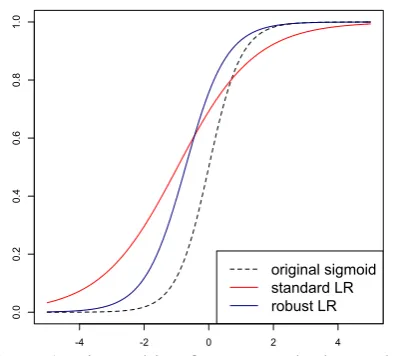
original sigmoid standard LR robust LR

Figure 1: Fit resulting from a standard vs. robust model, where data is generated from the dashed sigmoid and negative labels flipped with probabil-ity 0.2.

these lines have been proposed (Ding and Vish-wanathan., 2010; Masnadi-Shirazi et al., 2010). Unfortunately these approaches require optimiz-ing nonstandard, often nonconvex objectives, and fail to give insight into which datapoints are mis-labelled.

In a recent advance, She and Owen (2011) demonstrate that introducing a regularized ‘shift parameter’ per datapoint can help increase the ro-bustness of linear regression. Candes et al. (2009) propose a similar approach for principal compo-nent analysis, while Wright and Ma (2009) ex-plore its effectiveness in sparse signal recovery. In this work we adapt the technique to logistic re-gression. To the best of our knowledge, we are the first to experiment with adding ‘shift param-eters’ to logistic regression and demonstrate that the model is especially well-suited to the type of high-dimensional, noisy datasets commonly used in NLP.

3 Model

Recall that in binary logistic regression, the prob-ability of an examplexibeing positive is modeled as

g(θT_x

i) = _{1 +e}1_−θT_xi.

For simplicity, we assume the intercept term has been folded into the weight vectorθ, soθ∈Rm+1

wheremis the number of features.

pa-rameterγiso that the sigmoid becomes

g(θT_x

i+γi) = _{1 +e−}1_θT_xi−γi.

Since we believe that most examples are correctly labelled, weL1-regularize the shift parameters to

encourage sparsity. Lettingyi ∈ {0,1}be the la-bel for datapointiand fixingλ≥0, our objective is now given by

l(θ, γ) =Xn

i=1 h

yilogg(θTxi+γi) (1)

+ (1−yi) log 1−g(θTxi+γi)i−λ n X

i=1

|γi|.

These parametersγi let certain datapoints shift along the sigmoid, perhaps switching from one class to the other. If a datapointiis correctly an-notated, then we would expect its corresponding γi to be zero. If it actually belongs to the posi-tive class but is labelled negaposi-tive, thenγimight be positive, and analogously for the other direction.

One way to interpret the model is that it al-lows the log-odds of select datapoints to be shifted. Compared to models based on label-flipping, where there is a global set of flipping probabilities, our method has the advantage of tar-geting each example individually.

It is worth noting that there is no difficulty in regularizing theθ parameters as well. For exam-ple, if we choose to use an L1 penalty then our

objective becomes

l(θ, γ) = n X

i=1 h

yilogg(θTxi+γi) (2)

+ (1−yi) log 1−g(θTxi+γi)i

−κ

m X

j=1

|θj| −λ

n X

i=1

|γi|.

Finally, it may seem concerning that we have introduced a new parameter for each datapoint. But in many applications the number of features already exceedsn, so with proper regularization, this increase is actually quite reasonable.

3.1 Training

Notice that adding these shift parameters is equiv-alent to introducingnfeatures, where theith new feature is1for datapointiand0otherwise. With

this observation, we can simply modify the fea-ture matrix and parameter vector and train the lo-gistic model as usual. Specifically, we let θ0 ₌

(θ0, . . . , θm, γ1, . . . , γn)andX0 = [X|In]so that

the objective (1) simplifies to

l(θ0) =

n X

i=1 h

yilogg(θ0Tx0_i)

+ (1−yi) log 1−g(θ0Tx0i) i

−λmX+n

j=m+1

|θ0(j)_|.

Upon writing the objective in this way, we imme-diately see that it is convex, just as standard L1

-penalized logistic regression is convex.

3.2 Testing

To obtain our final logistic model, we keep only the θ parameters. Predictions are then made as usual:

I{g(ˆθT_x)>0.5}.

3.3 Selecting Regularization Parameters

The parameter λ from equation (1) would nor-mally be chosen through cross-validation, but our set-up is unusual in that the training set may con-tain errors, and even if we have a designated devel-opment set it is unlikely to be error-free. We found in simulations that the errors largely do not inter-fere in selectingλ, so in the experiments below we cross-validate as normal.

Notice thatλhas a direct effect on the number of nonzero shiftsγ and hence the suspected num-ber of errors in the training set. So if we have in-formation about the noise level, we can directly incorporate it into the selection procedure. For ex-ample, we may believe the training set has no more than 15% noise, and so would restrict the choice ofλduring cross-validation to only those values where 15% or fewer of the estimated shift param-eters are nonzero.

We now consider situations in which theθ pa-rameters are regularized as well. Assume, for ex-ample, that we use L1-regularization as in

equa-tion (2), so that we now need to optimize over both κandλ. We perform the following simple proce-dure:

1. Cross-validate using standard logistic regres-sion to selectκ.

method suspects identified false positives

Alon et al. (1999) T2 T30 T33 T36 T37 N8 N12 N34 N36

Furey et al. (2000) • • • • • •

Kadota et al. (2003) • • • • • T6, N2

Malossini et al. (2006) • • • • • • • T8, N2, N28, N29

Bootkrajang et al. (2012) • • • • • • •

Robust LR • • • • • • •

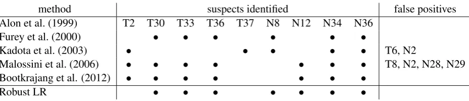
Table 1: Results of various error-identification methods on the colon cancer dataset. The first row lists the samples that are biologically confirmed to be suspicious, and each other row gives the output from an automatic detection method. Bootkrajang et al. report confidences, so we threshold at 0.5 to obtain these results.

4 Experiments

We conduct two sets of experiments to assess the effectiveness of the approach, in terms of both identifying mislabelled examples and producing accurate predictions.

4.1 Contaminated Data

Our first experiment is centered around a biologi-cal dataset with suspected labelling errors. Called the colon cancer dataset, it contains the expres-sion levels of 2000 genes from 40 tumor and 22 normal tissues (Alon et al., 1999). There is evi-dence in the literature that certain tissue samples may have been cross-contaminated. In particular, 5 tumor and 4 normal samples should have their labels flipped.

In this experiment, we examine the model’s ability to identify mislabelled training examples. Because there are many more features than data-points and it is likely that not all genes are relevant, we choose to place anL1penalty onθ.

Usingglmnet, an R package for training reg-ularized models (Friedman et al., 2009), we se-lect κ and λ using cross-validation. Looking at the resulting values for γ, we find that only 7 of the shift parameters are nonzero and that each one corresponds to a suspicious datapoint. As further confirmation, the signs of the gammas correctly match the direction of the mislabelling. Compared to previous attempts to automatically detect errors in this dataset, our approach identifies at least as many suspicious examples but with no false posi-tives. A detailed comparison is given in Table 1. Although Bootkrajang and Kaban (2012) are quite accurate, it is worth noting that due to its noncon-vexity, their model needed to be trained 20 times to achieve these results.

4.2 Manually Annotated Data

We now consider the problem of named entity

recognition(NER) to evaluate how our model

per-forms in a large-scale prediction task. In tradi-tional NER, the goal is to determine whether each word is a person, organization, location, or not a named entity (‘other’). Since our model is binary, we concentrate on the task of deciding whether a word is a person or not. (This task does not triv-ially reduce to finding the capitalized words, as the model must distinguish between people and other named entities like organizations).

For training, we use a large, noisy NER dataset collected by Jenny Finkel. The data was created by taking various Wikipedia articles and giving them to five Amazon Mechanical Turkers to anno-tate. Few to no quality controls were put in place, so that certain annotators produced very noisy la-bels. To construct the train set we chose a Turker who was about average in how much he disagreed with the majority vote, and used only his annota-tions. Negative examples are subsampled to bring the class ratio to a reasonable level, for a total of 200,000 negative and 24,002 positive examples. We find that in 0.4% of examples, the majority agreed they were negative but the chosen annota-tor marked them positive, and 7.5% were labelled positive by the majority but negative by the an-notator. Note that we still include examples for which there was no majority consensus, so these noise estimates are quite conservative.

We evaluate on the English development test set from the CoNLL shared task (Tjong Kim Sang and Meulder, 2003). This data consists of news arti-cles from the Reuters corpus, hand-annotated by researchers at the University of Antwerp.

model precision recall F1

standard 76.99 85.87 81.19

flipping 76.62 86.28 81.17

robust 77.04 90.47 83.22

Table 2: Performance of standard vs. robust logis-tic regression in the Wikipedia NER experiment. The flipping model refers to the approach from Bootkrajang and Kaban (2012).

chosen for simplicity and is not highly engineered – it largely consists of lexical features such as the current word, the previous and next words in the sentence, as well as character n-grams and vari-ous word shape features. With a total of 393,633 features in the train set, we choose to use L2

-regularization, so that our penalty now becomes

1 2σ2

m X

j=0

|θj|2+λXn

i=1

|γi|.

This choice is natural asL2 is the most common

form of regularization in NLP, and we wish to ver-ify that our approach works for penalties besides

L1.

The robust model is fit using Orthant-Wise Limited-Memory Quasi Newton (OWL-QN), a technique for optimizing an L1-penalized

objec-tive (Andrew and Gao, 2007). We tune both models through 5-fold cross-validation to obtain σ2 _{= 1.0andλ = 0.1. Note that from the way}

we cross-validate (first tuningσusing standard lo-gistic regression, fixing this choice, then tuningλ) our procedure may give an unfair advantage to the baseline.

We also compare against the algorithm pro-posed in Bootkrajang and Kaban (2012), an exten-sion of logistic regresexten-sion mentioned in the section on prior work. This approach assumes that each example’s true label is flipped with a certain prob-ability before being observed, and fits the resulting latent-variable model using EM.

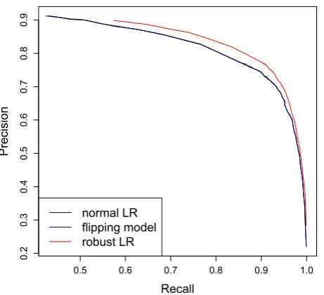
The results of these experiments are shown in Table 2 as well as Figure 2. Robust logistic re-gression offers a noticeable improvement over the baseline, and this improvement holds at essentially all levels of precision and recall. Interestingly, be-cause of the large dimension, the flipping model consistently learns that no labels have been flipped and thus does not show a substantial difference with standard logistic regression.

0.5 0.6 0.7 0.8 0.9 1.0

0.2

0.3

0.4

0.5

0.6

0.7

0.8

0.9

Recall

Pre

ci

si

on

normal LR flipping model

robust LR

Figure 2: Precision-recall curve obtained from training on noisy Wikipedia data and testing on CoNLL. The flipping model refers to the approach from Bootkrajang and Kaban (2012).

5 Future Work

A natural direction for future work is to extend the model to a multi-class setting. One option is to introduce aγ for every class except the negative one, so that there aren(c−1)shift parameters in all. We could then apply a group lasso, with each group consisting of theγfor a particular datapoint (Meier et al., 2008). This way all of a datapoint’s shift parameters drop out together, which corre-sponds to the example being correctly labelled.

CRFs and other sequence models could also benefit from the addition of shift parameters. Since the extra variables can be neatly folded into the linear term, convexity is preserved and the model could essentially be trained as usual.

Acknowledgments

References

U. Alon, N. Barkai, D. A. Notterman, K. Gish, S. Ybarra, D. Mack, A. J. Levine. 1999. Broad patterns of gene expression revealed by clustering analysis of tumor and normal colon tissues probed by oligonucleotide arrays. National Academy of Sci-ences of the USA.

Galen Andrew and Jianfeng Gao. 2007.

Scal-able Training of L1-Regularized Log-Linear

Mod-els. ICML.

Yoram Bachrach, Thore Graepel, Tom Minka, and John Guiver. 2012. How To Grade a Test With-out Knowing the Answers: A Bayesian Graphical Model for Adaptive Crowdsourcing and Aptitude Testing.arXiv preprint arXiv:1206.6386 (2012).

Jakramate Bootkrajang and Ata Kaban. 2012. Label-noise Robust Logistic Regression and Its

Applica-tions. ECML PKDD.

Carla E. Brodley and Mark A. Friedl. 1999.

Identify-ing mislabeled TrainIdentify-ing Data. JAIR,11, 131-167.

Emmanuel J. Candes, Xiaodong Li, Yi Ma, John Wright. 2009. Robust Principal Component

Analy-sis? arXiv preprint arXiv:0912.3599, 2009.

Nan Ding and S. V. N. Vishwanathan. 2010. t-Logistic regression. NIPS.

Shipra Dingare, Malvina Nissim, Jenny Finkel, Christopher Manning, and Claire Grover. 2005. A system for identifying named entities in biomedical text: How results from two evaluations reflect on

both the system and the evaluations. Comparative

and Functional Genomics.6(1–2), 77-85.

Jenny Rose Finkel, Trond Grenager, Christopher Man-ning. 2005. Incorporating Non-local Information into Information Extraction Systems by Gibbs

Sam-pling. ACL.

Jerome Friedman, Trevor Hastie, Rob Tibshirani 2009. Regularization Paths for Generalized Linear Models via Coordinate Descent. Journal of statistical soft-ware,33(1), 1.

Terrence S. Furey, Nello Cristianini, Nigel Duffy, David W. Bednarski, Michel Schummer, David Haussler. 2000. Support vector machine classifi-cation and validation of cancer tissue samples using microarray expression data. Bioinformatics,16(10), 906-914.

Peter J. Huber and Elvezio M. Ronchetti. 2000.Robust Statistics.John Wiley & Sons, Inc., Hoboken, NJ. Ander Intxaurrondo, Mihai Surdeanu, Oier Lopez de

Lacalle, and Eneko Agirre. 2013. Removing

Noisy Mentions for Distant Supervision. Congreso

de la Sociedad Espaola para el Procesamiento del Lenguaje Natural.

Koji Kadota, Daisuke Tominaga, Yutaka Akiyama, Katsutoshi Takahashi. 2003. Detecting outlying samples in microarray data: A critical assessment of the effect of outliers on sample. ChemBio Infor-matics Journal,3(1), 30-45.

Andrea Malossini, Enrico Blanzieri, Raymond T. Ng. 2006. Detecting potential labeling errors in

microar-rays by data perturbation. Bioinformatics, 22(17),

2114-2121.

Hamed Masnadi-Shirazi, Vijay Mahadevan, and Nuno Vasconcelos. 2010. On the design of robust

classi-fiers for computer vision. IEEE International

Con-ference Computer Vision and Pattern Recognition. Lukas Meier, Sara van de Geer, Peter Buhlmann. 2008.

The group lasso for logistic regression. Journal of the Royal Statistical Society,70(1), 53-71.

David Pierce and Claire Cardie. 2001. Limitations of co-training for natural language learning from large

datasets. EMNLP.

Vikas Raykar, Shipeng Yu, Linda H. Zhao, Anna Jere-bko, Charles Florin, Gerardo Hermosillo Valadez, Luca Bogoni, and Linda Moy. 2009. Supervised learning from multiple experts: whom to trust when everyone lies a bit. ICML.

Umaa Rebbapragada, Lukas Mandrake, Kiri L. Wagstaff, Damhnait Gleeson, Rebecca Castano, Steve Chien, Carla E. Brodley 2009. Improv-ing Onboard Analysis of Hyperion Images by

Fil-tering mislabelled Training Data Examples. IEEE

Aerospace Conference.

Sebastian Riedel, Limin Yao, Andrew McCallum. 2010. Modeling Relations and Their Mentions

with-out Labelled Text.ECML PKDD.

D. Sculley and Gordon V. Cormack 2008. Filtering Email Spam in the Presence of Noisy User

Feed-back. CEAS.

Yiyuan She and Art Owen. 2011. Outlier Detection

Using Nonconvex Penalized Regression. Journal of

the American Statistical Association,106(494). Erik F. Tjong Kim Sang, Fien De Meulder. 2003.

Introduction to the CoNLL-2003 Shared Task: Language-Independent Named Entity Recognition. CoNLL.

John Wright and Yi Ma. 2009. Dense Error Correction vial1-Minimization IEEE Transactions on