A Syntax based Statistical Translation Model

(1)

A Syntax-based Statistical Translation Model

Kenji Yamada and Kevin Knight

Information Sciences Institute University of Southern California

4676 Admiralty Way, Suite 1001 Marina del Rey, CA 90292

kyamada,knight @isi.edu

Abstract

We present a syntax-based statistical translation model. Our model trans-forms a source-language parse tree into a target-language string by apply-ing stochastic operations at each node. These operations capture linguistic dif-ferences such as word order and case marking. Model parameters are esti-mated in polynomial time using an EM algorithm. The model produces word alignments that are better than those produced by IBM Model 5.

1 Introduction

A statistical translation model (TM) is a mathe-matical model in which the process of human-language translation is statistically modeled. Model parameters are automatically estimated us-ing a corpus of translation pairs. TMs have been used for statistical machine translation (Berger et al., 1996), word alignment of a translation cor-pus (Melamed, 2000), multilingual document re-trieval (Franz et al., 1999), automatic dictionary construction (Resnik and Melamed, 1997), and data preparation for word sense disambiguation programs (Brown et al., 1991). Developing a bet-ter TM is a fundamental issue for those applica-tions.

Researchers at IBM first described such a sta-tistical TM in (Brown et al., 1988). Their mod-els are based on a string-to-string noisy channel model. The channel converts a sequence of words in one language (such as English) into another (such as French). The channel operations are movements, duplications, and translations, ap-plied to each word independently. The movement

is conditioned only on word classes and positions in the string, and the duplication and translation are conditioned only on the word identity. Math-ematical details are fully described in (Brown et al., 1993).

One criticism of the IBM-style TM is that it does not model structural or syntactic aspects of the language. The TM was only demonstrated for a structurally similar language pair (English and French). It has been suspected that a language pair with very different word order such as En-glish and Japanese would not be modeled well by these TMs.

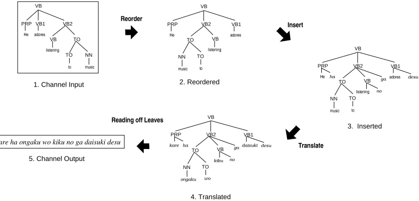
To incorporate structural aspects of the lan-guage, our channel model accepts a parse tree as an input, i.e., the input sentence is preprocessed by a syntactic parser. The channel performs ations on each node of the parse tree. The oper-ations are reordering child nodes, inserting extra words at each node, and translating leaf words. Figure 1 shows the overview of the operations of our model. Note that the output of our model is a string, not a parse tree. Therefore, parsing is only needed on the channel input side.

The reorder operation is intended to model translation between languages with different word orders, such as SVO-languages (English or Chi-nese) and SOV-languages (Japanese or Turkish). The word-insertion operation is intended to cap-ture linguistic differences in specifying syntactic cases. E.g., English and French use structural po-sition to specify case, while Japanese and Korean use case-marker particles.

(2)

1. Channel Input

3. Inserted

2. Reordered

kare ha ongaku wo kiku no ga daisuki desu

5. Channel Output

4. Translated

!

VB

PRP VB1 VB2

VB TO

TO NN

VB

VB2

TO

VB1

VB

PRP

!

NN

TO

VB

"#

$%&

# '()*

VB2

TO VB

VB1

PRP

!

NN

TO

VB

"#

$%&

# '()*

VB2

TO VB PRP

NN TO

VB1

+#,

(

%$

&

#+

*

+-+

*

'

# -)*

+

-.%

Figure 1: Channel Operations: Reorder, Insert, and Translate

nested structures.

Wu (1997) and Alshawi et al. (2000) showed statistical models based on syntactic structure. The way we handle syntactic parse trees is in-spired by their work, although their approach is not to model the translation process, but to formalize a model that generates two languages at the same time. Our channel operations are also similar to the mechanism in Twisted Pair Grammar (Jones and Havrilla, 1998) used in their knowledge-based system.

Following (Brown et al., 1993) and the other literature in TM, this paper only focuses the de-tails of TM. Applications of our TM, such as ma-chine translation or dictionary construction, will be described in a separate paper. Section 2 de-scribes our model in detail. Section 3 shows ex-perimental results. We conclude with Section 4, followed by an Appendix describing the training algorithm in more detail.

2 The Model

2.1 An Example

We first introduce our translation model with an example. Section 2.2 will describe the model more formally. We assume that an English parse tree is fed into a noisy channel and that it is trans-lated to a Japanese sentence.1

1

[image:2.595.93.511.72.273.2]

The parse tree is flattened to work well with the model. See Section 3.1 for details.

Figure 1 shows how the channel works. First, child nodes on each internal node are stochas-tically reordered. A node with / children has

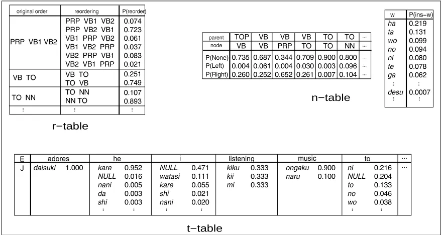
/10 possible reorderings. The probability of tak-ing a specific reordertak-ing is given by the model’s r-table. Sample model parameters are shown in Table 1. We assume that only the sequence of child node labels influences the reordering. In Figure 1, the top VB node has a child sequence

PRP-VB1-VB2. The probability of reordering it into PRP-VB2-VB1is 0.723 (the second row in the r-table in Table 1). We also reorder VB-TO

into TO-VB, andTO-NNinto NN-TO, so there-fore the probability of the second tree in Figure 1 is2436587:9<;=24365?>A@<;B243DC:@:9FEG243H>ACI> .

(3)

J KL M N J KJ J O J KP Q J

J KQR L J KJQ S J KPN P

J KM OO J KJ JO J KQ NP

J KLJ T J KJM J J KPQ S

J KT JJ J KJ JM J KJ JL

J KR J J J KJ T Q J KSJ O U V

W X Y U V U V

Y Z Y U V

W X U V

W X W X W[ X[

\]^_`ab \]cde fab \]ghi _b jklmno

npqm rrr

rrr rrr rrr rrr

s t

u

t

v w x w x y uz

{

t

|

z }~ J KP ST J KSM S J KJ T T J KJ T O J KJ R J J KJ L R J KJ Q P J KJ J JL

\]di

b

| t

y

} ~

y

S KJ J J

t

z

x

t

x y | t } s

y

J KT N P J KJ SQ J KJ J N J KJ J M J KJ J M

v

t

u

t

}

y

t z }s

y

x

t

x y

J KO L S J KSS S J KJ N N J KJ P S J KJ P J

yy y

y

~ J KMM M J KMM M J KMM M

w x{

t

~

x

t

~

J KT JJ J KSJJ

x y

u

w

x w v w

J KP SQ J KP J O J KSM M J KJ O Q J KJ M R

KKK KKK

Y Z Y U V S U VP Y Z Y U V P U V S U V S Y Z Y U VP U V S U V P Y Z Y U V P Y Z Y U V S U V P U V S Y Z Y

W X [ [ [ [

W X U V W X W X U V

J KJ L O J KL P M J KJ Q S J KJ M L J KJ R M J KJ P S

J KSJ L J KR T M J KP N S J KL O T Y Z Y U V

S

U V

P

W X [ [ U V W X

r−table

t−table

[image:3.595.78.518.72.306.2]

n−table

Table 1: Model Parameter Tables

parent=VB¡ node=PRP¢ is the conditioning in-dex. Using this label pair captures, for example, the regularity of inserting case-marker particles. When we decide which word to insert, no condi-tioning variable is used. That is, a function word like ga is just as likely to be inserted in one place as any other. In Figure 1, we inserted four words (ha, no, ga and desu) to create the third tree. The top VB node, two TO nodes, and the NN node inserted nothing. Therefore, the probability of obtaining the third tree given the second tree is

£

243D¤:¥:7¦;§243D74¨=@ª©«;

£

243D7:¥:7¦;§243¬2ª@I>©«;

£

243D7:¥:7¦;®243¬2ª¤:7ª©«;

£

243D7:¥:7F;B243¬2:2:2A5:©¯;B2436589:¥F;B24365I2ª@<;I243D@82:2°;I243DC82:2±E 3.498e-9.

Finally, we apply the translate operation to each leaf. We assume that this operation is depen-dent only on the word itself and that no context is consulted.2 The model’s t-table specifies the probability for all cases. Suppose we obtained the translations shown in the fourth tree of Figure 1. The probability of the translate operation here is

243D@:¥:7²;B243D@82:2°;=243¬2ª9:C<;=243D9:9:9<;A¨83¬2:2:2³EG243¬2´¨µ2ªC . The total probability of the reorder, insert and translate operations in this example is 243H>ACI>1; 3.498e-9 ;243¬2´¨µ2ªC1E 1.828e-11. Note that there

2

When a TM is used in machine translation, the TM’s role is to provide a list of possible translations, and a lan-guage model addresses the context. See (Berger et al., 1996).

are many other combinations of such operations that yield the same Japanese sentence. Therefore, the probability of the Japanese sentence given the English parse tree is the sum of all these probabil-ities.

We actually obtained the probability tables (Ta-ble 1) from a corpus of about two thousand pairs of English parse trees and Japanese sentences, completely automatically. Section 2.3 and Ap-pendix 4 describe the training algorithm.

2.2 Formal Description

This section formally describes our translation model. To make this paper comparable to (Brown et al., 1993), we use English-French notation in this section. We assume that an English parse tree ¶ is transformed into a French sentence · . Let the English parse tree ¶ consist of nodes ¸ª¹

¡

¸Bº 3µ3µ3=¡

¸B»

, and let the output French sentence consist of French words¼

¹

¡½¼

º

¡µ3µ3µ3?¡½¼I¾ .

(4)

to reorder them. This operation applies only to non-terminal nodes in the tree. Translation Á is an operation that translates a terminal English leaf word into a French word. This operation applies only to terminal nodes. Note that an English word can be translated into a French NULL word.

The notation ÄÅE ÇÆ

¡ÉÈÊ¡ÌËÍ¢ stands for a set of values of

¿Î¡ÌÀÏ¡½ÁÐ¢. ÄBÑ1E ÇÆ

ÑÒ¡ÉÈAÑÓ¡ÌËÔÑÇ¢ is a set of values of random variables associated with

¸

Ñ. And ÕÖE×Ä

¹

¡ÌÄ

º

¡µ3µ3µ3?¡ÌÄ

»

is the set of all ran-dom variables associated with a parse tree ¶ØE ¸:¹ ¡ ¸?º ¡µ3µ3µ3B¡ ¸=» .

The probability of getting a French sentence· given an English parse tree¶ is

PÙÛÚ=ÜÝÂÞàß á â4ã Strä â ä¬å§æçæçè:é PÙ â ÜÝ4Þ where Str £ Õ £

¶ê©É© is the sequence of leaf words of a tree transformed byÕ from¶ .

The probability of having a particular set of values of random variables in a parse tree is

PÙ

â

ÜÝÂÞëß PÙíìÔîÒïðì½ñ½ïÒòÓòÒòÉïóìÌôÜõµîÉïÇõ§ñ½ïÒòÓòÉòÒïÇõ½ôIÞ

ß ô ö÷ è î PÙíì ÷ ÜìÔîÉïóì½ñ§ïÒòÒòÒòÒïÇì ÷ ø îÉïùõ=îÓïÇõ§ñ§ïÒòÒòÒòÒïùõ§ô?Þúò

This is an exact equation. Then, we assume that a transform operation is independent from other transform operations, and the random variables of each node are determined only by the node itself. So, we obtain

PÙ

â

ÜÝÂÞàß PÙíì î ïóì ñ ïÒòÓòÒòÒïóì ô Üõ î ïÇõ ñ ïÒòÓòÒòÒïÇõ ô Þ

ß ô ö÷ è î PÙíì ÷ Üõ ÷ Þúò

The random variables Ä?Ñ<E ÇÆ

ÑÓ¡ÉÈÑú¡ÌËÔÑð¢ are as-sumed to be independent of each other. We also assume that they are dependent on particular fea-tures of the node¸

Ñ. Then,

PÙíì

÷

Üõ

÷

Þûß PÙíü

÷ ïùý ÷ ïÇþ ÷ Üõ ÷ Þ

ß PÙíü

÷

Üõ

÷

Þ PÙçý

÷

Üõ

÷

Þ PÙÛþ

÷

Üõ

÷

Þ

ß PÙíü

÷

Üÿ ÙÛõ

÷

ÞÇÞ PÙçý

÷

Ü

ÙÛõ

÷

ÞÇÞ PÙÛþ

÷

Ü ÙÛõ

÷

ÞÇÞ ß Ùíü

÷

Üÿ ÙÛõ

÷ ÞÇÞBÙçý ÷ Ü ÙÛõ ÷ ÞÇÞÒÙÛþ ÷

Ü ÙÛõ

÷

ÞÇÞ where , , and are the relevant features to

¿ ,À , andÁ , respectively. For example, we saw that the parent node label and the node label were used for , and the syntactic category sequence

of children was used for . The last line in the above formula introduces a change in notation, meaning that those probabilities are the model pa-rameters £ÇÆ © , £ È

©, and

£

Ë

©, where

, , and

are the possible values for , , and , respectively.

In summary, the probability of getting a French sentence· given an English parse tree¶ is

PÙÛÚ=ÜÝÂÞàß á â4ã Strä â ä¬å§æçæçè:é PÙ â ÜÝ4Þ ß á â4ã Strä â äHå®æçæèªé ô ö÷ è î Ùíü ÷ Üÿ ÙÛõ ÷ ÞÇÞBÙçý ÷ Ü ÙÛõ ÷ ÞÇÞÒÙÛþ ÷

Ü ÙÛõ

÷ ÞÇÞ where ÝØßëõ î ïÇõ ñ ïÒòÒòÒòÒïùõ ô and â ß ì î ïÇì ñ ïÒòÒòÉòÒïóì ô ß üBîÒïý:îÉïÇþ®îúï ü®ñ½ïÇý?ñ½ïÇþÉñúïÒòÒòÒòÉï ü®ô:ïùýBôªïùþÉô . The model parameters

£ÇÆ © ,

£

È

©, and

£

Ë

©, P

£ È © and P £ Ë

2.3 Automatic Parameter Estimation

To estimate the model parameters, we use the EM algorithm (Dempster et al., 1977). The algorithm iteratively updates the model parameters to max-imize the likelihood of the training corpus. First, the model parameters are initialized. We used a uniform distribution, but it can be a distribution taken from other models. For each iteration, the number of events are counted and weighted by the probabilities of the events. The probabilities of events are calculated from the current model pa-rameters. The model parameters are re-estimated based on the counts, and used for the next itera-tion. In our case, an event is a pair of a value of a random variable (such as

Æ

,È , orË ) and a feature value (such as

,

, or

). A separate counter is used for each event. Therefore, we need the same number of counters,

£ÇÆ ¡ ©, £ ÈÍ¡

©, and

£

Ë4¡

©, as the number of entries in the probability tables,

£ÇÆ © , £ È

£

Ë

© .

The training procedure is the following:

1. Initialize all probability tables: ÙíüÂÜ

Þ,?ÙçýAÜ

Þ, and ÓÙÛþ4Ü

Þ.

2. Reset all counters:§Ùíü?ï

Þ,§Ùçý:ï

Þ, and®ÙÛþ?ï

Þ.

3. For each pair

ÝÍïÚ in the training corpus,

For allâ

, such thatÚêß StrÙ

â

ÙíÝÂÞÇÞ,

Let cnt = PÙ

(5)

For!´ß#" òÒòÒò$ , ®Ùíü ïÛÿ ÙÛõ ÞÇÞ += cnt ®Ùçý

÷

ï

ÙÛõ

÷

ÞÇÞ += cnt ®ÙÛþ

÷

ï$ ÙÛõ

÷

ÞÇÞ += cnt

4. For each

üBï

,

ý:ï

, and

þ?ï

, ÍÙíüÜ

Þ ß%®Ùíü?ï

Þ '& ®Ùíü?ï

Þ

?ÙçýAÜ

Þ ß%®Ùçý:ï

Þ(*)+®Ùçý:ï

Þ

ÒÙÛþ4Ü

ÞÊß%®ÙÛþBï

Þ -, §ÙÛþ?ï

Þ

5. Repeat steps 2-4 for several iterations.

A straightforward implementation that tries all possible combinations of parameters

ÇÆ

¡ÉÈÍ¡ÌËÍ¢, is very expensive, since there are.

£/Æ

»

È

»

Æ and

È

are the num-ber of possible values for

Æ

andÈ , respectively (Ë is uniquely decided when

Æ

andÈ are given for a particular

¶¯¡Ì·I¢ ). Appendix describes an efficient implementation that estimates the probability in polynomial time.3 With this efficient implemen-tation, it took about 50 minutes per iteration on our corpus (about two thousand pairs of English parse trees and Japanese sentences. See the next section).

3 Experiment

To experiment, we trained our model on a small English-Japanese corpus. To evaluate perfor-mance, we examined alignments produced by the learned model. For comparison, we also trained IBM Model 5 on the same corpus.

3.1 Training

We extracted 2121 translation sentence pairs from a Japanese-English dictionary. These sentences were mostly short ones. The average sentence length was 6.9 for English and 9.7 for Japanese. However, many rare words were used, which made the task difficult. The vocabulary size was 3463 tokens for English, and 3983 tokens for Japanese, with 2029 tokens for English and 2507 tokens for Japanese occurring only once in the corpus.

Brill’s part-of-speech (POS) tagger (Brill, 1995) and Collins’ parser (Collins, 1999) were used to obtain parse trees for the English side of the corpus. The output of Collins’ parser was

3

Note that the algorithm performs full EM counting, whereas the IBM models only permit counting over a sub-set of possible alignments.

modified in the following way. First, to reduce the number of parameters in the model, each node was re-labelled with the POS of the node’s head word, and some POS labels were collapsed. For example, labels for different verb endings (such asVBDfor -ed andVBGfor -ing) were changed to the same labelVB. There were then 30 differ-ent node labels, and 474 unique child label se-quences.

Second, a subtree was flattened if the node’s word was the same as the parent’s head-word. For example, (NN1 (VB NN2))was flat-tened to (NN1 VB NN2) if the VB was a head word for bothNN1andNN2. This flattening was motivated by various word orders in different lan-guages. An English SVO structure is translated into SOV in Japanese, or into VSO in Arabic. These differences are easily modeled by the flat-tened subtree(NN1 VB NN2), rather than(NN1 (VB NN2)).

We ran 20 iterations of the EM algorithm as described in Section 2.2. IBM Model 5 was se-quentially bootstrapped with Model 1, an HMM Model, and Model 3 (Och and Ney, 2000). Each preceding model and the final Model 5 were trained with five iterations (total 20 iterations).

3.2 Evaluation

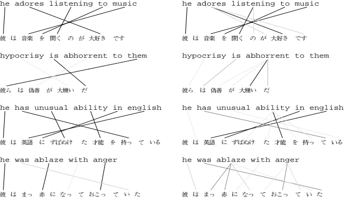
The training procedure resulted in the tables of es-timated model parameters. Table 1 in Section 2.1 shows part of those parameters obtained by the training above.

To evaluate performance, we let the models generate the most probable alignment of the train-ing corpus (called the Viterbi alignment). The alignment shows how the learned model induces the internal structure of the training data.

(6)

he adores listening to music

hypocrisy is abhorrent to them

he has unusual ability in english

he was ablaze with anger

he adores listening to music

hypocrisy is abhorrent to them

he has unusual ability in english

[image:6.595.129.467.68.263.2]

he was ablaze with anger

Figure 2: Viterbi Alignments: our model (left) and IBM Model 5 (right). Darker lines are judged more correct by humans.

The result was the following;

Alignment Perfect ave. score sents

Our Model 0.582 10

IBM Model 5 0.431 0

Our model got a better result compared to IBM Model 5. Note that there were no perfect align-ments from the IBM Model. Errors by the IBM Model were spread out over the whole set, while our errors were localized to some sentences. We expect that our model will therefore be easier to improve. Also, localized errors are good if the TM is used for corpus preparation or filtering.

We also measured training perplexity of the models. The perplexity of our model was 15.79, and that of IBM Model 5 was 9.84. For reference, the perplexity after 5 iterations of Model 1 was 24.01. Perplexity values roughly indicate the pre-dictive power of the model. Generally, lower per-plexity means a better model, but it might cause over-fitting to a training data. Since the IBM Model usually requires millions of training sen-tences, the lower perplexity value for the IBM Model is likely due to over-fitting.

4 Conclusion

We have presented a syntax-based translation model that statistically models the translation pro-cess from an English parse tree into a

foreign-language sentence. The model can make use of syntactic information and performs better for lan-guage pairs with different word orders and case marking schema. We conducted a small-scale ex-periment to compare the performance with IBM Model 5, and got better alignment results.

Appendix: An Efficient EM algorithm

This appendix describes an efficient implemen-tation of the EM algorithm for our translation model. This implementation uses a graph struc-ture for a pair

¶ ¡Ì·I¢ . A graph node is either a

major-node or a subnode. A major-node shows a pairing of a subtree of¶ and a substring of · . A subnode shows a selection of a value

ÇÆ

¡ÉÈÍ¡ÌËÍ¢ for the subtree-substring pair (Figure 3).

Let ·10

2

E ¼

2

3µ3µ3Ô¼ 234

065 ¹87

be a substring of · from the word¼

2

with length9. Note this notation is different from (Brown et al., 1993). A subtree

¸

Ñ is a subtree of¶ below the node

¸

Ñ. We assume that a subtree¸:¹

is¶ . A major-node :

£

¸

Ñ ¡Ì·;0

2

¸

Ñ and a substring · 0

2 . The root of the graph is

:

£

¸:¹ ¡Ì·1<

¹

©, where= is the length of· . Each major-node connects to several

Æ

-subnodes: £ÇÆ?>

¸

ÑÒ¡Ì· 0

2

©, showing which value of

Æ

is selected. The arc between :

£

¸

ÑÒ¡Ì·

0

2

¸

ÑÒ¡Ì·

0

2

£ÇÆ

¸

Ñð©. A

Æ

-subnode : £ÇÆ?>

¸

Ñ ¡Ì·10

2

final-node with weight P

£

Ë

¸

Ñó© if

¸

(7)

in ¶ . If

¸

Ñ is a non-terminal node, a -subnode connects to several È -subnodes :

£

È

>½Æ

¡

¸

ÑÉ¡Ì·;0

2

©, showing a selection of a value È . The weight of the arc is P

£

È

¸

Ñú©.

AÈ -subnode is then connected to @ -subnodes

:

£

@

>

ÈÊ¡

Æ

¡

¸

ÑÉ¡Ì·;0

2

©. The partition variable,@ , shows a particular way of partitioning· 0

2 . A@ -subnode:

£

@

>

ÈÍ¡

Æ

¡

¸

ÑÉ¡Ì· 0

2

Ñ and the substring of·10

2 , decided by ÇÆ

¡ÉÈÍ¡/@ ¢. A major-node can be connected from different @ -subnodes. The arc weights between È -subnodes and major-nodes are always 1.0.

ν

P

ρ

P

π

ABCDEFGDHI FJKLGDHI FJKLGDHI

(ρ|ε) (ν|ε)

[image:7.595.104.260.254.396.2]

FJKLGDHI ABCDEFGDHI

Figure 3: Graph structure for efficient EM train-ing.

This graph structure makes it easy to obtain P

£

Õ

ÕMStr

4

Õ

4ON 7P7PQSR P

£

Õ

Æ

-subnodes, and È -subnodes, and

all the arcs from @ -subnodes, corresponds to a particularÕ , and the product of the weight on the trace corresponds to P

£

Õ

¶ê©. Note that a trace forms a tree, making branches at the@ -subnodes. We define an alpha probability and a beta prob-ability for each major-node, in analogy with the measures used in the inside-outside algorithm for probabilistic context free grammars (Baker, 1979).

The alpha probability (outside probability) is a path probability from the graph root to the node and the side branches of the node. The beta proba-bility (inside probaproba-bility) is a path probaproba-bility be-low the node.

Figure 4 shows formulae for alpha-beta probabilities. From these definitions,

ÕMStr

4

Õ

4ON 7P7TQSR P

Õ ¶ © EVU ¸ª¹

¡Ì· <

¹

£ÇÆ

¡

© ,

£

ÈÊ¡

©, and

£

Ë4¡

¶ ¡Ì·I¢ are also in the figure. Those formulae replace the step 3 (in Section 2.3) for each training pair, and these counts are used in the step 4.

The graph structure is generated by expanding the root node:

£

¸:¹ ¡Ì·;<

¹

©. The beta probability for each node is first calculated bottom-up, then the alpha probability for each node is calculated top-down. Once the alpha and beta probabilities for each node are obtained, the counts are calculated as above and used for updating the parameters.

The complexity of this training algorithm is

.

£

XW Æ6

È

6

@

º

).

Acknowledgments

This work was supported by DARPA-ITO grant N66001-00-1-9814.

References

H. Alshawi, S. Bangalore, and S. Douglas. 2000.

Learning dependency translation models as

collec-tions of finite state head transducers.

Computa-tional Linguistics, 26(1).

J. Baker. 1979. Trainable grammars for speech recog-nition. In Speech Communication Papers for the

97th Meeting of the Acoustical Sciety of America.

A. Berger, P. Brown, S. Della Pietra, V. Della Pietra, J. Gillett, J. Lafferty, R. Mercer, H. Printz, and L. Ures. 1996. Language Translation Apparatus

and Method Using Context-Based Translation Mod-els. U.S. Patent 5,510,981.

E. Brill. 1995. Transformation-based error-driven

learning and natural language processing: A case study in part of specch tagging. Computational

Lin-guistics, 21(4).

P. Brown, J. Cocke, S. Della Pietra, F. Jelinek, R. Mer-cer, and P. Roossin. 1988. A statistical approach to language translation. In COLING-88.

P. Brown, J. Cocke, S. Della Pietra, F. Jelinek, R. Mer-cer, and P. Roossin. 1991. Word-sense disambigua-tion using statistical methods. In ACL-91.

P. Brown, S. Della Pietra, V. Della Pietra, and R. Mer-cer. 1993. The mathematics of statistical machine translation: Parameter estimation. Computational

(8)

oqp w;

6O68l

oqp\$ac[T8f6p wcw8

p ¡r

w

¢p£¤¡r

w ¥

® p8¯ wT°

±

Z[Ta6[]\$ac[nfc²¤p

w

ey\ yc[Pfbh³/Oyc´dbx[ny

±

ZeµlZ¶\$ac[+e(([nxe\·f6[]_`\$ac[T8fly;b$h¸m/¹1Z`e^`²¤p

w

ey\(y[Pfb$h¸i\Obacbxx[ny

±

Zeµ6ZX\a6[+µ6Z`e^xac[n b$h;³Oy´d`bxx[nyºm¤\/\a6[Tf p

w

ey+\?_`\a6[Tf]i\Obabx[ºbhq³/Oyc´d`bxx[ny]py»xe__`ej¶£$Oyc´dbx[nynm¤\/8Oy´d`bxx[ny

w

}ºp ¡r

w

\/ ¢p£¤¡r

w

\a6[¢f6Z[k\$a6µ

±

[nejZfly;hacb¼\$ac[T8f p

w

f6bS$} YZ[+d/[Pfl\(_acbd`\$de^efgiey[P½`[n¶\y

® p w¾

® pr$¿ctcuTÀ

Á

w

Â ¢pÃ¸¡r¿

w

eh¸r¿ ey\kf6[Ta6 e`\$^ ÄÆÅ

p ¡r¿

w

ÄÈÇ p£¤¡r¿

w

Ä

²É¶Ê ® pr·Êtcu

À

¦

Á

¦

w

eh¸r¿ ey\ºbx f6[Ta6 e`\$^

±

Z[Ta6[¢r·Ê¢ey\ µlZe^?b$hr ¿m\$`¶u

À

¦

Á

¦

ey\(_acb_/[Ta_`\$af6ef6eb$¶bh1u

À

Á

}

YZ[]µPb´8f6yË$p xtOÌ

w

mË$p£t6Í

w

m`\/?Ë$pÃt6Î

w

hb$a[n\µ6Z¶_`\eaºÏÐ;tcu·Ñ\a6[m

Ë$p tOÌ

w¾

Á·Ò

À

ÓcÔ`ÕcÖiÓcÔ

Ì

oqpr$¿6tcuTÀ

Á

w

¢p ¡r$¿ w`

Ç

¢p£¤¡r$¿ w`

²

¥

Ê

® prÊtcuTÀ¦

Á

¦

wn°º×

® pr8stcuvs;w

Ë$p£/t6Í w¾

ÁnÒ

À

ÓcÔ`ÕlØÓÔ

Í

oqpr$¿ctcuTÀ

Á

w

¢p£¡r$¿

w

Å

¢p ¡r$¿

w

²

¥

Ê

® prÊ tcuTÀ¦

Á

¦

wn°º× ® pr8stcu

vs w

ËpÃ`tcÎ

w¾

Á·Ò

À

ÓcÔ`ÕTÙ1ÓcÔ

Î

oqpr$¿ctcuTÀ

Á

w

pÃ¸¡r$¿ wT° ×

® pr8stcu vs

w

±

Z[Ta6[(z]ÚÜÛ?ÚÝpÞßàz

w

m`| ÚÜáÚâÞm\$`¶ÞâeyqfcZ[k^[Tj$f6Z¶b$hum`ye`µP[k\$¶ã1`j$^eycZ

±

ba6?µT\X(\flµ6Z¶\(ä¢åæ¸æ~a6[T`µ6Z

±

b$al¤}

Figure 4: Formulae for alpha-beta probabilities, and the count derivation

M. Collins. 1999. Head-Driven Statistical Models for

Natural Language Parsing. Ph.D. thesis,

Univer-sity of Pennsylvania.

A. Dempster, N. Laird, and D. Rubin. 1977. Max-imum likelihood from incomplete data via the em algorithm. Royal Statistical Society Series B, 39.

M. Franz, J. McCarley, and R. Ward. 1999. Ad hoc, cross-language and spoken document information retrieval at IBM. In TREC-8.

D. Jones and R. Havrilla. 1998. Twisted pair gram-mar: Support for rapid development of machine translation for low density languages. In AMTA98.

I. Melamed. 2000. Models of translational equiv-alence among words. Computational Linguistics, 26(2).

F. Och and H. Ney. 2000. Improved statistical align-ment models. In ACL-2000.

F. Och, C. Tillmann, and H. Ney. 1999. Improved alignment models for statistical machine transla-tion. In EMNLP-99.

P. Resnik and I. Melamed. 1997. Semi-automatic ac-quisition of domain-specific translation lexicons. In

ANLP-97.

Y. Wang. 1998. Grammar Inference and Statistical

Machine Translation. Ph.D. thesis, Carnegie

Mel-lon University.

D. Wu. 1997. Stochastic inversion transduction

grammars and bilingual parsing of parallel corpora.