THE APPLICABILITY OF BATCH TESTS TO ASSESS
BIOMETHANATION POTENTIAL OF ORGANIC WASTE AND ASSESS
SCALE UP TO CONTINUOUS REACTOR SYSTEMS
A thesis submitted in partial fulfilment of
the requirements for the Degree of PhD in
Environmental Engineering in the
University of Canterbury
by Nastaein Qamaruz Zaman
University of Canterbury
CONTENTS
NO. TITLE Page
ABSTRACT i
DEDICATIONS iii
ACKNOWLEDGEMENTS iv
LIST OF TABLES v
LIST OF FIGURES vii
1.0 CHAPTER 1: INTRODUCTION
1.1 Sustainable management of waste through anaerobic digestion 1
1.2 An overview of the anaerobic digestion process 1
1.2.1 Hydrolysis 2
1.2.2 Acid formation 3
1.2.2.1 Acidogenesis 3
1.2.2.2 Acetogenesis 3
1.2.3 Methanogenesis 3
1.2.4 Process balance 5
1.2.5 Kinetics 6
1.3 Measuring anaerobic biodegradation 6
1.3.1 Analysis of substrate consumption or product formation 7
1.3.1.1 COD, TOC, DOC 7
1.3.1.2 Uniformly 14C labeled test substances 7
1.3.1.3 Coenzyme F420 8
1.3.2 Analysis based on microbiological methods 8
1.3.2.1 Cloning of 16S rDNA 9
1.3.2.2 Denaturant gradient gel electrophoresis (DGGE) 10
1.3.2.3 Fluorescence in situ hybridisation (FISH) 12
1.3.3 Gasometric measurement techniques 13
1.3.3.1 The reactor 13
a) volumetric methods 14
b)manometric methods 16
1.3.4 Summary of anaerobic biodegradability tests 18
1.4 Anaerobic Digestion Feedstock 18
1.4.1 Feedstock potential 18
1.4.1.1 Agricultural waste 19
1.4.1.2 Energy crops 20
1.4.1.3 Industrial waste and wastewater 21
1.4.1.4 Municipal organic waste 22
1.4.1.5 Co-digestion 22
1.4.2 Issues with the feedstock 23
1.5 Research Need 26
1.6 Research Objective 27
1.7 Thesis Layout 28
2.0 CHAPTER 2: LITERATURE REVIEW
2.1 Introduction 30
Part 1: Methane potential determination
2.2 Available test methods 31
2.2.1 Biochemical methane potential test 32
2.2.2 Unspecified batch test 33
2.2.3 Gas measurement methods for batch anaerobic tests 35
2.2.4 Challenge AER-200 Respirometer 36
2.2.5 Anaerobic biogasification potential (ABP) 37
2.2.6 Biogas activity monitoring (BAM) 37
2.2.7 Summary 38
2.3 Standardisation of methane potential determination 40
2.4 Factors affecting methane potential tests 43
2.4.1 Equipment 44
2.4.2 Alkalinity 44
2.4.3 Liquid-to-void volume ratio 46
2.4.4 Incubation period 47
2.4.5 Incubation temperature 49
2.4.7 Inoculum 52
2.4.7.1 Seed source 52
2.4.7.2 Seed volume 54
2.4.7.3 Seed pre-treatment 55
a) Phase separation 56
b) Pre-digestion 57
2.4.8 Nutrient solution 59
2.4.9 Sample pre-treatment 61
2.5 Reproducibility and repeatability 63
Part 2: Anaerobic biodegradation kinetics
2.6 Introduction 65
2.6.1 The rate limiting step approach 66
2.6.2 Rates specific to various anaerobic digestion steps 66
2.6.3 Overall anaerobic digestion process 67
2.7 The first order kinetics 68
2.7.1 Introduction 68
2.7.2 At steady-state condition (continuous system) 68
2.7.3 Batch system 70
2.7.4 Hydrolysis rate constant 72
2.7.5 Overview of the IWA AD model 73
2.8 First order parameters 75
2.8.1 Method of estimation 75
2.8.1.1 Linear regression 76
2.8.1.2 Non-linear regression 78
2.8.2 Displays of digester operation 79
2.9 Weakness of the first order kinetic model 80
2.10 Coupling batch and continuous data 82
2.11 Summary of literature review 83
3.0 CHAPTER 3: METHODOLOGY
3.1 Introduction 86
3.2 Feedstock 87
3.2.1 Food waste 87
3.2.3 Cabbage 91
3.2.4 Rice 91
3.2.5 Glucose, starch and cellulose 92
3.3 Seed 92
3.4 Trace element 93
3.5 Alkali addition 94
3.6 Reactors 95
3.6.1 Tube batch reactor 95
3.6.2 Bottle batch reactor 96
3.6.3 Continuous reactor 97
3.7 Analytical methods 100
3.7.1 Gas analysis 100
3.7.1.1 Gas composition 100
a) Gas analyzer 100
b) Gas chromatography 102
3.7.1.2 Gas volume 104
3.7.2 Influent/Effluent analysis 107
3.7.2.1 pH 107
3.7.2.2 SCOD 107
3.7.2.3 Ammonia 108
3.7.2.4 Alkalinity 108
3.7.2.5 Volatile fatty acids 108
3.7.2.6 Solids content 111
a) Total solids 111
b) Total volatile solids 112
3.7.2.7 Moisture content 112
3.8 Suggestions for improvement 113
4.0 CHAPTER 4: TUBE DESIGN AND DEVELOPMENT
4.1 Introduction 115
4.2 Methodology 115
4.2.1 Seed 116
4.2.1.1 Seed source 116
4.2.1.3 Feasibility of seed pre-digestion 117
4.2.2 Substrate 118
4.2.3 Reproducibility issue 118
4.2.4 Assessment of total anaerobic biodegradability 119
4.2.4.1 Theoretical methane potential 119
4.2.4.2 Mixing 120
4.2.4.3 Trace elements 121
4.2.4.4 Buffer 121
4.2.4.5 Reactor headspace 121
4.3 Results 122
4.3.1 Anaerobic respirometer development 122
4.3.1.1 Design and procedure 122
4.3.1.2 Establishing food waste loading 122
4.3.2 Seed quality 129
4.3.2.1 Seed source 129
4.3.2.2 Seed thickening 130
4.3.2.3 Seed pre-digestion 132
4.3.3 Substrate loading 135
4.3.3.1 Cellulose, starch and glucose 135
4.3.3.2 Rice 138
4.3.3.3 Comparison between various substrates 140
4.3.4 Reproducibility of test results 141
4.3.4.1 Substrate influence 142
4.3.4.2 Seed influence 143
4.3.5 Establishing tube operating conditions 145
4.3.5.1 Experimental time 146
4.3.5.2 Mixing 148
4.3.5.3 Nutrient supplementation 150
4.3.5.4 Reactor headspace 152
4.4 Discussion 153
4.4.1 Tube design 153
4.4.2 Seed quality 154
4.4.3 Substrate loading 158
4.4.5 Tube operating procedure 162
4.4.5.1 Mixing 162
4.4.5.2 Experimental time 163
4.4.5.3 Nutrients 164
4.4.6 Reproducibility of results 166
4.5 Conclusion 168
4.6 Further work 170
5.0 CHAPTER 5: START UP PROCEDURE AND OPERATION OF A
CONTINUOUS REACTOR
5.1 Introduction 172
5.2 Methodology 173
5.2.1 Reactors 173
5.2.2 Parameters 175
5.2.2.1 Biogas composition 175
5.2.2.2 Effluent analysis 176
5.2.3 Start-up procedure 176
5.3 Results 177
5.3.1 A stable reactor 177
5.3.1.1 Substrate effects 179
5.3.1.2 Starting up a healthy reactor 181
5.3.2 Thresholds of reactor stability 185
5.3.2.1 pH 186
5.3.2.2 Ammonia 186
5.3.2.3 SCOD 187
5.3.2.4 VFA 189
5.3.2.5 Alkalinity 192
5.3.3 Factors and solutions for process imbalance 194
5.3.3.1 Washout 194
5.3.3.2 Inhibition 196
5.3.3.3 Temperature drop 197
5.4 Discussion 199
5.4.1.1 Reactor performance 199
5.4.1.2 Start-up 199
5.4.2 Thresholds of reactor stability 194
5.4.2.1 pH 194
5.4.2.2 Alkalinity 195
5.4.2.3 Volatile fatty acids 196
5.4.2.4 SCOD 198
5.4.2.5 Ammonia 199
5.4.2.6 H2 200
5.4.2.7 Relationship between the various parameters 200
5.4.3 Recommendation of suitable indicators 201
5.4.4 Factors and solutions for process imbalance 203
5.5 Conclusion 205
6.0 CHAPTER 6: KINETICS OF REACTION
6.1 Introduction 214
6.2 Methodology 215
6.2.1 Feedstock and inoculum 215
6.2.2 Experimental procedure 215
6.2.2.1 Food waste 215
6.2.2.2 Rice 216
6.2.3 Analyses 216
6.2.4 Kinetics 217
6.3 Result 218
6.3.1 Kinetics of individual reactor systems 218
6.3.1.1Food waste digestion 218
a) Batch tubes 218
b) Batch bottles 227
c) Continuous reactor 233
a) Batch tubes 236
b) Batch bottles 237
6.4 Discussion 242
6.4.1 Comparison of kinetics between various systems 242
6.4.2 Biodegradation rate of batch test and continuous reactor 244
6.4.3 First order reliability 246
6.4.4 Reproducibility of test results 248
6.5 Conclusions 252
6.6 Suggestions 253
7.0 CHAPTER 7: SUMMARY AND CONCLUDING STATEMENTS
7.1 Overview 254
7.2 Improved batch testing 255
7.3 Improved bench-scale CSTRs 258
7.4 Comparing batch and continuous system kinetics parameters 259
7.5 Future work 261
8.0 REFERENCES 263
Appendix 4-a Determination of the theoretical methane potential (TMP)
of food waste 281
Appendix 5-a Start-up procedure 285
Appendix 6-a The determination of first order kinetic parameters for batch
Tests; Bo, k, t lag and SSR 287
Appendix 6-b The estimation of expected methane yield from the volatile solids
of food wastes in tubes 290
Appendix 6-c Methane potential of food waste in bottle with modifications 293
i
ABSTRACT
Many of the current methods of assessing anaerobic biodegradability of solid samples require
sample modification prior to testing. Steps like sample drying, grinding, drying and
re-grinding to 2mm or less make the test results difficult to apply to field conditions and could
lead to oxygen exposure, possibly distorting the results. Finally, because of a small sample
size of about 10-50g w/w, the test result may not be representative of the bulk material.
A new tool dubbed ‘tube’ has been developed, made of 10 cm PVC pipe measuring 43.5
cm long with 3600 ml capacity with caps at both ends. For easy sample introduction, one
endcap is fixed while the other is screw capped. A distinctive feature is the wide neck
opening of about 10 cm where solid samples can be introduced as is, without further sample
modification.
Research has proven the tube applicable across various types of solid organic waste and
conditions provided that a suitable organic loading rate is determined. The tube is best
operated using 5-7 days pre-digested digested sewage sludge as seed, with minimal mixing
and without the addition of nutrients or alkali solution. The test result can be obtained within
4-6 days to 20 days, signifying a 50-75% and 95% substrate degradation, respectively.
Irreproducibility seen in some experiments may not only be a function of the seed and the
substrate. The organic loading rate (OLR) at which the test is conducted is also influential
especially if test is conducted closer to its maximum OLR tolerance where anaerobic process
is more erratic.
The performance of a continuous reactor digesting on a similar substrate can be estimated
using this new tool. Food waste is established by the tubes to have an ultimate methane
potential (B0) of 0.45L CH4/g VS. The same substrate when digested in a continuous reactor
ii and continuous are identical at 0.12 to 0.28 d-1. First order kinetics is efficient at modelling the anaerobic degradation when the process is healthy but may be less reliable under an
unstable process.
This research recommends the use of kinetics in combination with the experimental data (e.g.
HRT, OLR, yield) when planning and designing an industrial plant to avoid overdesign and
iii
DEDICATIONS
Thank you God, for the opportunities that have brought me where I am today. For giving the
strength to keep on striving when I am in despair. And for meeting me with such tremendous
and inviduals who helped and supported me throughout my time here in New Zealand.
This thesis is especially dedicated to my loving husband, Rojali. Thank you ayah, for the love
and care you have poured me, Haikal and Arissa. For the support and endurance you have
shown, making this thesis much easier to be completed. Our journey here has only
strengthened my love for all of you.
I am immensely appreciative of the support and encouragement by my parents, family and in
laws in Malaysia, in meeting this challenge. Thank you and may God repay your kindness.
Also, to all my friends, we have shared good times and difficult memories, which will remain
iv
ACKNOWLEDGEMENTS
This research has become a certainty due to the assistance and support of many individuals
and organisations. Hence, it is significant that contributions made by these important people
throughout the course of the research be presented in this thesis.
First and foremost, I would like to express my greatest gratitude to my supervisor, Dr Mark
Milke. His guidance and sound knowledge has been critical to the achievements and success
of the research. Mark’s motivation, devotion and vision have been nothing short of
inspirational. I am also thankful to the Environmental Laboratory technicians, Mr David
McPherson and Mr Peter McGuigan for their support and opinions particularly during the
experimentation stage. I gratefully acknowledge the co-operation by other postgraduates, Mr
Sudan Panthi, Mr Jason Lee and Ms Julia Valigore, for the most part their input and lively
times working in the laboratory.
I am also indebted to the Ministry of Higher Education of Malaysia and University Science
Malaysia for providing me, my husband and children the opportunity to be acquinted with the
‘Land of the Long White Cloud’. Additionally, I would like to convey my gratitude for the
financial support offered by the Department of Civil Engineering, University of Canterbury
for the project work undertaken. Needless to say, without such assistance by these
v
LIST OF TABLES
Table 2.1 Batch test set-up 39
Table 3.1 The solids content of the feedstock 87
Table 3.2 The composition of simulated food waste by wet weight (g) and percentage (%)
88
Table 3.3 The chemical and nutrients characteristics of simulated food waste (wet weight)
88
Table 3.4 Trace mineral solution 94
Table 3.5 GA2000Plus specifications 101
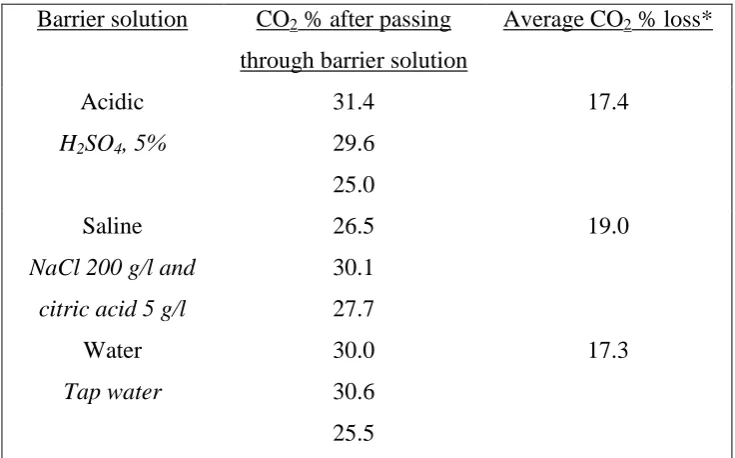
Table 3.6 The carbon dioxide loss depending on the barrier solution 106
Table 4.1 The description of tubes tested with varying seed fractions and substrate loading
117
Table 4.2 pH of food waste effluents at completion 127
Table 4.3 pH of effluents at completion for sucrose, cellulose and starch with variable organic loading rates
136
Table 4.4 Ratio of % methane/% carbon dioxide in the gas produced from cellulose degradation at varying OLRs
137
Table 4.5 pH of effluents at completion for rice with various loading rates 140
Table 4.6 Reproducibility of seed blanks used in testing of food waste (observed after 7 days incubation)
144
Table 4.7 Reproducibility of seed blanks used in testing of rice observed after 7 days incubation
144
Table 4.8 Chemical composition of the food waste sample 146
Table 4.9 Elemental composition of food waste in study by Zhang et al. (2003)
165
Table 5.1 Description of the continuous reactors 174
Table 5.2 The solid contents of the feedstock 175
Table 5.3 Description of Start-up trials 177
Table 5.4 Suggested thresholds for indicators of reactor stability 185
Table 5.5 The SCOD values corresponding to the methane percentages of a presumably healthy reactor
189
Table 5.6 Theoretical COD conversion factors for VFAs 192
Table 5.7 The FW2.6 reactor condition before and after treatments 195
Table 5.8 The meat reactor conditions before and after treatment 197
Table 6.1 Kinetics of 18.8 OLR of food waste in tubes after 20 days incubation
219
Table 6.2 The pH, experimental yield and volatile solids reduction of 18.8 OLR food waste digested in the tubes
225
vi 18.8 OLR food waste digested in the tubes
Table 6.4 Kinetics of 18.8 OLR food waste in 250 ml bottles after 20 days 228
Table 6.5 Comparison of reactor and effluent conditions after 20 days incubation for tubes and bottles digesting food waste
232
Table 6.6 The pH, experimental methane yield and volatile solids reduction of 18.8 OLR food waste digested in the bottles
233
Table 6.7 The value of k as a result of estimation using first order kinetics by varying the ultimate (B0) and specific (B) methane yield
235
Table 6.8 Kinetics of 11.0 OLR rice tested in tubes after 20 days 237
Table 6.9 The pH, experimental methane yield and volatile solids reduction of 11.0 OLR rice waste digested in the tubes
237
Table 6.10 Kinetics of 11.0 OLR rice tested in 250 ml bottles after 20 days 238
Table 6.11 The pH, experimental methane yield and volatile solids reduction of 11.0 OLR rice waste digested in the bottles
241
Table 6.12 Food waste digestion in batch and continuous reactors 242
Table 6.13 Rice digestion in tube and bottle and 11 g VS/L. d OLR 243
vii
LIST OF FIGURES
Figure 1.1 Anaerobic digestion described by the three processes 2
Figure 1.2 Outline of the cloning procedure for studying a microbial community
9
Figure 1.3 Schematic representation of DGGE 11
Figure 1.4 The in situ hybridization process described in four stages 12
Figure 1.5 Eudiometer unit 15
Figure 1.6 Supply of suitable substrates for anaerobic digestion 19
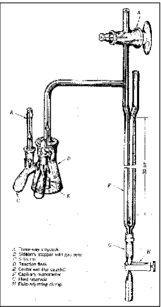
Figure 2.1 The Warburg apparatus 32
Figure 2.2 Schematic diagram of procedure for the anaerobic transfer of defined media into serum bottles
33
Figure 2.3 Experimental set-up for the dry anaerobic digestion experiments of the OFMSW
35
Figure 2.4 OxiTop Control AN6/AN12 for determination of anaerobic degradation process
36
Figure 2.5 Schematic description of the set-up of the BAM system 38
Figure 2.6 A simulated example for a substrate with B0 of 300 m3 CH4/kg VS 69
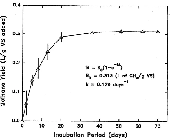
Figure 2.7 Typical biochemical methane potential curve of napiergrass 75
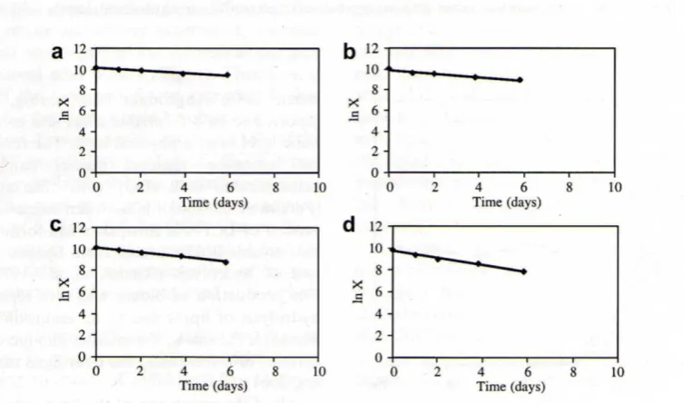
Figure 2.8 Linear plot of ln(X) versus initial time in the assays with an excess of (a) lipids, (b) cellulose, (c) protein and (d) carbohydrates
76
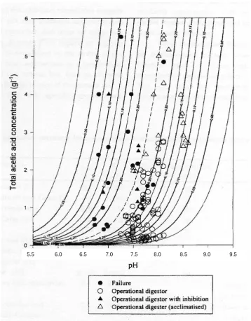
Figure 2.9 Contour plot showing effect of volatile fatty acid concentration and pH on specific microbial growth rate
79
Figure 3.1 The condition of food waste (a) once prepared, and (b) after blending for use in experiments
89
Figure 3.2 The meat substitute (a) made from pet food (b) as shown when cut and (c) sawdust which was sometimes added
90
Figure 3.3 The (a) cabbage (b) the prepared cabbage as continuous reactor feedstock
91
Figure 3.4 The rice as feedstock in the batch reactors 92
Figure 3.5 The tube during incubation 96
Figure 3.6 The parts and connections used in the tube 96
Figure 3.7 The 250 ml Schott bottles during incubation 97
Figure 3.8 (a) The continuous reactor during incubation, (b) the chute for inlet and outlet flow, and (c) the bung located inside the chute
98
Figure 3.9 The position of the PVC pipe in the 20 L continuous reactor 99
Figure 3.10 The mixing mechanism by manually rotating the reactor on an inclined shaker
99
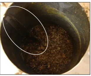
Figure 3.11 Baffled plate (marked by the oval shape) inside the continuous reactor for content mixing
viii
Figure 3.12 The gas analyzer when in use 101
Figure 3.13 Retention time of gas standards 103
Figure 3.14 The gas collection means (a) Tedlar bags (1 L and 5 L) for the batch systems and (b) helium balloons (13 L) for the continuous reactor
105
Figure 3.15 The (a) 500 ml and (b) 5 L water displacement devices 106
Figure 3.16 Retention time of VFA standards 110
Figure 3.17 The calibration curves for the individual VFAs 111
Figure 4.1 Illustration of biodegradation stages and methane generation 120
Figure 4.2 The tube design and operating procedure that was developed for measuring anaerobic decomposition of solid organic samples
123
Figure 4.3 Techniques to determine tube gas production 124
Figure 4.4 Accumulated methane production from food waste without the addition of seed or any supplements
124
Figure 4.5 The effect of organic loading rates of food waste on methane yields after (a) 6 days, (b) 20 days, and 34 days
126
Figure 4.6 Hydrogen progression against incubation time and methane percentage for food waste digestion at 18.8 OLR
128
Figure 4.7 Hydrogen progression against incubation time and methane percentage for food waste digestion at 25.1 OLR
128
Figure 4.8 Methane yields of food waste using seed from a laboratory operated reactor and from a wastewater treatment plant
129
Figure 4.9 Effect of different seed layers on methane percentage of food waste digestion
131
Figure 4.10 The methane yield of food waste from using 1, 4 and 14 days pre-digested seed in the batch test
133
Figure 4.11 The effect of seed pre-digestion on food waste methane production 135
Figure 4.12 Methane yield in response to different substrate of varied biodegradability and organic loading rate
136
Figure 4.13 The effect of substrate biodegradability and organic loading rate to its methane production after 16 days incubation
138
Figure 4.14 The methane yield of rice as a response to various OLR over time 139
Figure 4.15 The effect of organic loading rates on methane production of rice after (a) 4 and (b) 6 days of incubation
139
Figure 4.16 The methane yield in response to the (a) OLRs of different substrates after 6 days incubation and (b) effect on reactor pH
141
Figure 4.17 Methane yield from 10 replicates of food waste at 18.8 OLR conducted in one run
142
Figure 4.18 Methane yield of (a) food waste and (b) rice at OLR 50% and 75% of the maximum OLR
143
Figure 4.19 Methane production from 18.8 OLR of food waste over time 147
Figure 4.20 Daily gas production of the tubes corresponding to the ones marked ‘x’ in Figure 4.20, focusing from 20 to 59 days of incubation
ix Figure 4.21 The effect of mixing hourly compared to once a day mixing to
methane yield
149
Figure 4.22 The effect of reactor mixing on the methane yield of food waste when (a) mixed once a week at 18.8 OLR and (b) when not mixed (OLR of 14.4 g VS/L. d) throughout the incubation period
150
Figure 4.23 The effect of nutrient addition on methane potential of food waste 151
Figure 4.24 The response of food waste methane potential to the addition of nutrients
151
Figure 4.25 The effect of void reactor headspace on methane potential test of 18.8 OLR of food waste
153
Figure 4.26 The relationship between the reactor OLR to the VFA production and uptake as well as the methane production
161
Figure 5.1 The conditions of healthy reactors looking at VFA, alkalinity and pH of food waste digestion at (a) 2.6 OLR and (b) 5 OLR
179
Figure 5.2 Methane percentages of various substrates 180
Figure 5.3 The effluent conditions (pH, ammonia and soluble COD) from three reactors fed with substrate of different biodegradability; cabbage, food waste and meat
180
Figure 5.4 The methane percentage, pH, ammonia and soluble COD of meat mixed with sawdust reactor
181
Figure 5.5 Performance of reactors applying Start-up procedure 1 to 3 182
Figure 5.6 The pH trend of reactors FW7, FW5, FW3 and Start-up 1 during reactor start-up
182
Figure 5.7 The production of TVFA during the early days of continuous reactor operation
183
Figure 5.8 Performance of reactors using Start-up 4 184
Figure 5.9 Performance of reactors applying Start-up 5 184
Figure 5.10 (a) Relationship between CH4% and pH for different reactors (b)
pH decline for FW2.6
186
Figure 5.11 Relationship between NH3-N with (a) pH and (b) CH4% across
various reactors
187
Figure 5.12 Relationship between SCOD and (a) pH and (b) NH3-N for
different reactors
188
Figure 5.13 Relationship between propionic acid and pH for various reactors 190
Figure 5.14 The VFA and SCOD distribution in meat and sawdust, meat and FW5 reactors
191
Figure 5.15 Relationship between alkalinity to CH4% 193
Figure 5.16 The relationship between ammonia and carbon dioxide to alkalinity concentration in meat based reactors
193
Figure 5.17 Relationship between alkalinity and NH3-N across the many
reactors
194
Figure 5.18 The occurrence of washout after 100 days, and the methods to recover the FW2.6 reactor
196
x of reactor dilution
Figure 5.20 The decline of reactor performance due to temperature drop on Day 27, and the recovery following treatment
198
Figure 5.21 pH and alkalinity profile versus VFA concentration in the reaction medium
208
Figure 6.1 Cumulative probability graph of the estimated B0 values corresponding to Table 6.1
220
Figure 6.2 Cumulative probability of the estimated k values corresponding to B0 of 0.35 – 0.56 L CH4/g VS
220
Figure 6.3 The relationship between predicted ultimate methane yield (B0) and first order rate constant (k) for those results with estimated B0 between 0.35 -0.56
221
Figure 6.4 The relationship between predicted t lag and ultimate methane yield (B0) and first order rate constant (k)
222
Figure 6.5 Effect of the estimated B0 and k values if the t lag is assumed zero 222
Figure 6.6 Methane yield of 18.8 OLR food waste matching to Table 6.1 kinetic parameters inside ‘acceptable’ range
223
Figure 6.7 Methane yield of 18.8 OLR food waste to Table 6.1 with kinetics parameters out of ‘acceptable’ range
224
Figure 6.8 The distribution of B0, k and the sum of squared residual (SSR) for food waste at 18.8 OLR in the batch tubes
227
Figure 6.9 Cumulative probability graph of methane yield for 18.8 OLR food waste measured in the bottle after 20 days
229
Figure 6.10 Cumulative probability graph of rate constant for 18.8 OLR food waste measured in the bottle after 20 days
229
Figure 6.11 The relationship between estimated ultimate methane yield (B0) and first order rate constant (k)
230
Figure 6.12 The relationship between estimated t lag to ultimate methane yield (B0) and first order rate constant (k)
230
Figure 6.13 The distribution of B0, k and the sum of squared residual (SSR) for food waste at 18.8 OLR in the batch bottles
231
Figure 6.14 Methane yield of continuous reactor at 3 OLR food waste with 30 days HRT
234
Figure 6.15 Methane yield of continuous reactor at 1.5 OLR food waste with 30 days HRT
234
Figure 6.16 The relationship between k and B when different ultimate methane yield (B0) were applied
236
Figure 6.17 Cumulative probability graph of methane yield for 11 OLR rice measured in the 250 ml bottle after 20 days
238
Figure 6.18 Cumulative probability graph of first order rate constant for 11 OLR rice measured in the 250 ml bottle after 20 days
239
Figure 6.19 The relationship between estimated ultimate methane yield (B0) and first order rate constant (k)
239
Figure 6.20 The relationship between estimated t lag to ultimate methane yield (B0) and first order rate constant (k)
240
Figure 6.21 Comparison between the experimental and its estimated methane yield over time of 11 OLR rice digested in the bottles
241
xi the (b) corresponding OLR values
Figure 7.2 The determination of the ration of inoculums to substrate based on the VS% of sample
1
CHAPTER 1
INTRODUCTION
1.1 SUSTAINABLE MANAGEMENT OF WASTE THROUGH ANAEROBIC
DIGESTION
The challenge for the 21st century in terms of a sound waste management strategy is the transformation of waste into resources for the future (Lens et al., 2004). Utilization of
proper options for the treatment of organic wastes can turn this burden into an asset. One
way of achieving this is by employing biological waste treatment methods. Anaerobic
digestion is an example of an emerging method, offering avenues to recover both energy
through anaerobic process and compost whilst reducing waste at the same time.
Anaerobic digestion is the biological decomposition of organic substrates in the absence
of oxygen. In anaerobic treatment, its benefits, advantages, limitations and requirements,
which are unique to each substrate, are often dictated by its biodegradability.
Understanding substrate biodegradability hence becomes important when designing or
operating a waste treatment plant. Certain operating parameters such as temperature or
mixing and substrate related factors like loading rate and pretreatments may be better
suited than others and this might form a logical limit on the usefulness of a given
approach. In response to this question, research at laboratory level is usually conducted
beforehand to pinpoint suitable operating conditions and foresee any technical or toxicity
issues with a waste sample.
1.2 AN OVERVIEW OF THE ANAEROBIC DIGESTION PROCESS
When an organic material enters into a digester, it contains a large fraction of suspended
2 molecules are converted, mainly, into methane (CH4) and carbon dioxide (CO2) by the
action of bacteria. The overall biochemical reaction can generally be simplified to:
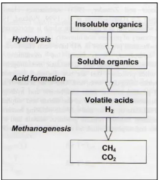
The process of anaerobic digestion proceeds in three main stages; (i) hydrolysis, (ii) acid
[image:22.612.225.387.235.418.2]formation and (iii) methanogenesis (refer Figure 1.1).
Figure 1.1 Anaerobic digestion described by three processes
(source: Mata-Alvarez, 2003)
1.2.1 Hydrolysis
Hydrolysis is the first step in the anaerobic biodegradation process. It involves the
conversion of the complex waste (particulate and soluble polymers) into soluble products
by the extracellular enzymes secreted by the hydrolytic bacteria. The once complex
insoluble organic polymers become more easily available for use by the acidogenic
bacteria in the next stage. Proteins present in the waste are converted into amino acids,
fats into long chain fatty acids and carbohydrates into simple sugars.
Hydrolysis has been reported to usually be the rate-limiting step, since bacterial action at
this stage proceeds slower than the other following digestion steps. Substrate availability, Organic material CH4 +CO2 +H2 +NH3 +H2S
3 bacterial population density, temperature and pH (Chynoweth and Isaacson, 1987;
Palmisano and Barlaz, 1996; Evans, 2001) all affect the rate at which hydrolysis
proceeds. The competence of the hydrolysis stage plays a huge role in determining the
substrate ultimate methane yield. A municipal solid waste (MSW) for example only
underwent 50% hydrolyzation of its organic matter, while the rest remained undegraded.
This phenomenon occurred because certain sites within the solid matrix are inaccessible
to the hydrolysis enzymes and due to shortage of appropriate organisms secreting the
necessary extracellular enzymes (Palmisano and Barlaz, 1996).
1.2.2 Acid formation
1.2.2.1 Acidogenesis
In acidogenesis, the organic monomers of sugars and amino acids released earlier are
degraded by the fermentative bacteria to produce volatile fatty acids (VFA) namely
propionic, butyric and valeric acids, together with acetate, hydrogen (H2) carbon dioxide
(CO2). The degradation of amino acids also produces ammonia (NH3).
1.2.2.2 Acetogenesis
During the acetogenesis step, the obligate hydrogen producing acetogens (OHPA) break
down both long chain fatty acids (LCFA) and volatile fatty acids (VFAs), producing
acetate, carbon dioxide and hydrogen. LCFA are organic acids having more than 5 atoms
of carbon (Angelidaki et al., 1998). Carbon dioxide is produced when fatty acids as
electron donors degrades, at the same time, as electron acceptors, transforming H+ into H2
(Mata-Alvarez, 2003).
1.2.3 Methanogenesis
Methane is produced from the raw materials of the previous stage during the
methanogenesis stage. This is done via two ways; one through hydrogenotrophic
methanogenesis producing methane by utilizing H2 and CO2 by the hydrogen-consuming
4 aceticlastic bacteria which grow on acetate as substrate, releasing methane and carbon
dioxide. Of these, acetic acid (CH3COOH ) and the closely related acetate are the main
precursors to methane production accounting to about 75% of the methane production, as
depicted in the following equation:
CH3COOH CH4+CO2
Methane forming bacteria may also use methanol:
CH3OH+H2 CH4+H2O
or carbon dioxide and hydrogen:
CO2+4H2 CH4+2H2O
Source: Evans, 2001
The evolution of the biogas coincides with the cellulose decomposition and is better
illustrated with curves going through five main phases, as described below (source:
Evans, 2001):
Phase I
Maximum cellulose loadings; oxygen content drops to near zero; carbon dioxide at
atmospheric levels (78%)
Phase II
Carbon dioxide, hydrogen and free fatty acids levels rise to peak values; cellulose
breakdown begins
Phase III
Carbon dioxide decreases to plateau at around 40%; methane production commences and
achieves plateau at around 60%; free fatty acids decrease to hold at minimal levels;
cellulose breakdown continues at a linear rate with respect to time
5 Plateau phase with carbon dioxide at circa 40% methane at circa 60% and free fatty acids
at less than 5%; cellulose declines steadily throughout this phase
Phase V
Cellulose becomes fully decomposed, resulting in the tail off to zero of methane and
carbon dioxide; oxygen regain atmospheric levels (20%).
1.2.4 Process balance
When the rate of hydrolytic and fermentative activity exceeds the rate of acetogenic
conversion of fermentation intermediates, process inhibition occurs since methanogens
cannot consume dihydrogen at the rate at which it is produced. When methanogenesis is
inhibited, electron or hydrogen accumulates. This results in the formation of various other
fermentation products like propionate, butyrate, lactate, succinate, and alcohols, wanting
to rid of the electrons or hydrogen. The reactor pH then decreases as the levels of this
fermentation products continue rising. The methane forming bacteria are pH sensitive and
can only usually tolerate more or less neutral pH values of between 6.5 to 7.5.
If the fermentation products accumulate to inhibitory levels, the decomposition of
substrate will cease. It is therefore very important to understand that the overall
fermentation is dependent largely on the particular bacteria species present and to a lesser
extent its environmental conditions. There has to be a balance between activities of
bacteria that form organic acids, carbon dioxide, and dihydrogen (or formate) and the
methanogenic bacteria which utilize these substrates. By changing VFAs into methane
and other related gasses, any inclination towards an augmentation in VFA concentration
which simultaneously decreased the digester pH, is removed. The acid/base equilibrium
is hereby naturally regulated, removing the likelihood for biochemical inhibition and/or
6 1.2.5 Kinetics
The three major anaerobic degradation processes described earlier, namely the
hydrolysis, acidogenesis/acetogenesis and methanogenesis can be modelled, providing
theoretical understanding of the microbial populations and their interactions in the
environment within the reactor. Not only can the reactor design and operation be
optimised, the kinetic equation is particularly useful as guidelines for scale-up of the
digestion systems.
For different substrates, the kinetics are different; and for each substrate the kinetics vary
with operating conditions. Numerous kinetic models have been developed to describe the
degradation steps involved such as Monod, Step Diffusion, Inhibition and Shrinking Core
(Chynoweth and Isaacson, 1987; Mata-Alvarez, 2003). The simplest rate expression is
the first-order kinetic model since only a single parameter needs to be estimated.
Although sometimes limited, especially where complex substrate and systems are
involved, the first-order model is generally capable at predicting the anaerobic process
with a great degree of reliability. Considering the importance of process kinetics to this
research as well as the vast information the topic itself carries, it seems more appropriate
to conduct a thorough review. Further description and discussion of the biodegradation
yields and kinetics as an essential tool for rational reactor design is allocated in Chapter
2: Literature review.
1.3 MEASURING ANAEROBIC DECOMPOSITION
Anaerobic biodegradability can be ascertained by the amount of substrate transformed or
the intermediates and end products developed by the different microorganisms groups.
The volume of biogas produced also gives an indication of anaerobic decomposition. A
number of methods are available to measure anaerobic biodegradability. Although these
techniques vary in terms of the test procedure, measuring system and results, they can
7 equipment used to measure anaerobic biodegradability and activity including those that
use (i) a variety of chemical analysis techniques to quantify substrate depletion or the
formation of intermediates and end products, and (ii) microbiological based methods and
(iii) gasometric measurement techniques to measure the amount of biogas produced.
1.3.1 Analysis of substrate consumption or product formation
1.3.1.1 COD, TOC, DOC
Substrate concentrations can be quantified by using either a summary or a
substrate-specific parameter. The dissolved organic carbon (DOC), chemical oxygen demand
(COD) and total organic carbon (TOC) are generally applicable to assess the
consumption of the whole substrate. However, the evolution from one component to
another by anaerobic biodegradation may affect only a small change in COD, TOC or
DOC, making the change harder to detect. Moreover, the complex nature of the test
sludge and the tendency of some test chemicals to absorb to sludge particulate material
may upset the suitability of the method to monitor substrate conversion (Birch et. al.,
1989). That said, this does not mean that these gross measurements (as well as volatile
solids, VS) are incapable of telling when there is substrate conversion to gas (CO2/CH4).
1.3.1.2 Uniformly 14C labeled test substances
In the investigation of benzene degradation by Burland and Edwards (1999),
radioactively labeled 14C was used and monitored by scintillation counting of radioactivity. The 13C-labelled and 14C-labelled substances have also been followed using gas chromatography-mass spectrometry (GC-MS) as a way of quantifying the mass
balance between substrate and products (Dolfing and Bloemen, 1985). Tests using these
radioactively labeled substances involve the detection of radioactive methane and carbon
dioxide to present clear indication of ultimate biodegradation. While this test is well
validated, the labeling approaches of its test procedure limits the test’s widespread
applicability, especially when screening new chemicals. Labelling approaches involve
8 Another approach is to employ 13C-labelled substrates produced by organic synthesis. A wide range of 13C-labelled compounds are available from commercial suppliers. The 13 C-labelled synthetic compounds can be expensive, thereby restricting their use in field scale
studies (Evershed et al, 2006).
1.3.1.3 Coenzyme F420
Methanogens induce UV blue-green autofluorescence, quantifiable under an
autofluorescence microscopy. Methanogens with a high content of F420 such as the
hydrogen-utilising methanogens are visible. Exceptions apply to some methanogens
which are not visually clear such as the acetate-utilising methanogens that cannot be
counted at all or the genus Methanosarcina which are found in clumps made of many individual cells (Solera et al., 2001a).
A high correlation was evident between the methane production and methanogenic
population in thermophilic anaerobic reactors using autofluorescence microscopy as the
method of analysis (Solera et al., 2001b). This method benefits over traditional
microbiological methods as it can provide predictive value of the sample’s potential
methanogenic activity without the need for culturing. A later study by Demirel and
Yenigun (2006) found that numbers of autofluorescent methanogens decreased during
start-up. The type of substrate used and/or the variations of the organic loading rate
(OLR) may have affected the morphology of the autofluorescent methanogens during
start-up.
The technique is not capable for distinguishing between live and dead microorganisms. In
addition, the accuracy of results is easily influenced by fading of the autofluorescent cells
and the presence of weakly or non-fluorescent cells (Solera et al., 2001a).
1.3.2 Analysis based on microbiological methods
The molecular biology approach is based on the RNA of the small ribosomal subunit (S
9 to its obvious advantages, namely (i) being universal and abundant in all living beings
(103 to 105 ribosomes/cell) (ii) molecule highly preserved throughout evolution (iii) sufficiently long gene sequence to produce statistically relevant data and (iv) gene can be
easily sequenced with current technology (Sanz and Kochling, 2007). The current
techniques most widely used include cloning of 16S rDNA, denaturant gradient gel
electrophoresis (DGGE) and Fluorescent in situ hybridization (FISH).
1.3.2.1 Cloning of 16S rDNA
Cloning and sequencing for 16S rDNA is the most widely used procedure in molecular
biology. The technique involves nucleic acids extraction, then magnification and cloning
of the 16S rDNA genes. The genes are later sequenced and the isolated clone identified
using phylogenetic software (Figure 1.2).
Figure 1.2. Outline of the cloning procedure for studying a microbial community
(source: Sanz and Kochling, 2007)
Mladenovska et al., (2003) was able to identify the microbial communities affecting the
performance of two anaerobic reactors treating cattle manure and a mixture of cattle
10 that archaeal species were restricted in both reactors with most clones related to the
Methanosarcina sicilae. Presence of sequences related to the species Methanosarcina sicilae in both reactors indicated that the same acetate-utilizing methanogens were active in conversion of higher amounts of acetate generated during the degradation of LCFA.
The cloning approach was also applied to characterize the microbial properties of a
methanogenic granular phenol-degrading sludge in the work by Zhang et al. (2005).
Together with FISH, a detailed picture of the microbial population especially the species
responsible for phenol degradation was better identified.
Cloning of 16S rDNA yields far more exact phylogenetic information than other
molecular techniques such as FISH and DGGE, however, it is less accepted in the fields
of environmental engineering. Demands for specialized personnel and equipment not
necessarily available in engineering and chemistry departments may be the reason behind
this lack of popularity. The cloning method also can be time consuming and
cumbersome, making it unpractical for high sample thoroughput (Sanz and Kochling,
2007).
1.3.2.2 Denaturant gradient gel electrophoresis (DGGE)
Denaturant gradient gel electrophoresis (DGGE) helps determine the dominant members
of a microbial community with the medium phylogenetic resolution without having to go
through a laborious method as the cloning of 16S rDNA. This is generally so if
knowledge of the exact phylogenetic information is less desirable.
With the DGGE technique, band patterns that directly reflect the genetic biodiversity of
the sample are generated, following the various mobility on a gel of denatured
DNA-fragments of similar size but with different nucleic acid sequences. The procedure is
described in Figure 1.3.
When DGGE analysis was used for studying the effect of various dilution rates on
carbohydrate fermentation in a continuous flow stirred tank reactor, a population shift in
11 exposed. Majority of the microorganisms population detected were that of closely related
thermophilic anaerobic bacteria. Another study demonstrated the applicability of DGGE
for showing impact of temperature on bacterial community structure and diversity for
bioreactors treating pharmaceutical wastewaters (Lapara et al., 2000). Three distinct
microbial communities were observed with a reduction in number of bacterial
populations seen under elevated, thermophilic reactor temperature.
Figure 1.3 Schematic representation of DGGE (source: Sanz and Kochling, 2007)
The DGGE technique is very valuable for following dynamic modification in microbial
communities, especially involving a large number of samples. It allows a rapid and
simple examination of band patterns. However, the small number of detected bands
restricts the number of identifiable species. The phylogenetic relations are thus less
reliable, since the sequences of the bands involve only a small region (200-600 bp) of the
12 1.3.2.3 Fluorescence in situ hybridisation (FISH)
Fluorescence in situ hybridisation (FISH) is a technique that uses fluorescently labeled phylogenetic oligonucleotide hybridisation probes to detect specific microbial groups.
The microbial cells having 16S rRNA sequences are hybridized with the fluorescent-dye
labeled probes and detected under a microscope. The microbial abundance and/or activity
are determined from the extent of hybridization (Figure 1.4).
Figure 1.4 The in situ hybridization process described in four stages
(Sanz and Kochling, 2007)
Stahl et al. (1995) have earlier distinguished probes suitable for identifying methanogenic
microorganisms at different taxonomic levels (order, family and genus). Their work sets
the ground for further application of FISH in the area of anaerobic digestion. Such
applications include the determination of methanogenic activity in thermophilic-dry
anaerobic reactors by comparing the amount of methane generated with the size of
methanogenic population (Montero et al., 2008). The capability of FISH to illustrate the
13 has also been verified (Calli et al., 2005). The propionate degrading acetogenic bacteria
were more sensitive to free ammonia than methanogenic archea.
The test itself is suitable for routine analysis as it is fast and easy to perform without use
of highly trained and specialized personnel. However, problems may arise if the probe for
the desired bacterial taxon or group is not available. In addition, the user needs to be
familiar with the target microorganisms, its ecosystem and the rRNA sequence is
necessary prior to using FISH technique.
1.3.3 Gasometric measurement techniques
The gasometric methods, or sometimes termed respirometer, have been repeatedly
applied for determining anaerobic biodegradation (Birch et al., 1989; Colleran et al.,
1992; Guwy, 2004). Gasometric methods incorporate a simple apparatus: (i) the reactor
and its associated contents and (ii) gas quantification system to determine the amount of
biogas produced as a result of microbial activity in a given sample.
1.3.3.1 The reactor
The most common reactor configurations for anaerobic degradability testing in the
laboratory are the batch and continuous type. The reactors differ in terms of their feeding
modes, effluent analysis, test period as well as the kinetics, and are generally chosen
depending on the objective of the study.
In the batch approach, the substrate is incubated with inoculum and may be supplemented
with a buffer solution and nutrients. The batch operation is characterized by no addition
to and withdrawal from the reactor after initiation until the end of the incubation period.
If the reactor effluent needs to be analysed over time, a system where several reactors is
used is usually the most suitable option. Several identical reactors are set-up at the start
and assumed to represent one large reactor undergoing similar biodegradation process
14 The continuous set-up uses stirred tank reactors with analysis made on the effluent once
steady state is established. Here, nutrients essential for growth are continuously fed. A
portion of the reactor contents is continuously withdrawn and exchanged with equivalent
amount of fresh substrate.
The continuous procedures closely simulate full-scale anaerobic operation; however, they
are costly in terms of facilities, equipment, time and personnel. Long term operation of
continuous processes are prone to many operating difficulties, such as contamination and
cell washout causing decrease in activity. It is also susceptible to unanticipated
disturbances like temperature failure and feedstock variability. The batch operation is not
restricted by the same weaknesses as the continuous reactors. Batch procedure allows the
evaluation of a wide range of variables; however, there is still room for further
improvement. The advantages, flexibility, capabilities and kinetics of each reactor
configuration in realising anaerobic biodegradation potential of solid organic waste is
examined even more in the succeeding chapter (Chapter 2: Literature review).
1.3.3.2 Gas quantification system
The volume of biogas generated is determined either through volumetric or manometric means. The former measures the biogas volume by keeping the pressure constant while
the latter measures the pressure increase by keeping the volume constant.
a) Volumetric methods
In volumetric methods, the biogas produced is allowed to move into an external
collection system that measures the volume produced. This may be as simple as a
lubricated glass syringe that is inverted straight onto the lid of the reactor, first
introduced by Owen et al. in 1979. The overpressure generated inside the reactor forces
the piston to expand, balancing the pressure buildup to atmospheric pressure. The volume
of biogas is read off straight and then either injected back into the serum bottle, or
15 Alternatively, liquid displacement device can be employed. The set-up usually consists of
a suitable vessel filled with a barrier solution and inverted in a reservoir. The biogas from
the reactor passes to this liquid filled vessel thus displacing an equivalent liquid volume.
The amount of biogas is determined either by graduation or by weighing the weight of
liquid displaced.
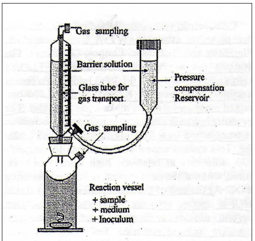
The Eudiometer unit is a standardized example of a manual volumetric method based on
the liquid displacement concept (see Figure 1.5). Reading is taken off the graduated gas
collecting tube, after the barrier solution is displaced into the reservoir tank. To bring the
displaced liquid to its original level (liquid levels in both the gas collecting tube and the
reservoir tank are similar), the reservoir tank is raised so that the biogas returns to
[image:35.612.179.434.338.579.2]atmospheric pressure.
Figure 1.5 Eudiometer unit (adapted from Guwy, 2004)
Most of the above mentioned techniques can be run automatically. The automation
usually relies on the container reaching a pre-set level which will then activate a sensor.
This sensor then triggers a solenoid valve (two way or three way), releasing the
16 counter rotates or ticks to account for one unit volume of gas produced. The cycle will
repeat itself thus begins another count. Recent example of this automated liquid
displacement concept utilizes a volumetric cell for gas-liquid displacement and optical
couplers as sensors for liquid level detection (Liu et al, 2004). An alternative design
prefers gas accumulation which is regulated by a counter-weighted floating cap and the
level controlled by a pressure sensor (Smith and Stockle, 2008). Kuss and Young (1992)
invented a bubble counter, where gas bubbles of very small volumes of gas passed
through a photocell and a detector count the number of bubbles formed. These new
inventions are a result of ongoing modifications from previous developed devices such as
the ones used by Cooney (2006), Glauser et al. (1984), Gwatkin et al. (1986), Liu et al.
(2004) and Veiga et al. (1990). The vast number of gas measurement designs points out
that no single device is suitable for all researchers governed by the availability of local
supplies, funding and the research requirements.
b) Manometric Methods
Under manometric means, the pressure build up is measured from the biogas being
confined in the reactor itself. Pressure increase can be traditionally measured using a
differential manometer, however the work by Shelton and Tiedje (1984) sets the ground
for applicability of pressure transducers in quantifying biogas production. Pressure
transducers have been widely accepted ever since as they can be installed within the
reactor, allow easy automation and amenability to computer control.
Various configurations of the pressure transducer techniques are available. Generally, the
set-up depends on the pressure inside the reactor reaching a set value and sending an
electric signal to a control interface that activates a three-way solenoid valve. The second
valve will shut to maintain the internal pressure of the reactor while the third valve will
open to release excess pressure to the atmosphere. After a set time period (about 3
seconds), the valve will deactivate and a new cycle begins. The system employed by Ince
et al. (1995) incorporates the use of a microcomputer which enabled monitoring of 8
independent reactors simultaneously. Coates et al. (1996) used a portable pressure
17 found the method to be comparable with the conventional gas chromatographic
measurement of the biogas composition. Angelidaki et al. (1998) also described a
computerized system simultaneously monitoring 16 reactors with the results validated
against a gas chromatographic analysis.
The water displacement devices which make up the majority of volumetric gas metering
methods are cheap and involve simple laboratory apparatus like water cylinders and
plastic tubings. The manual approach is often cumbersome and time consuming making
extended incubation period harder. This is due to the need for constant evacuation and
resetting of the water level as large gas volumes cannot be catered by the small reservoir
liquid available for the volume displacement. The automatic approach is less labour
intensive but is more prone to problems associated with reservoir levels, corrosion, and
complexity in managing CO2 solubility and algae growth (Guwy, 2004). Corrosion is
especially an issue with electronic solenoid valves and may be lessened using a siphon
valve instead. The bubble counter is easily influenced by the liquid volume and viscosity
where any variation may affect the bubble size thus the volume measured.
The pressure transducer can yield very accurate output and is easier to perform than the
liquid displacement techniques, although more effort is required in its initial set-up.
However, the technique is more susceptible to pressure rise with the temperature and
gas-to-liquid volume ratio highly influencing the measurement. Temperature deviations may
cause background fluctuations, decreasing the sensitivity of a pressure transducer. On the
other hand, the sensitivity of the technique is enhanced when a low gas-to-liquid volume
meaning a reduced headspace volume is opted.
Regardless of which gasometric method, whether volumetric or manometric, the
dissolution of CO2 into water and its effects to the measurement is a recurring
phenomenon. It is widely accepted that a considerable fraction of carbon dioxide can
dissolve in water while methane hardly does. Factors such as pressure, pH, ratio of
headspace-to-liquid volume, temperature and the complex thermodynamic equilibria
18 magnesium determines the solubility of CO2. To reduce errors associated with CO2
solubility, large increase of pressure should be avoided and can be done by venting the
accumulated gas regularly. Another option is through use of a suitable barrier solution
such as highly acidic or saline to avoid CO2 diffusion in the liquid. An alkaline solution is
an alternative if only methane needs to be measured since all the carbon dioxide in the off
gas will be absorbed.
1.3.4 Summary of anaerobic biodegradability tests
This section has outlined the existing methods for measuring anaerobic biodegradability
which builds upon chemical analysis techniques (e.g. COD, TOC, DOC; 14C labeled substrate; Coenzyme F420), microbiological based methods (16S rDNA; DGGE; FISH)
and gasometric measurement techniques (volumetric and manometric).As pointed out
earlier, these methods differ from each other in a variety of ways. The procedures,
materials, detection systems and output differs considerably thus the method of choice is
up to the researcher to decide.
However, in the field of environmental technology the gasometric measurement
techniques are generally preferred due to the information that is obtainable with the
method as well as the availability of laboratory equipment and knowledge. The demands
for sophisticated technology and equipment along with requirement of microbiological
knowledge with the other analytical methods limit their applicability across
environmental engineering research. Based on this logic this research will be focusing on
the gasometric approach for measuring anaerobic decomposition, and improvements for
the current technique will be recommended.
1.4 ANAEROBIC DIGESTION FEEDSTOCK
19 The development of anaerobic digestion was primarily to care for liquid wastes with or
without suspended solids, such as domestic or industrial wastewaters, manures and
sludges from biological or physic-chemical treatments, among others. In the recent years,
increased environmental awareness, coupled with the demand for sustainable waste
management strategies and renewable energy form, has widened the application for
anaerobic digestion. Organic waste diversion from landfills including domestic and
industrial organic wastes has gained growing recognition locally and internationally. It is
a move that is motivated towards reducing diverse impacts on the environment such as
emanating odours, attracting vermin, emitting toxic gases, contaminating groundwater
and wasting landfill capacity. Figure 1.6 summarizes the variety of feedstock used in
anaerobic digestion system.
Figure 1.6 Supply of suitable substrates for anaerobic digestion
1.4.1.1 Agricultural waste
Among the agricultural wastes, pig and cow slurry, chicken manure and farmyard manure
are of primary concern because of the detrimental effect on the environment. The natural
degradation of livestock wastes during storage leads to a release of greenhouse gases
(CH4 and CO2) to the atmosphere due to the anaerobic decomposition of the organic
matter (Vedrenne et al., 2008). In addition, an improper application of animal manure
containing nitrogen and phosphorous to land can result in eutrophication of surface waste
ANAEROBIC
DIGESTION
AGRICULTURAL WASTE
INDUSTRIAL WASTE AND WASTEWATER
ENERGY CROPS
MUNICIPAL ORGANIC
20 resources and pollution of soil and groundwater (Gungor-Demirci and Demirer, 2004).
Anaerobic digestion has been used in a beneficial way to treat and dispose of the
livestock waste by making use of its methane potential. The methane potential of manure
comes from the digestion of the organic components in the faeces and in the straw used
as bedding material, which is mainly: carbohydrates, proteins and lipids (Moller et al.,
2004).
Studies by Gungor-Demirci and Demirer (2004), Kaparaju et al. (2008), Vedrenne et al.
(2008), Moller et al. (2004), Kaparaju and Rintala (2008) and Samy (2000) have shown
that the by-product of cattle, poultry, and swine are suitable as feedstocks for anaerobic
digestion. The methane potential for pig can be expected to be between 0.244 – 0.343 L
CH4/g VS while sows are from 0.260 – 0.334 L CH4/g VS. The average methane
potential from dairy cattle slurries is estimated at 0.243 + 0.041 L CH4/g VS and is
usually lower than the average methane potential from swine slurries at 0.297 + 0.040 L
CH4/g VS. The methane yield from calves and duck slurries are 0.386 and 0.319 L CH4/g
VS, respectively (Vedrenne et al., 2008).
The methane potential of livestock waste is influenced by the different organic matter
compositions related to animals diet (Vedrenne et al., 2008). Cattle are fed with roughage
which contains greater amounts of lignin and cellulose than pig feed does. Furthermore,
the amounts of proteins and lipids are considerably higher in pig than cattle manure. Due
to the higher proportion of lipid in pig manure, theoretically, the methane would be
higher in both pig and sow manure than in cattle manure (Moller et al., 2004). The
amount and type of bedding material also affects the methane productivity of the
livestock waste. The use of straw as bedding material (10 g straw per 1 kg manure) has
been found to increase the methane yield of the manure by 10% (Moller et al., 2004).
1.4.1.2 Energy crops
Cultivation of crops specifically for anaerobic digestion purposes could be of interest for
countries where energy costs are high and where sufficient agricultural land is available.
21 between 0.211 L CH4/g VS (Raposo et al., 2006) to 0.300 L CH4/g VS (Pereira et al.,
2009). Chynoweth et al. (1993) when investigating the methane potential of several
biomasses, found methane values were low with crops containing more lignin or the
presence of inhibitors (e.g. tannins and resins in soft woods). Methane yield increased
with harvest frequency especially for napiergrass, and that methane is generally higher in
leaves than in stems. The study by Chynoweth et al. (1993) also found that post-harvest
conditions such as ensiling or drying did not have a significant influence on methane
yields. Although the production of energy crops for the purpose of producing bio-oil has
been proven viable, its full scale adoption is still yet to be well accepted. Continuing
argument exists over the importance of land use for human consumption over energy
production, especially for areas where arable lands are scarce.
1.4.1.3 Industrial waste and wastewater
Huge amounts of agricultural raw materials like plants and livestock are processed in the
food industries. During processing, wastes and wastewater are produced which are
typically high in organic matter, making these waste products feasible feedstock for
anaerobic digestion. Some examples include wastewater from soybean (Yu et al., 1998)
and orange juice (Siles et al., 2007) processing and spent apples from producing apple
juice (Frederic et al., 2007). The meat processing industry emits grease trap sludge which
are lipid rich, have small fibrous structure and high water content (Luste et al., 2009).
Lipids have high methane production potential but when excessive, can be inhibitive due
to the production of long chain fatty acids (LCFAs). The digestive tract content comprise
of partly digested fodder high in carbohydrate and lignin, which could be resistant to
anaerobic breakdown. The effluent generated during the unloading of fish from ships is
also high in organic load. The wastewater produced from the fishmeal industry contains
elevated sulphide and sodium, however has been shown susceptible for anaerobic
treatment provided a suitable adapted inoculum is used (Aspe et al., 1997). One of the
drawbacks with most food processing industries as anaerobic digestion feedstock is the
seasonal feed variation having an effect on the quality and quantity of gas production.
This is because the availability and demand for particular product changes considerably