Application of graph theoretical methods to the functional connectome of human brain

(1)

warwick.ac.uk/lib-publications

A Thesis Submitted for the Degree of PhD at the University of Warwick

Permanent WRAP URL:

http://wrap.warwick.ac.uk/88528

Copyright and reuse:

This thesis is made available online and is protected by original copyright.

Please scroll down to view the document itself.

Please refer to the repository record for this item for information to help you to cite it.

Our policy information is available from the repository home page.

(2)

Application of Graph Theoretical Methods to The

Functional Connectome of Human Brain

by

Soroosh Afyouni

Thesis

Submitted to the University of Warwick

for the degree of

Doctor of Philosophy

Institute of Digital Healthcare

(3)

List of Tables

3.1 Porportion of nodes in each module that contributes to the RC organisation

of healthy subjects . . . 50

3.2 Porportion of nodes in each module that contributes to the RC organisation

of Schizophrenic subjects . . . 50

5.1 Disruption indices, as discussed in section 3.1.10, of RSNs of three atlases

(Power2011, AAL2 and Yeo17) for the NoGSR case of local measures in

Statistical Thresholding. . . 118

Statistical Thresholding. . . 119

(Power2011, AAL2 and Yeo17) for the GSR case of local measures in

Den-sity Thresholding. . . 126

Density Thresholding. . . 127

B.1 List of blocks and the percentage that each anatomical region participated

(8)

List of Figures

2.1 A.Headline of the NYT report regarding the Moreno’s presentation

(Cour-tesy of The New York Times). B.Network of blog-to-blog interaction in

2004 US election. Red nodes represent pro-democrat blogs and blue nodes

represent pro-republican blogs. Reproduced from Adamic and Glance (2005) 11

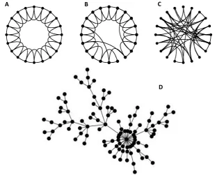
2.2 A.a lattice network with Dirac Delta degree distribution B.a smallworld

network (SW model). C.a random network with Poisson degree

distribu-tion (ER model)D.a Scale-Free network with power-law degree distribu-tion (BA model). Reproduced from Watts and Strogatz (1998) and Barab´asi

et al.(2009).. . . 14

2.3 Cartoon presentation of a small-world network, with modular structure and a strongly connected core which mediates the modules. Reproduced from

Bullmore and Sporns (2012a). . . 15

2.4 Google Trends representing the interest in the topic ’connectome’ over a

period of 12 years (Jan 2004 - Aug 2016). Spikes (shocks) in the search

trend are marked with a brief description. . . 16

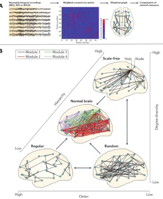
2.5 A. Common procedure for constructing the functional connectome. B.

Topological description of the human brain, suggesting the human

connec-tome is located between three topological extremes (random, lattice and

scale-free). Reproduced from Stam (2014) . . . 18

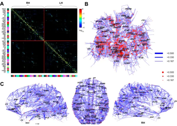
2.6 Hagmann et al 2008 description of structural connectome: A.Adjacency

matrix of the structural connectome of healthy brains. B.Topological pre-sentation of nodes configured based on Kamada-Kawai force-spring layout

C.Spatial reconfiguration of figure B with brain region coordinates. Repro-duced from Hagmannet al.(2008) . . . 20

(9)

3.2 Projections of edges that were found to be significantly decreased during

schizophrenia by NBS. Results the NBS over different thresholds were

shown in each panel. . . 36

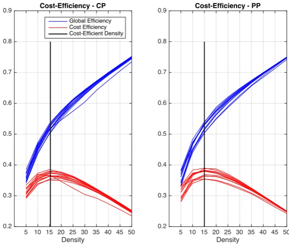
3.3 Cost efficiency of brain networks in Healthy (Left) and Schizophrenic (Right).

Global efficiency of each subject is shown in blue and cost-efficiency is shown in red. The mean cost-efficient density for each group is shown with a vertical black line. . . 37

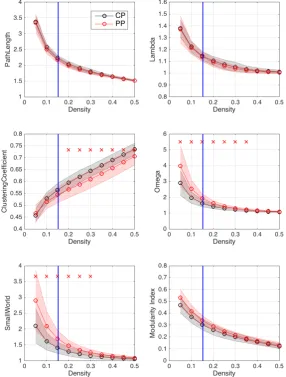
3.4 Global measures of segregation, integration and complexity. Panel A. shows

the global measures for the level of integration: path length (Left) and nor-malised path length (Right). Panel B. shows global measures for segre-gation: clustering coefficient (Left) and normalised clustering coefficient (Right) and maximised modularity index (Bottom) Panel C. shows the small-world index as a measure of complexity . . . 40

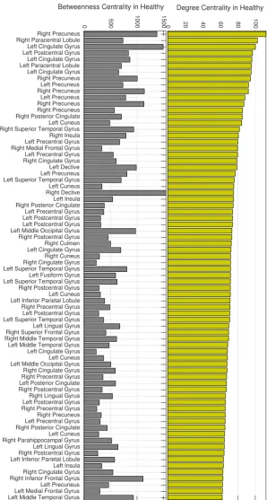
3.5 Degree (top) and betweenness (bottom) centrality for averaged across healthy

subjects. . . 42

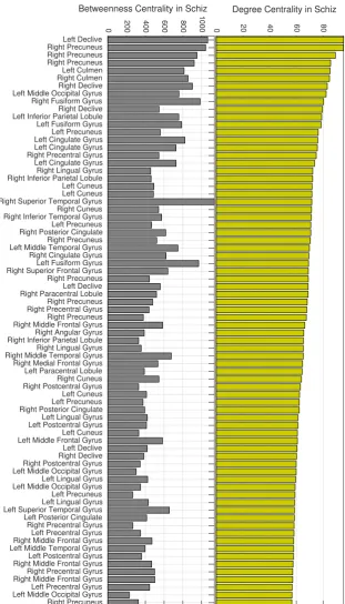
3.6 Degree (top) and betweenness (bottom) centrality for averaged across Schiz

subjects. . . 43

3.7 Disruption plots of Degree centrality (Left), Betweenness centrality

(Mid-dle) and Local Efficiency (Right) . . . 44

3.8 A. Modularity index across different scales for both empirical and

ran-domised networks in healthy (Left). Module configurations on re-arranged

group-averaged network of healthy (Right).B.Modularity index across dif-ferent scales for both empirical and randomised networks in schizophrenia (Left). Module configurations on re-arranged group-averaged network of

schizophrenia (Right).. . . 46

3.9 Projection of individual nodes and their module assignments on a transpar-ent surface of the human brain. . . 47

3.10 A river-plot shows the overlap between modular structure of healthy and

schizophrenia subjects. . . 48

3.11 Similarity between node assignments of modularity algorithm across

sub-jects of healthy (Left) and schizophrenia (Right) . . . 49

(10)

3.13 Interaction between RC organisation and rest of the network via feeder and

local connections. A. Analysis of density between feeder, local and RC

nodes as well as between healthy and schizophrenia subjects. B.

Analy-sis of Local efficiency of local, feeder and RC nodes as well as between

two groups. C.Analysis of Betweenness Centrality of feeder, local and RC nodes. Red asterisks indicate significant differences.. . . 52

3.14 NRCC of healthy (Top) and schizophrenia (Bottom), as decribed in section 3.1.9. Nodes that were identified as significantly different were marked with a red asterisk . . . 53

3.15 NRCI of healthy (Top) and schizophrenia (Bottom), as decribed in section 3.1.9. Nodes which were identified as significantly different were marked with a red asterisk . . . 54

3.16 Similarity between Rich Club Identity matrices across individuals across

healthy (Left) and schizophrenia (Right) . . . 55

4.1 Rich Block detection procedure on a toy connectivity rate matrix, ˆΠ, and

its null model,ΠNull, were shown, representing a network of 300 nodes and

Q = 15. Binomial Mixture densities used to generate degree distributions of two arbitrary RB organisation of 4 (A) and 11 (B) illustrated. The results of RB detection suggest that H₀ : fk(ρi) > f_Nullk (ρi) is significant, while

similar hypothesis fails to be rejected on the 11th RB organisation. . . 71

4.2 A.Connectivity probability matrix of a toy network with 15 (equal-sized) blocksB.Simulated network. C.shows the RB coefficients, for this net-work. It is notable how the RB coefficients could differentiate between the blocks with the same expected degree but different patterns of connectivity. 72

4.3 Flowchart of calculation Rich Block and group inference between two groups.

Rectangles indicate process, parallelogram shows data. Blue indicate pro-cesses that should be under taken on control and red for patient. Also note

that colourful sections should be repeated for each individual, however, we

only depicted this process for oneΠper group. . . 73

4.4 Shows probability density functions of how the proposed Tensor Null Model

(11)

4.5 Shows results of RB estimation for both coefficient and organisation. Each

column represent networks with different size and each row represent net-works with different block numbers. In each subplot, the left-hand bar re-spresent the coefficient of deterministic (r2) between the RC and RB coef-ficients and right-hand bar represent the Adjusted Rand Index between the

RC and RB organisations.. . . 79

4.6 Shows results of the Degree Exceptionality on simulated networks. Each

column represents networks of different sizes and each row represents net-works of different block numbers. The number of hubs in each network was defined as 10% of the number of blocks. . . 80

4.7 Connection probability matrix of controlAand Schizophrenic patientsB.

CandDare sorted connection probability matrices based on the decreasing expected degree of each block. . . 82

4.8 illustrates a circular layout of the group-averaged probability connection

matrix,Π, of the controlsAand patientsB. Detected RBs are located in the middle of the layout. For the sake of visualisation, we only drew the top

30% of the strongest connections. . . 83

4.9 Shows the Rich Block Identity (RBI) of controls (top) and patients

(bot-tom). The yellow cells indicate that block qfor subject sis a significant Rich Block. Red asterisk indicates statistical differences between two RBIs. 84

4.10 AandCshows Block-wise Rich Block Coefficient (BRBC) in control and

patient respectively.BandDshows mean of each column in A and B. Red asterisk shows statistical significance between mean of RB values of two groups. . . 85

4.11 A. illustrates the organisation of the local and feeder connections along with RB in a synthetic adjacency matrix. B. Illustrates the difference in

density of the RB connection individuals in healthy and schizophrenia. C.

Shows the feeder density of individuals in healthy and schizophrenia

sub-ject groups. D.Shows the local density between individuals of healthy and schizophrenia. The red asterisk indicates the statistical difference. . . 86

4.12 AandBare binary matrices of the DE effect in healthy and schizophrenia

groups. BandD are the expected degree of each block for the individu-als in the control and patient group. Red asterisk indicates the statistical difference and red rectangles indicate the degree exceptional blocks. . . 87

(12)

5.1 A,B,DGroup-averaged correlation length for Yeo17, AAL2 and Power2011, respectively.C.Volume of the ROIs across the parcellation schemes. . . 110

5.2 Association between correlation length and four different parcellation schemes (e.g. Yeo17, AAL2, AAL, CC200) of three different scanning sites (e.g.

Yale, NYU, USM and HCP) with and without GSR. 111 111

5.3 KS statistics of a family of HetBiv corrections as well as existing methods for each acquisition site and parcellation scheme. The grey lines represent

the reference line. . . 112

5.4 False-positive rate of family of HetBiv corrections as well as existing meth-ods for each acquisition site and parcellation scheme. The acquisition site

has been identified by the titles.. . . 114

5.5 Histogram of the Fisher-transformed correlation coefficients after density thresholding with Naive and HetBiv correction for the degree of freedom. . 115

5.6 Network density of networks with Naive and HetBiv corrections. Each

subplot shows the results for the choice of GSR and parcellation scheme. The red asterisk shows statistically significant results. . . 116

5.7 Global graph theoretical measures of networks with Naive and HetBiv

cor-rections. Each subplot shows the results for choice of GSR and parcellation

scheme. Red asterisk shows statistically significant results. . . 117

5.8 Disruption plots of the changes in the local measures (Degree Centrality, Betweenness Centrality and Rich Clubs) of the networks with statistical

thresholding due to HetBiv correction. All of the x-axises represent the

average of the measure across groups and all of the y-axises represents the differences in the values between the two groups. 123 . . . 123

5.9 Change rates between global measure of network with Naive correction and

HetBiv correction. Each column is a parcellation scheme and each row is global graph theoretical measure. Red circle indicates the statistical

sig-nificance between the two correction in case of NoGSR. Black cross

indi-cates the statistical significance between the two correction in case of GSR. Vertical lines show cost-efficient densities over different choices of GSR

and correction methods. corrected, GSR (dashed blue);

HetBiv-corrected, NoGSR (dashed green); Naive-HetBiv-corrected, GSR (solid black); Naive-corrected, NoGSR (solid red). All of the x-axis shows the density,

(13)

5.10 Disruption plots of changes in local measures (Degree Centrality,

Between-ness Centrality and Rich Clubs) of network with density thresholding due

to HetBiv correction. All of the x-axises represent the average of the mea-sure across groups and all of the y-axises represents the differences in the

values between the two groups. 132 . . . 132

A.1 illustrates the anatomy of the human brain including the lobes and the areas within each lobe. . . 143

B.1 Visualisation of block on MNI surface of the human brain. For the sake of

visualisation, we show only 5 or 6 blocks per each brain surface. . . 148

B.2 Non-normalised RC (solid grey) and RB with optimal Q (marked blue) and

fixed Qs (marked red,green,magenta and black) . . . 150

B.3 Illustrates estimated PDF of the group-averaged connection probability

ma-trix for controls (left) and patients (right). The red asterisk at the top of each

Poisson component indicates degree exceptionality. Also the expected de-gree of each component involved in estimation of the dede-gree distribution of

each group is listed respective to their colour. . . 151

C.1 KS Statistics of HetBiv methods. Each subplot represents a cohort: HCP

(Top Left), NYU (Top Right), USM (Bottom Left) and Yale (Bottom Right). 154

C.2 False-positive rates of the HetBiv methods. Blue vertical lines represent the

5%α-level and red vertical lines represent 2.5%α-level. . . 155

C.3 KS statistics of each curbing coefficient across different acquisition sites

and parcellation schemes. . . 156

C.4 False-positive rate analysis of each curbing coefficient across different ac-quisition sites and parcellation schemes. . . 157

C.5 KS statistics of each shrinking coefficient across different acquisition sites and parcellation schemes. . . 158

C.6 False-positive rate of each shrinking coefficient across different acquisition

(14)

Acknowledgments

First and foremost, I wish to thank my supervisors; Professor Thomas Nichols and Professor

Theodoros Arvanitis, not only for their valuable time, ideas and funding, but also for giving

me the opportunity to feel like a contributing member of a strong team (which was not

always the case). You, consciously and subconsciously, taught me how to be persistent,

skeptical and creative throughout the scientific process. Your patience during our Thursday

meetings shaped me as a researcher, and I genuinely hope that I was worth the investment.

I would also like to thank Dr Andrew Bagshaw. If it was not for your support and

patience during the early stages of my PhD, I would have not been able to accomplish

what I presented in this thesis. On these lines, I would also like to thank past and present

members of the Multimodal Imaging Group at the University of Birmingham; specially

Dr Joanne Hale for her suggestions and contributions. I am also thankful to Dr Dragana

Pavlovi´c for her constant patience when walking me through various complex statistical

models. Grateful acknowledgements to Professor Edward Bullmore, as well as members of

Human Brain Mapping Unit at the University of Cambridge (specially Dr Petra V´ertes and

Dr Emma Towlson), for your stimulating ideas and suggestions.

My time at the University of Warwick was made enjoyable in large due to the

en-ergetic, collaborative and jolly spirit of past and present members of the Institute of Digital

Healthcare and the Statistical Neuroimaging Group at the Department of Statistics. You

were not only colleagues and officemates, but also friends. Thank you for bearing my

often-miserable face and my constant complaints during the difficult period of writing this

thesis. I would also like to thank Dr Ahmed Fetit and Dr Sarah Keung for helping me edit

this thesis.

(15)

Division of Brain Sciences at Imperial College London and Guarantors of Brain. I would

also like to thank Institute of Advanced Study at University of Warwick that made me sure

that I will not be unemployed after submitting this thesis.

Also, I would like to thank Ms Mehrnoush Sarafan, whose kindness, understanding

and patience tremendously helped me during my PhD. I should also thank my friends, who I

grew up with, but then later scattered across different countries; however distant, you never

discounted our friendship. You are a living evidence of a possible, significant correlation

between millage and friendship. Thanks for your support and for all the banter.

To mum, dad and Shokouh for everything. During the difficult moments of this

PhD, and throughout my whole life, I was constantly reminded that there is a safe haven

calledHome, where I am offered unconditional love and a cup of freshly brewed tea. I am

(16)

(17)

Declarations

I, Soroosh Afyouni, hereby declare that except where specific reference is made to the

work of others, the contents of this dissertation are original and have not been submitted in

whole or in part for consideration for any other degree or qualification in these, or any other

Universities. This dissertation is the result of my own work and includes nothing which is

the outcome of work done in collaboration, except where specifically indicated in the text.

• Parts of Chapter 3 were presented in Organisation for Human Brain Mapping (OHBM)

annual meeting in 2014.

• Chapter 4 is based on a pre-printed manuscript, which will be shortly submitted for

publication. Parts of this chapter were presented during OHBM annual meetings in

2015 and 2016.

• Chapter 5 is based on a pre-printed manuscript, which will be shortly submitted for

publication. This work is presented as an abstract in OHBM annual meeting in 2016.

Soroosh Afyouni

(18)

Abstract

(19)

Chapter 1

Introduction

When observing advances in biology, one could argue that modern neuroscience was ignited

by a series of investigations conducted by Santiago Ramon y Cajal in the late 19th Century. Upon analysing thousands of microscopic samples gathered from bird cerebellum and adult

vertebrate nervous system, Cajal found that neurons tend to interact with each other via

a contiguousprocess (Swanson and Lichtman,2016). At the time, this contradicted the conventional way of treating brain circuitry as acontinuouscollection of neurons.

Interestingly, long before Cajal’s findings, there were reports that suggested the

presence of interaction between distinct brain cortex areas and functions. Such relation-ships were confirmed several years later after a revolution in neuroimaging technologies.

Functional localisation of brain activities unveiled that hundreds of thousands of neurons in

a spatially constrained area are involved in a task (e.g. motor process) and can be seen as the inception of the notion of segregation in the brain (Edelman,1987). However, further

examination of brain functions, such as attentional mechanisms, showed that carrying out a

single task involves several spatially distributed brain areas, which facilitate the functional task through a mediation between them (Edelman,1993). The aforementioned findings

sug-gest that function of the human brain is built upon a simultaneous coexistence of anatomical

segregationand functionalintegration.

Emergence of new interdisciplinary fields, such as complex system sciences, has

motivated neuroscientists to establish a computational framework combining Cajal’s

doc-trine and the segregated/integrated nature of the human brain. Proposing ‘Neural Com-plexity’ was one of the earliest attempts to formulate the coexisting anatomical dependence

(segregation) and functional independence (integration) (Tononiet al.,1994). Neural Com-plexity uses Information Theoretical techniques to quantify the presence of thecomplexity

in the vertebrate brain, by capturing the interplay between segregation and integration of

(20)

pres-ence of a balance between these two tendencies. Neural Complexity, later, was elaborated

to a more sophisticated quantification tool, called Integrated Information Theory, which

at-tempts to explain the mind-body problem and eventually the hard problem of consciousness (Harnad,1994).

Despite graph theory being a relatively old branch of mathematics, it is not until

long ago that it was recognised as a powerful tool for modelling system complexities. It represents agents of a system asnodesand interaction between them asedges. Despite its

apparent simplicity, graph theory showed that it is able to model extremely complex systems

such as, human social behaviour (Fararo and Sunshine,1964;Klovdahlet al.,1994; New-man,2001). Mammalian brains are also not an exception as being one of the most complex

yet unknown natural systems. Application of graph theoretical methods has demonstrated

strong evidence in modeling the segregation, integration and eventually complexity of the brain networks. Presence of segregation has been confirmed by network clustering

tech-niques, which suggest that the brain networks follow a modular and hierarchical topological

structure (Meunieret al.,2010). Also, the presence of relatively short fiber tracts, which mediates the brain regions, confirms the integrative nature of the human brain (Spornset al.,

2004). Modular structures, which are connected via short paths, confirm the constant bat-tle between segregation and integration and, analogous to Neural Complexity, suggest the

presence of the ‘small-world’ phenomenon within the human brain (Bassett and Bullmore,

2006).

Throughout the last decade, advancements in field of graph theory have gone far

beyond deterministic measures of segregation, integration and complexity. Today,

examina-tion of the latent structures within a network, by using stochastic graph theoretical methods, can unveil extensive amounts of information about current network states, as well as future

(generative) network behaviour (Karrer and Newman,2011). Therefore, it is important to

maintain a sturdy bridge between the fields of graph theory and neuroscience, aiming to maximise discoveries that can be delivered by computational brain modelling.

1.1 Thesis Objectives and Organisation

The primary aim of this thesis is to contribute to bridging the two disciplines by firstly,

showing that graph theory is able to deliver valuable information about the structure and

function of the human brain and therefore can be used as a plausible bio-marker to detect the alteration in the brains of patients with neuro-psychiatric disorders. Secondly,

demon-strating that newly-proposed stochastic block modelling methods can be used to gain a

(21)

domain aiming to empower the application of graph theory for understanding complex

phe-nomena. Fourthly, tackling the current challenges in constructing brain networks by

elimi-nating the nuisance variances by estimating the effect of correlated noises that exist in time series of brain functional activities.

In chapter 2, we begin by giving a brief description of brain imaging methods,

specifically, Functional Magnetic Resonance Imaging. This is followed by a short history and summary of network sciences. Eventually, we give a summary about combination of

these two disciplines which is known as ’connectome’. Graph theoretical methods that are

mentioned in this chapter are cross-referenced to a deeper theoretical discussion throughout the thesis.

In chapter 3, we demonstrate how the fundamental understanding of the human

brain can be examined by graph theoretical measures. Additionally, we investigate how more sophisticated metrics can help us to gaine a better understanding of human brain

function. Ultimately, we illustrate how graph theory can be considered as a bio-marker to

detect the alterations in the brain networks of patients with schizophrenia.

In chapter 4, a newly proposed Stochastic Block Model is used to investigate how

this graph theoretical method can be used to describe topological properties of brain func-tional connectivity. Addifunc-tionally, we introduce a novel method, Rich Block, to detect highly

connected network cores. This method is an interpretation of the traditional Rich Club with

the use of Stochastic Block Models. We also introduce a framework to conduct multi-subject statistical inference between patient and healthy control groups. Further to Rich

Block, we also propose Degree Exceptionality which can be used to detect the hubs as well

as their alterations during the disease. These methods are applied to the functional con-nectivity of Schizophrenic patients to demonstrate how they can be used as bio-markers to

track alterations during the disease.

In chapter 5, we investigate how correlated noise can affect the functional connec-tivity maps and, consequently, topological description of the human brain. We focus on

addressing the dependencies between BOLD signal data-points, due to the presence of

au-tocorrelation effects in BOLD signals. We show that the effect of this specific category of noise on the human cortex is rather heterogeneous. To mitigate this effect we propose

a novel technique to estimate the nuisance variance of correlation coefficients, called the

Heterogeneous Bivariate Correction Factor (HetBiv-correction). We demonstrate how this technique out-performs existing methods in correcting for the effects of autocorrelation.

In addition, we show how HetBiv-correction can be helpful in revealing the topological

features of functional connectivity maps.

In conclusion, in chapter 6, we summarise the findings of this work and argue that

(22)

the function of the human brain. However, as a young interdisciplinary field, it is

sub-jected to several challenges and limitations and employing it requires careful and rigorous

analysis.

1.2 Main Contributions

In this work, we make a number of contribution to the field of network neuroscience:

• Incentivised by lack of statistical techniques to conduct group inference between the Rich Club configuration of functional connectome across subjects, we proposed a

statistical framework, which accounts for within group variability in the analysis of traditional Rich Club configuration. This novel approach differentiates between Rich

Club coefficients and Rich Club organisation to maximise the detection power

be-tween two groups. We used a previously published data set with a new brain par-cellation scheme to demonstrate how this technique can be used to fill in the gaps of

between-group inference in the detection of changes in patients with schizophrenia. The methods proposed help the network neuroscientists to conduct group inference

between the RC organisation and coefficients of the healthy and patient groups.

• As the Rich Club techniques are known to be highly sensitive to the degree of nodes, we combined a traditional Rich Club detection technique with SBMs. This

combina-tion, named Rich Block, can be seen as a complimentary method to SBMs as long as they assume that the probability that a node makes a connection follows a Bernoulli

distribution. In addition to accounting for high degree centrality in the formation of

‘clubs’, Rich Block also differentiates between nodes of a club which has the same degree centrality but different profile of connectivity.

• In addition to accounting for the profile of connectivity, by using a newly proposed Multi-Subject Stochastic Block Models, Rich Block can also be used to account for

within group variability in both coefficients and the organisation of Rich Blocks and therefore facilitates the group inference between groups. Using multi-subject SBM

also provides a unique opportunity to account for the effect of nuisance covariates

in between group comparisons. Accounting for the covariates helps researcher in the community to conduct more reliable hypothesis tests. We apply Rich Blocks to

a group of healthy and schizophrenic subjects and show how the changes in their network cores can be detected by Rich Block.

(23)

the context of SBM, we proposed Tensor Null Models (TNM) which represent a

structure-free expected connectivity rate between estimated blocks. This null model

is independent of empirical network, and therefore, facilitates the statistical inference between the null RB organisation and the estimated RB organisation.

• Topological properties of the functional connectivity can be drastically influenced by inevitable temporal confounds, such as correlated noise, which can easily jeopardise

the independency between observations and inflate the sampling variance. Moti-vated by the lack of methods for mitigating the effect these temporal confounds, we

propose a novel method, named HetBiv-correction, to estimate the sampling

vari-ance of correlation coefficients. By employing the Kolmogrov-Smirnof statistics and false-positive rates, we validated the proposed method using inter-subject scrambling

method. The results of validation suggest that the HetBiv outperforms, in regards to

both shape of the distribution and tails, the existing methods by estimating a more ac-curate sampling variance. For instance, in the HCP cohort, the KS statistic was found

to be 0.003 and the false-positive rate of the proposed methods completely overlaps

with both 0.01 and 0.05α-levels.

• In addition to inflated sampling variance, our investigations suggest that the effect of temporal confounds is not spatially homogeneous across the brain, and existing

ho-mogeneous approaches may sacrifice the sensitivity and specificity level for a simpler

temporal model. On the contrary, HetBiv-correction estimates this variance for every connections and therefore accounts for the effect of spatial heterogeneity of temporal

(24)

Chapter 2

Background:

From Cajal to Connectome

In this chapter, we briefly discuss the advancement in human brain imaging techniques and how they can help to gain a better insight about functional and structural configuration of

the human brain. We follow with a brief introduction to graph theory and examples of how it can be used as a mathematical model to describe natural phenomena. Eventually,

we discuss the emerging field of network neuroscience, which is centered on employing

graph theoretical methods and advancing imaging techniques to deliver a comprehensive description of the human brain.

2.1 Human Brain Neuroimaging

Non-invasive recording of brain neuronal activities is, undoubtedly, one of the most

re-markable milestones in neuroscience, aiming to understand the function and structure of

the human brain mechanisms. It is now a few decades since the Electroencephalogram (EEG), as the first non-invasive method of recording brain electrophysiology and function,

helped neuroscientists to monitor human brain activities. Despite the fine-scale temporal

resolution that this recording method provides for investigating the superficial areas of the brain such as motor or visual systems, it was shown that the majority of human brain

activi-ties happen in deeper parts of the brain, where it is impractical for EEG techniques to reach

them or at least deliver reliable information about them. These limitations encouraged re-searchers to seek more sophisticated methods of brain structural and functional mapping of

the human brain, through biomedical imaging.

(25)

tech-niques ranged from radiation-based imaging techtech-niques, such as Computer Tomography

(CT) and Positron Emission Tomography (PET) scanning, to more advanced imaging

meth-ods, such as Magnetic Resonance Imaging (MRI), which can provide high spatial resolution images of the function and structure of the brain (Pennyet al.,2011).

Functional Magnetic Resonance Imaging (fMRI), which is the main interest of this

thesis, has gained enormous attention since its introduction, in the 1990’s. This biomedi-cal imaging method works by monitoring the changes in demand for oxygenated blood of

the brain regions. Activation of different brain regions is measured by

blood-oxygenation-level-dependent (BOLD) contrasts. BOLD fMRI signals are typically acquired using an echo-planar imaging technique (Westbrook and Roth,2011) which is formed by applying a

Radio Frequency (RF) pulse in the presence of a static magnetic field to selectively excite

and encode magnetisation vectors (Lauterbur,1973). After a fraction of a second, the exci-tation is turned offand the reaction of water molecules is recorded in a k-space during their

relaxation phase. Inverse Fourier transformation then translates the acquired information

from the frequency domain to the time domain (Westbrook and Roth, 2011). This proce-dure is repeated over a specific period of time to record the dynamics of the brain activities.

This procedure results in a BOLD signal representing functional activation of a small iso-morphic cubical (normally 23_mm_{) volume of the brain called a}_voxel_{. It is worth noting that}

BOLD signals are not direct measures of the brain functional activities but, rather, a

repre-sentation of its neurovascular coupling into hemodynamic changes (Roche and Commins,

2009).

Although until the early 1990s, fMRI was mainly used as a tool to measure

task-dependent activations of the brain, an extraordinary finding reshaped the research on the function of the brain. In 1995,Biswal et al.(1995) discovered that task-free brain scans also demonstrate a level of activation in certain frequency bands which is called

resting-statebrain (Raichle and Snyder,2007). They argued that the majority of the brain regions are constantly active in a frequency band of 0.01−0.1HZ, which later led to the realisation

that the brain energy level increase by only≈5% (Raichle and Snyder,2007) during a task.

The introduction of resting-state brain imaging facilitated the discovery of a range of brain functional networks (RSNs) such as the Saliency Network (Foxet al.,2005) and most im-portantly the Default Mode Network (DMN) (Shelineet al.,2009), which is known to be active when a subject is awake, but not performing any specific task. The groundbreaking realisation about RSNs roots, down to the fact that the anatomical regions, which are

in-volved in RSNs, are spatially spread around the brain whilst consistently acting together.

To date, neuroscientists have discovered more than 7 well-established RSNs, as well as 17 sub-networks from a Visual and Somatomor network to a Frontoparietal and Limbic

(26)

evidence of a resting-state brain, the physiological meaning of a resting-state brain is still

the subject of an ongoing debate since there are studies, which show that resting-state

os-cillations may have been caused by cardiac (Birnet al.,2006) and respiratory oscillations (Chang and Glover,2009).

Acquired BOLD signals, in the time of scanning, are far from being ready to be

considered as a reliable description of brain activities and require undertaking a number of pre-processing steps to remove the variances that may have been merely caused by noise

and which confound during the scan. The pre-processing steps can be summarised in five

stages.

Slice timing correction: fMRI scans are a collection of 3D snap-shots of the brain

for each time-point over the scanning session. Each of the 3D images is reconstructed from

a number of 2D slices, however, the timing between these slices may differ between subjects and scan sessions. Slice timing correction aims to temporally align these slices between all

subjects (Hensonet al.,1999).

Motion Correction:Acquiring each 3D image may take up to a couple of seconds;

during this time even a smallest head movement can cause propagative disturbance in the

analysis of functional MR images (Van Dijk et al., 2012). Regardless of how a subject can manage to stay still inside the scanner, physiological functions, such as cardiac and

respiratory processes, can cause movements between slices, which makes it vital to

cor-rect the spatial mis-alignment between the slices. This effect is typically eliminated by a method called Rigid Body Realignment (RBR) (Ashburneret al.,2003). Further to the tra-ditional method of correcting the head movement, there are several complimentary methods

for motion correction such as motion scrubbing (Poweret al.,2014) FMRIB’s ICA-based Xnoiseifier (FIX)1(Salimi-Khorshidiet al.,2014) and spike wavelet analysis (Patelet al.,

2014).

Registration:After spatial alignment, each subject’s scan remains in its own scanner

coordinate space, however, it is important to transform all the scans into the same, standard,

coordinate space. Therefore, registration is performed to transform all images to a standard

space (Pennyet al.,2011). Further to global alignment, it also helps to remove the anatom-ical difference between subjects such as differences in size and surface of the brain. One of

the widely-established examples of standard spaces, which we use throughout this thesis,

is formed by averaging anatomical scans of 152 subjects. This standard template is called MNI-152 (which stands for Montreal Neurological Institute) (Collinset al.,1995).

Spatial and Temporal Smoothing: These two classes of smoothing are used to

im-prove the signal-to-noise ratio (SNR) and, therefore, the sensitivity in later statistical in-ference. Spatial smoothing is performed by applying a 3D Gaussian kernel to the images

(27)

(Penny et al., 2011). However, the choice of bandwidth of this kernel is crucial as the choice of large bandwidths can blur the image whereas small bandwidths may not be eff

ec-tiveWanget al.(2005). Further to spatial smoothing, temporal smoothing was also shown to improve the data quality. Although it is recommended to only apply high-pass

filter-ing and avoid low-pass filterfilter-ing as there is evidence that information relies on the lower

frequencies (Van Essenet al.,2012).

For extended discussion about effect of GSR; see chapter5 Global Signal Regression (GSR): GSR is, undoubtedly, one of the most

contro-versial topics in fMRI pre-processing. In 2009, GSR seemed to be an intuitive way of

removing the effect of natural processes such as cardiac and respiratory functions as well as nuisances caused by white matter and CSF in the BOLD signal (Foxet al.,2009). However, not long after the initial proposal, it was shown that regressing the global signal might

re-move physiologically meaningful information (Murphyet al.,2009). As GSR is currently a subject of ongoing debate, it is normally advised to report the results for both cases with

and without GSR. Moreover, recently, several other methods have been proposed to remove

nuisance variances without removing the meaningful physiological information (Carbonell

et al.,2011;Behzadiet al.,2007).

Although this work is centred on fMRI, MRI capabilities are far beyond merely functional imaging. One of the well-known methods for structural imaging of the

hu-man brain is diffusion-weighted MRI (DWI), which produces contrast in MR images based

on random motion of the water molecules, or as conventionally named Brownian Motion (Westbrook and Roth,2011). This technique facilitates the monitoring of the diffusion of

water molecules and consequently detecting the anatomical features of the brain tissues.

Today, a special form of DWI, Diffusion Tensor Imaging (DTI), is widely used to detect the axonal fibre tracts within the white matter of the human brain. Other techniques for

struc-tural imaging such as conventional (T1 and T2 weighted) images of the human brain also

revealed useful information about brain lesions, as well as more sophisticated information on grey matter structure such as cortical thickness. For a detailed discussion about DTI

techniques see (Hagmannet al.,2006).

2.2 Complex Networks

In its simplest form, a network is a collection of dots and lines joined together to model

a phenomenon. In mathematics, a collection of these joined dots and lines is also called

graphand the area of studying the interaction between these entities is a comprehensive

branch of mathematics calledgraph theory. In graph theory terminology, each of the dots

(28)

The term ’graph’ was first coined by Sylvester in a paper published in the

Ameri-can Journal of Mathematics in 1878 titledOn an application of the new atomic theory to

the graphical representation of the invariants and covariants of binary quantics(Sylvester,

1878). However, the notion of representing the entities of a system with nodes and edges

travels back to a century before Sylvester’s paper, in 1736, where Leonhard Euler, a Swiss

mathematician, was trying to solve the then famous K¨onigsberg bridge problem. The prob-lem was about how one can cross all seven bridges in K¨onigsberg without crossing a bridge

more than once. Euler formulated the problem as a collection of nodes (shores) and bridges

(edges) and found that such a path is impossible (Euler,1741). His finding was formulated later as the first theorem in graph theory, which was named after himself. An Euler path

crosses all the nodes without visiting any edges twice.

Since Euler’s time, graph theory has been well established in the modelling of em-pirical data in different branches of science and technology. One of the many example of

this exploitation is power grid networks, which are networks of high-voltage transmission

lines that provide long-distance transport of electrical power within and between countries (Dobsonet al.,2007). In a power grid network, generating stations and electrical dispatches are analogues to nodes, while transmission lines are represented by edges. Although, ab-stracting the large-scale power grid to a collection of nodes and edges may seem to be

over-simplifying a system with such a scale of complexity, this model can carry extraordinarily

complicated information such as the flow of electricity in each submission line in addition to the capacity of each generating/dispatch post which varies across regions. One common

incident that can be examined by a power grid network iscascade failureof transmission

lines, which happens when a failing power line en-routes its electricity flow to other power posts and cause them to overflow and, consequently, fail too. This effect can be propagated

in the system and cause major failure in power transmission system. Beside monitoring

the network resilience in power grid networks, it also aid the authorities to have a better insight of the networktopologywhich is the configuration of nodes and edges regardless of

geography.

A more sophisticated example of applying graph theory to empirical networks is social networks, where graph theory attempts to deliver a comprehensible representation

of highly complicated human behaviours. Among different disciplines, social sciences,

un-doubtedly, had the largest contribution to the field of network sciences. This contribution ignited in 1933 with Jacob Moreno, a Romanian social scientist, presented a network of

re-lationships between individuals attending a conference taking place in New York (Moreno,

1934). His work was featured in the New York Times (see Figure 2.1) shortly after his presentation and drew the attention of other researchers to regard graph theory as a viable

(29)

or occasionally groups of people, and edges represent relationships between them (Bernard

et al., 1991). However, the definition of a ‘relationship’ between individuals may range from merely being in the same school to being friends, which can be determined by mea-suring amount of time two people spend together over a short period of time.

A B

Figure 2.1: A.Headline of the NYT report regarding the Moreno’s presentation (Courtesy of The New York Times).B.Network of blog-to-blog interaction in 2004 US election. Red nodes represent pro-democrat blogs and blue nodes represent pro-republican blogs. Reproduced fromAdamic and Glance(2005)

Thirty years after Moreno’s presentation, in 1963, Stanley Milgram, an

experimen-tal psychologist, made an extraordinary contribution to the field by introducing a concept called six degree of separation2 (Milgram, 1967). He was interested in measuring how

many steps (later coined as geodesic distance) it takes someone to reach another randomly

selected, unknown individual. He posted packages to 96 randomly chosen individuals in Omaha, Nebraska. Packages contained a fake Harvard passport, his home institution, and a

note asking the recipient to re-send the package to the target individual. The target individ-ual was one of the Milgram’s friends based in Boston. The recipients were informed with

full name and postal address of Milgram’s friend however, they weren’t allowed to directly

post the package to him, but to post the package to one of their close friends. The next recipients were asked to record the sender and receiver in the package and repeat the

pro-cess until the package reach Milgram’s friend in Boston. One sixth of the packages finally

found their way to Milgram’s friend; which, by considering the distance and the randomly selected candidates, was a remarkably high number. Milgram then examined thepaththat

each of the packages travelled to get to his friend and concluded that a distance between

2_{This term was not used by Milgram in his original paper. It was coined after a play at Broadway titled ‘six}

(30)

two randomly chosen people is approximately six people. Another striking observation

about Milgram’s experiment is that although the recipients belonged to tightcommunities

in remote areas of Omaha, they nonetheless found their way to the Milgram’s friend in Boston. Six degree of separation was later formulated mathematically as thesmall-word

phenomenon (Watts and Strogatz,1998) in networks, where each node belongs to a

segre-gated community (Omaha vs. Boston), but there are still some shortcuts which guarantee a relatively short geodesic distance between each pair of nodes. Although his conclusion is

based on a small number of people and there are controversies about his candidates’

selec-tion criteria, it still motivated other researchers, as well as himself, to continue his work on finding the average shortest path length between nodes of a extraordinarily large network

(Bernardet al.,1988;Kleinberg,2000).

For technical discussion of measuring level of segregation see section 3.1.4 For technical discussion of measuring level of integration see section 3.1.3

Although the study of social networks initially started by Moreno, it was not lim-ited to Milgram’s experiment or the small-world phenomenon. Today, thanks to the Internet,

social networks can be studied over extraordinarily large scales with fewer prefixed

assump-tions. Nowadays, graph theoretical methods are not only practical tools to investigate one of the most complicated within-species interactions, they are also a plausible mathematical

model to tackle challenges such as organised crimes (Krebs,2002) and human trafficking (Milward and Raab,2002).

Since 1736, there have been enormous advancements in the field of graph

the-ory. These advancements go beyond the application of conventional methods to empirical networks to modelling the behaviour of latent structures hidden in a network byrandom

graphs. The first random graph that aimed to model real-life phenomena was introduced

byErdös and Rényi(1959) and independently bySolomonoffand Rapoport(1951). Later, this model was named after these two Hungarian mathematicians. The Erd˝os-Rényi

ran-dom graph model (ER) works under the assumption that all nodes of a network have equal

probabilities to be connected. This assumption leads to an approximation of a Poisson de-gree distribution3. This model has been the most widely studied network model since its

introduction. However, recent findings demonstrate that it fails to completely replicate the

structure of the real-life networks. For example, ER models fail to model the structures which are present in natural systems and, therefore, it can not capture the effect of hubs

within a network (Albert and Barab´asi,2002).

For technical description of Small-World phenomenon; see section 3.1.6

Decades after the ER model was introduced, in 1998, Watts and Strogratz intro-duced a model for ‘small-world’ networks (SW) based on Milgram’s six degree of

separa-tion model (Watts and Strogatz,1998). SW models capture the reconciliation of

simultane-ous segregation and integration of connectivity profiles within a network, which was shown to be the case in several natural phenomena such as affinity groups, seismic networks etc.

(31)

The degree distribution of SW models sits between a Dirac Delta function (a perfect lattice

or regular network) and a Poisson distribution (ER model). Networks with SW structures

are more likely to exhibit a collection of highly connected nodes, which facilitate the inte-gration between segregated sub-networks. In some special cases, these hubs tend to exhibit

significant connectivities to each other. Such tightly connected sub-networks of hubs have

conventionally been referred to as aRich Club(Colizzaet al.,2006a). Figure2.3illustrates a modular structure and Rich Club organisations on synthetic networks.

For technical description of Rich Club organisation; see section 3.1.9

The SW model

was introduced with the aim of modelling the evolution of rewiring between nodes within

a network with a fixed number of nodes, and it cannot be considered as a generative model. Moreover, the degree distribution of the SW model is not as homogeneous as the ER model,

it still fails to model networks with highly connected nodes (e.g. the Internet, an aviation

network).

A year after the Watts-Strogats model, Barabasi and Albert introduced a generative

model for networks (BA) (Barab´asiet al.,2009). Degree distribution of BA networks fol-lows a power-law, where a large majority of the nodes have a small number of connections, but very few of the remaining nodes enjoy an extremely large number of connections. The

BA model also predicts that the new attachments of preferential nodes are more likely to happen to those highly connected nodes rather than nodes with a lower rate of connectivity.

In graph theory terminology, this effect is commonly referred to as ‘richer gets richer’ or a

‘cumulative advantage’. However, the BA model fails to account for segregation that exists in real-life networks such as a group of friends in a social network. Figure2.2shows the

topological features of these models by synthetic networks.

The aforementioned drawbacks that are common in representing networks using conventional graph theory models motivated network scientists to investigate a more

gener-alised form of random graphs. The ER model emerged from a simple model that considers

all nodes to have an equal probability of forming connection, to a sophisticated stochastic model which divides the network into several subsets and allow each subset to have a

dif-ferent rate of connection, however, it still assumes that each of these subsets still follows a

certain distribution (Fienberg and Wasserman,1981). This class of modelling with random graphs, which is known as theStochastic Block Models (SBM), uses mixture models and an

unknown latent variable to estimate the degree distribution of empirical networks. SBMs

were shown to be a prominent set of tools for modelling network behaviour, however, they are not free of limitations. One of the fundamental issues in SBMs is the need to find an

optimal number of subsets that a network can be divided into.

For a technical description of Stochastic

Although, Daudin et al.

(2004) introduced an autonomous method to obtain the optimal number of blocks for a cer-tain type of SBMs, it still remains an open question for more general applications. SBMs

(32)

requires testing the all permutations of the random network. Bayesian (Bernardo et al.,

2003) and frequentist (Jaakkola,2001) variational methods, as well as other methods based

on heuristic search (Olhede and Wolfe,2014), were shown to be useful in order to rectify the computational burden, but they are still far behind the simpler modelling methods, in

terms of computational feasibility.

A B C

[image:32.595.164.477.198.449.2]

D

Figure 2.2: A.a lattice network with Dirac Delta degree distributionB.a smallworld network (SW model).C.a random network with Poisson degree distribution (ER model)D.a Scale-Free network with power-law degree distribution (BA model). Reproduced fromWatts and Strogatz(1998) and

Barab´asiet al.(2009).

Applications of Graph theory are not merely limited to modelling real-life phenom-ena. For instance, it was recently shown that graph theory can also be useful when

inte-grating different types and, consequently, facilitate the statistical inference between them.

One of the well-known examples ismultilayer networks (Kivel¨aet al.,2014). Multilayer networks are not a new concept in the field of network science, as they were introduced

in late 90’s. For example, Carven and Wellman (Craven and Wellman,1973) introduced

’networks of networks’ and few years later, in 1987, David Krackhardt (Krackhardt,1987) demonstrated their application in social networks. However, it is only recently that they

have been drawing an enormous amount of attention and have been used to integrate

in-formation in several fields of research, such as the modelling of air traffic (Monechiet al.,

(33)

of contexts. For example, in a temporal context, each layer can be a representation of a

snap-shot of an event, where the nodes of layer are repetitive across layers, whereas edge

dynamics tend to be different from one layer to another. In a spatial context, multilayer networks can represent different versions of interaction between nodes regardless of their

chronological orders. Nevertheless, such networks are not free of flaws since the

depen-dencies and coupling between the layers, which are vital for determining model structure, are still unknown. However, recent efforts have been made to combine Multilayer

Net-works and Stochastic Block Models for investigating the dynamics of network structures

(Valles-Catalaet al.,2016;Pavlovicet al.,2015).

Figure 2.3:Cartoon presentation of a small-world network, with modular structure and a strongly connected core which mediates the modules. Reproduced fromBullmore and Sporns(2012a)

2.3 Network Neuroscience

Within the past two decades, studying the coupling between the function and structure of

complex systems has been the focus of several mathematical and engineering disciplines.

Examples of such a complex systems can range from human socio-behaviour systems to patterns of spreading rumors and disease. The brain is, also, one such complex system

which, despite the enormous advancements in field of neuroscience, has not been fully

un-derstood in terms of its structural and functional coupling. Since graph theory was shown to be useful in formulating this relationship, neuroscientists have employed this branch of

mathematics to model the connections within the human brain. A wide range of imaging

techniques that aim to capture the function and structure of the brain also help neuroscien-tists gain a better insight regarding temporal and spatial characteristics of the human brain.

The first attempts at using network sciences as a theoretical tool to examine the

connec-tivity of the human brain date back to the 90s by (Watts and Strogatz,1998;Younget al.,

1992;Felleman and Van Essen,1991;Bressler and Ding,1999). However, describing

(34)

a paper by Sporns, Tononi and Kotter titled The Human Connectome: A Structural

De-scription of the Human Brain(Spornset al.,2005). Sporns et al argue that describing brain connectivity can be done in three hierarchical spatial levels: micro, meso and macro scales.

Spornset al2005 published NIH awarded$30m toHuman Connectome Project

In

te

re

st

o

ve

rti

m

e

(%

)

Figure 2.4: Google Trends representing the interest in the topic ’connectome’ over a period of 12 years (Jan 2004 - Aug 2016). Spikes (shocks) in the search trend are marked with a brief description.

2.3.1 Microscale Connectome: Axon Terminals and Dendrites

In the context of this thesis, microscaleis the study of human brain structure in its most

finest scale: at the neuron level, by employing electron or light microscopy techniques. Spornset. al.argue that this level of description is technically impossible for a human brain

with a high number of neurons and synapses and may also be physiologically unnecessary

as there is evidence that the functional description of human brain activities cannot be boiled down to a single neuron but to activities of a population of neurons (Stepanyants et al.,

2002). The only attempts to map a brain at such a fine scale is the brain of the Canorhabditis

elegans worm, which was first published in 1988 (Kenyon,1988) and it was later improved in 2010 (F´elix and Braendle, 2010). The worm’s brain was sliced into several ultrathin

layers and then electron microscopy techniques were used to identify 6,393 tracks between

302 neurons of the worm’s brain. There are several studies about properties of network architectures of the C.elegans that confirm that the worm’s brain is a complex system, as

it shows a balance between network integration and segregation (Latora and Marchiori,

2001). In addition, it was also shown that the worm’s brain has highly connected nodes and is consequently a rich club organisation (Towlsonet al.,2013).

2.3.2 Mesoscale Connectome: Neurons and Minicolumns

Mesoscaleis a higher spatial level of studying the human brain that involves the tracing

of axonal projections with different methods of neuroanatomical marking and the

micro-analysing of cells and tissues of the brain slices. Axonal tracing methods of mescoscale investigations reveal a subset of a cortical structure called ‘mini-columns’. It was shown

(35)

(Buxhoeveden and Casanova,2002). Mapping mini-columns is technically infeasible for

the human brain, therefore, studying the mesocale brain is confined to merely mapping

scat-ter regions of the human brain in a very limited number of individuals. However, in 2006, the Allen Institute for Brain Sciences (ABI) released a unique, publicly available mesoscale

atlas of the mouse brain (Lein et al., 2007). They used a viral strategy to identify the pathways between different regions of the mouse brain. Each part of the mouse brain was injected with viruses which express green fluorescent protein when a low magnitude current

passes through them. The viral injection and current passing through the pathways reveals

the minicolumns between different regions (Leinet al.,2007). The mesoscale connectivity map of the mouse brain is extraordinarily valuable as it is known that the mouse and the

human brain fundamentally share the same cortical structures, particularly in sensory,

mo-tor, emotion and learning/memory system (Leinet al., 2007). ABI also accompanied the mesoscale connectivity map with a gene co-expression map of the corresponding regions

which helps researchers link the genomic characterisation of the brain with a close-to-reality

map of a brain. Recently published studies about the ABI mouse brain show that it has sim-ilar topological properties as the C.elegans microscale connectivity map. It has a modular

hierarchical structure where modules are tightly connected to each other via a small number of nodes that form a Rich Club organisation (Rubinovet al.,2015). Furthermore, another study suggests that there is a strong link between the pattern of connectivity between ’elite’

nodes of the mouse brain and its corresponding gene co-expression pattern of connectivity (Fulcher and Fornito,2016).

2.3.3 Macroscale Connectome: Regions of Interest and Pathways

AMacroscaledescription of the brain is the highest level of examination of a brain

connec-tivity map. In a macroscale connectome, the brain is divided to several Regions of Interest

(ROIs). Although Sporns and colleagues argue that the connectome is the study of the structure of the brain, which he believes to be a derivation of function, the term

‘connec-tome’ widens its wing over all other forms of connectivity maps. Today, the functional

connectome is as popular as structural connectome as it has shown promising evidence of how the human brain functions. The choice of ROI heavily depends on the modality chosen

to record brain activities. For a brief

discussion about of parcellation schemes; see section5.2.3

For example, the natural resolution of macroscale connectome

maps tends to be as large as the number of voxels (≈100k nodes), however, it can be dec-imated to dozens (or hundrands) of nodes according to parcellation schemes. Figure2.5

(36)

A

[image:36.595.153.489.107.517.2]

B

Figure 2.5: A.Common procedure for constructing the functional connectome.B.Topological de-scription of the human brain, suggesting the human connectome is located between three topological extremes (random, lattice and scale-free). Reproduced fromStam(2014)

These schemes can be derived from prior knowledge of the brain anatomy (anatom-ical atlas) (Tzourio-Mazoyer et al.,2002) or data-drive techniques (functional atlas) (Yeo

et al., 2011). On the other hand, the choice of ROIs in Electromagnetic imagining meth-ods (EEG,MEG) is limited by the number of superficial channels (or electrodes) that were used to record the brain activities (Stam and Reijneveld, 2007). It is also worth noting

that, contrary to other connectome scales which are confined to merely a single brain, the

(37)

intra-subject variabilities.

Analysis of the macroscale functional connectomics of the human brain is one of

the connectome areas which draws the most attention. The formation of edges between each pair of regions (or channels) is determined by the measure of temporal dependencies, such

as the family of correlation or information theory measures (Smithet al.,2011a). Besides the temporal dependencies for forming an edge between two nodes, more sophisticated methods, mostly inspired from economics, help neuroscientists measure the causation

be-tween nodes which results in an directed functional connectome. (Roebroecket al.,2005) However, due to computational impracticalities producing directed graphs of the brain is limited to dozens of nodes at best (Costaet al.,2015).

One of the very first attempts to use graph theory to describe macroscale functional

connecivity maps was done by Stam (2004), who used MEG recordings of five healthy subjects to examine whether the network of functional connectivity follows a small-world

model. In his network, nodes were defined as 126 MEG channels and edges were defined as

the synchronisation likelihood between all pair-wise combinations of channels. He argued that in all five MEG frequency bands the connectivity networks demonstrate a small-world

behaviour. The intensity of the phenomenon, however, varies from one bandwidth to an-other.

Soon after Stam’s paper, several other studies showed consistency across different

modalities such as EEG (Micheloyanniset al.,2006) and fMRI (Ferrariniet al.,2009). To date, there has been a lot of effort to unveil other graph theoretical features of the

func-tional connectomics. For example, it is well established that the funcfunc-tional connectome has

a hierarchical modular structure (Meunieret al., 2010), which demonstrates a segregated nature of the human brain, but in the meantime, a small number of hubs, which are also

highly connected to each other, forms a Rich Club (RC) organisation (Van Den Heuvel

and Sporns,2011). It was shown that the RC organisation acts as a backbone to the func-tional connectome (van den Heuvel et al., 2012a) and facilitates integration in the brain (Xu et al., 2010).

For technical description of cost-efficiency; see section 3.1.7

Furthermore, an extraordinary finding from functional connectomics

shows that the functional connectome is acost-efficienttopology (V´erteset al.,2011; Bas-settet al.,2009;Achard and Bullmore,2007). In other words, it is constrained by a trade-off between minimisation of wiring cost and topology. Surprisingly, the findings about the

hu-man brain’s macroscale functional connectome are consistent with topological structures that were reported from other species, over different spatial scales. For example, almost

every connectome study, regardless of the modality or scale, reports a level of complexity

which was raised from a constant battle of integration and segregation tendencies. Addi-tionally, the realisation that the human brain is cost-efficient in its rewiring strategies is