warwick.ac.uk/lib-publications
Original citation:
Lafuerz, Luis F., Dyson, Louise, Edmonds, Bruce and McKane, Alan J.. (2016) Simplification
and analysis of a model of social interaction in voting. Physical Journal B: Condensed Matter
and Complex Systems, 89 (7). 159.
Permanent WRAP URL:
http://wrap.warwick.ac.uk/79439
Copyright and reuse:
The Warwick Research Archive Portal (WRAP) makes this work of researchers of the
University of Warwick available open access under the following conditions.
This article is made available under the Creative Commons Attribution 4.0 International
license (CC BY 4.0) and may be reused according to the conditions of the license. For more
details see: http://creativecommons.org/licenses/by/4.0/
A note on versions:
The version presented in WRAP is the published version, or, version of record, and may be
cited as it appears here.
DOI:10.1140/epjb/e2016-70062-2
Regular Article
P
HYSICAL
J
OURNAL
B
Simplification and analysis of a model of social interaction
in voting
Luis F. Lafuerza1, Louise Dyson1,a, Bruce Edmonds2, and Alan J. McKane1,b
1 Theoretical Physics Division, School of Physics and Astronomy, The University of Manchester, Manchester M13 9PL, UK 2 Centre for Policy Modelling, Manchester Metropolitan University, Manchester, M15 6BH, UK
Received 27 January 2016 / Received in final form 5 April 2016 Published online 4 July 2016
c
The Author(s) 2016. This article is published with open access atSpringerlink.com
Abstract. A recently proposed model of social interaction in voting is investigated by simplifying it down into a version that is more analytically tractable and which allows a mathematical analysis to be performed. This analysis clarifies the interplay of the different elements present in the system – social influence, heterogeneity and noise – and leads to a better understanding of its properties. The origin of a regime of bistability is identified. The insight gained in this way gives further intuition into the behaviour of the original model.
1 Introduction
There is a growing appreciation of the importance of social influence in voting [1–3], and convincing experimental evi-dence of the phenomenon has recently been produced [4,5]. However, a detailed understanding of the process and its implications is still lacking. Systems of interacting ele-ments can display complex, sometimes counter-intuitive, behaviour [6], making mathematical analysis highly useful to understand the properties of such systems.
There are already a number of studies modelling vot-ing as a social influence process, for example [7–14]. These tend to consider rather simple models that intend to cap-ture, in a stylised manner, some aspects of the voting process or to reproduce some observed regularity. A dif-ferent approach was taken in references [15,16], where a collaboration between social scientists and computational modellers led to the creation of a complex computational model of voter turnout. There is a tendency for the former approach to be taken by physicists, who have a tradition of gaining intuition through the use of simple models in their own subject. On the other hand, the latter approach is frequently favoured by social scientists, who wish to in-clude all aspects which they feel may have an influence on the system. This difference in approach has the un-fortunate consequence of leading to the formation of two groups of modellers whose models have little in common, and who have little incentive to communicate.
In a previous paper [17], we started to address this issue by forming a bridge between the two
methodolo-a Current address: Mathematics Institute, University of
Warwick, Coventry CV4 7AL, UK
b e-mail:[email protected]
gies. This consisted of constructing an intermediate model which was between the two types described above. The philosophy behind this is discussed in some detail in ref-erence [17], but we had several goals in mind. One was sim-ply to attempt to bring together the two communities de-scribed above, by formulating a model which had features of both perspectives. Another was to develop the method-ology of forming such intermediate models. The actual procedure we adopted in constructing the new model con-sisted, very broadly, of beginning from the complex model of references [15,16], and systematically eliminating cer-tain features which did not have a marked effect on the outcomes of simulations.
We would not necessarily expect that a single interme-diate model would be able to bridge the large gap between complex models and the models favoured by physicists, and therefore we instead envisage there being a sequence of intermediate models, each less complicated than the previous one, while retaining sufficient features in com-mon with its ‘neighbours’ in the model sequence, that any similarities and differences between them can be system-atically studied and the reasons behind these understood. In the context of models of voter turnout which interest us here, we will denote the most complex model of refer-ences [15,16] as Model 1 and the simplified version of this model discussed in reference [17] as Model 2. The purpose of this paper is to create a further model in the sequence, denoted as Model 3, which comes near to being a model of the type preferred by physicists, in that it is sufficiently simple to allow some mathematical analysis.
Page 2 of9 Eur. Phys. J. B(2016) 89: 159
and revealed several mechanisms required for these phe-nomena to be observed. One such phenomenon was the existence of a single control parameter (the ‘influence rate’) that largely controlled the levels of voter turnout in the model. When the influence rate was low, simula-tions of Model 2 always resulted in low voter turnout. Conversely for large influence rates, voter turnout was al-ways high. For intermediate values of the influence rate, the reduced model displayed bistability, so that different runs of the same model with the same parameters and initial conditions could, by chance, give either a high or a low turnout. The construction of the further simplified Model 3 should allow us to gain a deeper understanding of this phenomenon.
The outline of the paper is as follows. In Section 2, we first give an overview of the differences between the previous two models (more detail is given in the Appen-dices), describe the new model (Model 3) and then give the results of simulation which show that the predictions of Model 2 and Model 3 are qualitatively similar. Having established this essential requirement of Model 3, we go on to mathematically analyse it in Section 3. We conclude in Section 4 with a summary and a look to the future.
2 Formulation
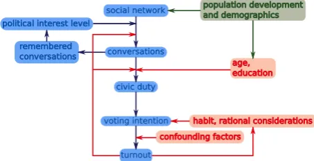
Model 1 is a complex agent-based computational model of voting, developed to incorporate the evidence suggested in the social science literature. This model describes the in-habitants of a neighbourhood or small city, and consists of a population of agents that occupy the sites of a square lattice, with sites corresponding to houses, workplaces, schools and other places of activity. The agents have a large number of characteristics (including age, ethnicity, interest in politics and “civic duty”) and are subjected to many processes (including ageing, moving house, finding jobs and having children). These processes modify some of the agents’ characteristics and allow them to make links to other agents, creating a social network. Agents also initiate (political) conversations over this social network, with a probability that depends on their political inter-est. In turn, the conversations they receive affect their political interest and allow civic duty to spread between agents. Agents’ civic duty (together with other elements) determines their propensity to vote in a series of peri-odic elections. Agents can leave the simulation by dying or emigrating and new agents are created via births and immigration. The details of the model can be found in ref-erences [15,16]. A schematic representation of the model is given in Figure1.
[image:3.595.313.540.97.213.2]In a recent work, Model 1 was distilled into the more compact Model 2. By neglecting some of the more com-plicated components of Model 1, Model 2 allowed us to investigate the effects of different mechanisms, and to ex-plore the parameter space in a more efficient way. A major simplification of Model 2 was ignoring all processes that form links between agents, setting instead a social network with appropriate characteristics. Other elements, such as
Fig. 1. Diagrammatic representation of the complex model. The main pathway is shown in blue, with additional factors in red, and general development of the agent population in green.
those regarding party preference and development of chil-dren, were also neglected. Model 2 achieved a large sim-plification (of the order of a factor 1000 in computational efficiency [17]) whilst maintaining good agreement with Model 1. A detailed description of the relatively complex Model 2 is given in AppendixA.
In this section we will push the model-analysis process forward. We will start by formulating Model 3, a simpler version of Model 2 that is more suitable for mathemati-cal analysis. Some of the simplifications we will make will involve formulating processes in a more standard form so that checking the output of these against those from Model 2 enables us to draw conclusions that are robust with respect to the implementation details.
In Model 2, social influence (the key mechanism in the model) is implemented using two main variables: inter-est level and number of conversations remembered. The interest level determines the propensity of an agent to ini-tiate conversations. In turn, the interest level of an agent is determined by the number of their received conversa-tions (together with their minimum interest level). Con-versations are forgotten with some probability every year. A further complication is that agents with zero interest level have different dynamics, until their number of ‘back-ground’ conversations remembered exceeds a given thresh-old (see AppendixA for details).
We will simplify Model 2 in three main ways to cre-ate Model 3. Firstly we will use the same dynamics for all interest levels (thus ignoring the difference in Model 2 for agents with interest level zero). In addition, we will use a single variable for the influence process, which we call the ‘interest state’, that increases with each received conversation and decreases appropriately, rather than one variable for interest level and a different one for conver-sations remembered. Moreover, we will uncouple the dy-namics of the interest state from that of voting. While in Model 2 agent’s voting behaviour affects their probability to initiate conversations (turnout-conversations feedback in Fig.1), this feedback will be neglected in Model 3.
2.1 Model 3 definition
The model consists of a population ofN agents. Agents enter and leave the model via immigration-emigration and birth-death. For simplicity we keep the population size constant, by matching each death event by a birth and every emigration by an immigration. Agents age through-out the simulation and their age determines their death probability. The ith agent is characterized by three dy-namic variables: (political) interest state,s(i); civic duty,
d(i); and voting habit,h(i). In addition, agents have two fixed characteristics: their ‘intrinsic interest’ state, m(i); and their level of education,ed(i). The interest state,s(i), is the primary dynamic variable in the model, controlling how often the agent initiates conversations, and depending on the number of received conversations. Civic duty,d(i), (spread through conversations) and voting habit,h(i), are binary variables that together determine the probability of an agent voting. Finally, the intrinsic interest state deter-mines the minimum value that the interest state variable may take for that agent, and the education modulates the probabilities of acquiring or losing civic duty.
We now describe the model dynamics.
(i) At each time step each agent initiatesBin(K, f(s(i), m(i))) conversations1, whereBin(N, p) is a binomial random variable for the number of successes fromN
trials, each with probabilitypof success.
(ii) For each successful conversation another agent,j, is picked at random (corresponding to a fully connected underlying network) and the receiving agent increases their interest state [s(j) →s(j) + 1]. Conversations can lead to the spread of civic duty in the following way. If a conversation takes place from an agent, i, with civic duty to an agent,j, without it, and agent
j’s interest state is larger than some threshold,s(j)≥
Td, then they gain civic duty with probability, ad, dependent on whether they voted in the last election. (iii) Each time step, after all conversations are completed, every agent has a probability [s(i)−m(i)]γ to de-crease their interest state by one. Thus in the absence of received conversations an agent’s interest state will decay to their intrinsic interest state over a time-scale of order 1/γ. In addition, agents lose civic duty with a probabilityldso that civic duty decays over a time-scale of order 1/ld (typicallyldγ).
(iv) Elections take place with periodicityτe. An agent will vote with probability (1-pc) if they have civic duty or voting habit, and will otherwise not vote. Here pc is the probability of not voting, despite having the tention to vote, due to “confounding factors”, for in-stance illness or having recently lost employment. An agent voting in three consecutive elections acquires voting habit, and loses this habit if they fail to vote in two consecutive elections.
1 If f(s(i), m(i)) > 1 then K + Bin(K, f(s(i), m(i))− f(s(i), m(i))) conversations are realised, wherex denotes the integer part of x. If K is not a natural number, then
[image:4.595.309.549.98.435.2]Bin(K, f(s(i), m(i))) +Bin(1,(K− K)f(s(i), m(i))).
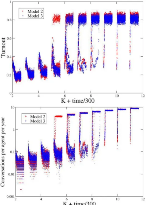
Fig. 2. Comparing the results for Model 2 (red circles) and Model 3 (blue pluses), in turnout (top figure) and number of conversations per year per agent (bottom, in log-scale to ap-preciate the low-conversations regime better). For each value of K (the influence rate), we plot 25 time series from 0 to 200 years. Herec= 3 and other parameter values are given in AppendixB.
We focus mainly on a fully connected underlying net-work to ease the analysis. By initially ignoring netnet-work effects we can better understand the main properties of the model. Network effects are considered at the end of Section 3.
2.2 Comparing Models 2 and 3
Page 4 of9 Eur. Phys. J. B(2016) 89: 159
turnout, for higher values of the influence rate. These two regimes are connected by a region of bistability, in which, for the same parameter values and initial conditions, some realisations converge to the ‘high-communication’ regime and some to the ‘low-communication’ one (which regime is achieved is a random outcome arising from the stochas-ticity of the process). We note that the results are similar when plotting the variables civic duty or voting habit.
We can also see from Figure 2 that results of Mod-els 3 and 2 show good agreement. The number of con-versations are very close for the two models. The main difference between the two models is that Model 3 gives a slightly smaller voter turnout. In the low-communication regime, this is primarily due to the simplifying assump-tion in Model 3 that individuals with zero interest state follow the same dynamics as those with higher interest states (which is not the case in Model 2). This leads to a smaller number of agents being susceptible to acquiring civic duty. In the high-communication regime, the differ-ence in turnout is mainly due to the assumption in Model 3 that the probability,pc, of an agent not voting in spite of having civic duty or voting habit, does not depend on age. In contrast in Model 2, the probability of an agent with civic duty or voting habit not voting is smaller for younger agents, so that agents in Model 2 are slightly more likely to build habit, leading to higher levels of voting (the aforementioned zero-interest effect is less important in this regime because almost no agent has interest state equal to zero). This explanation is confirmed by simulations which include these elements. Despite these small quantitative differences, Models 2 and 3 are qualitatively very similar.
3 Analysis
We would like to understand the origin of the low- and high-communication regimes and the bistability region, as well as the mechanisms required to observe these features. In order to do so, we will perform a general mathematical analysis of Model 3. Because the interest state dynamics is unaffected by the voting dynamics and yet interest and voting are closely correlated, we conclude that the interest state dynamics is the main driver of the system, and will focus our analysis on the interest state dynamics.
The process is a discrete-time analogue of the follow-ing system of continuous-time birth and death stochastic processes:
s(i)−→β s(i) + 1, s(i)−→δi s(i)−1, (1) with β ≡Kjf(s(j), m(j))/N and δi ≡[s(i)−m(i)]γ
(note that ifs(i) ≥ m(i) initially then δi is always pos-itive). We will analyse this continuous-time version for mathematical convenience.
In order to make analytical progress, we will assume thatβis time-independent. This is suggested by applying the central limit theorem, since β is the sum of N inde-pendent random variables divided byN (the central limit theorem does not strictly apply here, since thes(j) vari-ables are not independent, so the time-independence ofβ
is an assumption), and it is supported by numerical sim-ulations with large N. With the constantβ assumption, (1) implies that the variables s(i)−m(i) follow indepen-dent linear birth and death processes. At steady state, we have [18]:
s(i) =m(i) + Poissoni(λ), (2) whereλ≡β/γ, and Poissonj(λ) are Poisson random vari-ables with meanλ(independent for different values ofj). Under the constant λ assumption, inserting equa-tion (2) in the definition of λ, we obtain the following self-consistent equation:
λ=K
γ
j
f(m(j) + Poissonj(λ), m(j))
N . (3)
We can re-write the sum in (3) grouping agents with the same value of the minimum interest state,m:
N
j=1
f(m(j) + Poissonj(λ), m(j))
=
m
α∈Am
f(m+ Poissonα(λ), m), (4)
with Am equal to the set of indices of agents that have intrinsic state equal to m, Am = {j|m(j) = m}. As-suming thatAm is large for everym(i.e. there are many agents of each type) or, equivalently, disregarding fluctua-tions,α∈A
mf(m+ Poissonα(λ)) is just an average over a Poisson distribution with meanλ,
α∈Am
f(m+Poissonα(λ), m)≈ |Am|f(m+n, m);λ, (5)
where;λindicates an average over a Poisson distribution with mean λ, and |Am| denotes the number of elements in the set Am, |Am| = N P(m), with P(m) the fraction of agents with intrinsic interest state equal tom. Making this approximation, equation (3) leads to:
γ
Kλ=
m
P(m)f(m+n, m);λ ≡g(λ). (6)
Equation (6) displays the key elements in the system and it is the main result of this section. The social interac-tion appears through the funcinterac-tionf, the heterogeneity in the population via the average over the distribution ofm,
P(m), and the intrinsic stochasticity through the average over the Poisson distribution. The form of the equation de-pends on the mean-field-type of interaction (equivalently, fully connected social network) assumed. The equation shows how the interaction function, f, smoothed out by the heterogeneity and stochasticity, determines the num-ber and type of solutions asK/γis varied.
λ
0 10 20 30
g(
λ
)
[image:6.595.62.273.95.261.2]0 0.2 0.4 0.6 0.8 1
Fig. 3. Right-hand side of equation (6) (solid line) and left-hand side forK= 2 (dashed),K= 4 (dot-dashed) andK= 16 (dotted), for c = 3 and other parameter values as in Ap-pendixB. Between K= 2.8 andK= 10.4 the self-consistent equation (6) has three solutions.
We see that g(λ) displays an S-shape, starting at a small value forλ= 0, increasing for intermediate values of
λand saturating for larger values ofλ. The value ofg(λ) at
λ= 0 is related to the amount of conversations that take place even when social influence is absent (due to agents with large intrinsic interest), while the value of g(λ) for largeλcorresponds to the amount of conversations when all the agents have their maximum possible interest (due to large social influence). The position and sharpness of the increase depends on the form off as well as on the distribution ofm. The sharper f is, and the more homo-geneous the population, the sharper the increase ing(λ). We see that bistability is possible if g(λ) increases rela-tively sharply, which corresponds to a sharply increasingf
and a homogeneous population, and if limλ→∞g(λ)−g(0) is large (compared with g(0)), which corresponds to the case in which social influence has a strong impact on the overall conversation levels. This prediction is confirmed by numerical simulations of Model 3, as well as of Models 2 and 1, illustrating how the analysis of the simpler Model 3 can generate important insights into the behaviour of the more complex Model 1.
In Figure4the solutions of equation (6) are compared with numerical simulations, showing good agreement.
Figure 3 illustrates how for large values ofγ/K there is only one solution of equation (6). As γ/K decreases, the line (λ/K)γ becomes tangent to the right-hand side of (6), giving rise to two new solutions through a saddle-node bifurcation. Asγ/Kdecreases further, a new tangent condition is obtained, leading to the disappearance of two of the solutions through another saddle-node bifurcation. Imposing equation (6) together with the equality of the derivatives leads to:
λ= g(λ)
g(λ), (7)
K= γ
[image:6.595.311.547.98.268.2]g(λ). (8)
Fig. 4.Number of conversations per agent per year as a func-tion of parameter K, for c= 3 and year t= 200. Error bars correspond to two standard deviations. The red crosses corre-spond to runs in which the initial population had a low interest state while the blue diamonds correspond to runs with high initial interest. The simulations show a region of bistability betweenK= 4 andK= 9.
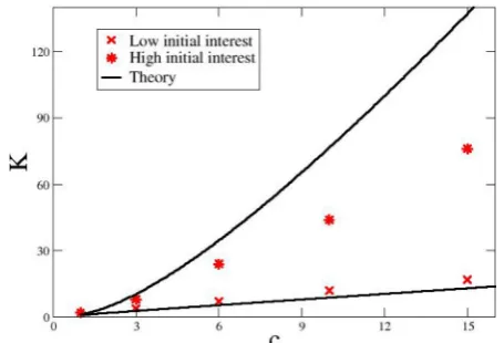
Fig. 5. Bistability region in the K-cplane. Bistability is ob-served for values ofK between the symbols. Theoretical pre-dictions are displayed as solid lines.
[image:6.595.314.542.361.516.2]Page 6 of9 Eur. Phys. J. B(2016) 89: 159
We see that, for reasonably large values of c, the bista-bility disappears much sooner in the simulations than in the theoretical predictions. This might be due to the fact that, while, in the deterministic limit, the solution corre-sponding to the low-communication regime still exists, its relative stability (and its basin of attraction) is low and the noise pushes the system to the ‘high-communication’ solution. This particularly simple bifurcation diagram is obtained when the function f used is taken to approxi-mate Model 2 (see Appendix B). For more general forms of the functionf a more complex bifurcation diagram is possible.
It is interesting to compare Model 3 with other mod-els of social influence. Threshold modmod-els of collective be-haviour [19,20] form probably the simplest class of models showing similar phenomenology. In these models, an agent participates in an activity if some proportion of the popu-lation (the agent’s threshold) also does so. Bistability can appear when the population is homogeneous (the thresh-old distribution is sharply peaked around a given value). Our model is similar to this class in that different agents require different amounts of social input in order to show the same level of activity (due to different intrinsic inter-ests,m). The random-field Ising model [21], which can also be used to model social phenomena [11,22,23], shows sim-ilar phenomenology, with multi-stability arising for small disorder and low noise. In this case, the local fields of the random-field Ising model would correspond to intrinsic in-terest of our model. The key ingredients of all these models are a heterogeneous population and a nonlinear influence function.
So far we have assumed a fully connected interaction network. The results can, however, change qualitatively when a different type of interaction network is used. The effects of the network in Model 3 are the same as those obtained for Model 2 [17]. The main result is that the bistability region can disappear, with the relevant vari-ables increasing in a smoother way, when the interaction network becomes sparse or strongly clustered. This effect is reminiscent of that found in random field Ising models in which sparser networks tend to require higher interaction strength for bistability to occur [23]. From the perspective of our analysis, adding a network leads to conversation in-puts that fluctuate more between agents. This results in an extra source of heterogeneity in the equation forλ(that in this case should be replaced byλ≡λi/N) that fur-ther smooths the interaction functionf, which results in a smaller region of parameter space in which bistability occurs. We note that since we expect real systems to be heterogeneous this result suggest that bistability may not be widespread in real-world systems.
4 Conclusions
In this paper we have demonstrated the power of a method of model reduction involving generating a chain of increasingly simpler models. Beginning from a com-plex model (Model 1), and a previously published re-duced model (Model 2), we have created a further rere-duced
model (Model 3) and shown that it agrees quantitatively and qualitatively with Model 2. Since the relationship of Model 2 to Model 1 has been previously investigated, we thus have a clear link between results derived and un-derstood in Model 3 to equivalent effects found in the original complex model, which in turn explicitly models mechanisms believed to be important in real world voting processes.
We have described some advantages of this approach in the Introduction, but one of the most compelling is that it combines the best of two worlds: the simplicity appreciated by those trained in the physical sciences, but having an input from the many effects included in com-plex models. A central point is that, although the mod-els constructed through this procedure are ‘simple’, in the sense that they have far fewer parameters than the models they are derived from and are more amenable to analysis, they will typically have features that would not have been guessed at if one started from simple models and then added further complexity. This is the strength of the ap-proach: Model 1 contains within it a large amount of social science data and expertise, and a diluted form of this is retained in Model 3.
A direct translation of the methods used in physics would be to start with a minimal model, progressively introducing new structure and at every stage comparing the new model with data. We believe that the process we have described here is more directly suited to the social sciences, with its relative paucity of data. However the conventional physical sciences approach can still have a role after the various stages of models have been created. One could also attempt to go from Model n to Model (n−1), and in this way explore a wide range of possible models by going up and down the various stages. In this way one should be able to gain a fuller appreciation of the role that various extra structures have in giving a more complete description of the system.
To demonstrate the utility of creating a model that is amenable to mathematical analysis we have used Model 3 to investigate the origins of the bistability seen in Model 2, and the existence of high and low turnout regimes found in both Models 2 and 1. This investigation allowed us to un-derstand the mechanisms required for bistability to exist, and provided an explanation for the observed dependence on the homogeneity of the population and the structure of the social network when one is used. This was a specific illustration of the use of this method in models of voter turnout, but we believe that the present approach of using a chain of increasingly simple models can be fruitful for the analysis of a wide variety of complex systems.
Author contribution statement
AJM and BE designed the research, LFL and LD per-formed the research, LFL, LD, AJM and BE wrote the paper.
Appendix A: Description of Model 2
The description of Model 2 can be found in reference [17]; we give it here for completeness.
Each agent (with indexi= 1, . . . , N) has the following list of characteristics, some of which can change over time:
binary variables:civic duty (cd(i)), turnout (in last election, v(i)), voting habit (h(i)), post-18 education (ed(i))
integer variables: (political) interest level (l(i)), minimum interest level (m(i)), age (in years, a(i)), number of (political) conversations remembered (c(i)).
The main parameters of the model are:
Influence rateK, which scales the number of (political) conversations per year.
Probabilities of initiating a conversationpc(l, v). Probabilities of gaining and losing civic dutypacd(e, v) andplcd(e, v, a), respectively.
Thresholds on the number of conversations needed to increase the interest levelTα.
Probability of forgetting a conversationpf(l). Death probabilitypd(a).
Emigration probabilitype.
Probability of not voting due to confounding factors
pc(a).
A.1 Initialisation procedures
Agents are initialised using data derived from the British Household Panel Study (BPS) [24]. The same procedure initialises immigrants into the model, using the subset of the BHPS corresponding to survey responses from immi-grants. This procedure sets the civic duty, turnout, vot-ing habit, post-18 education, interest level and minimum interest level, with some of these characteristics being in-ferred using proxies for the required information. Agents initially do not remember any conversations, and have an age drawn from a uniform distribution between 18 and 70 (to initialise the model) and between 18 and 48 (for later immigrants into the model). Agents born into the simula-tion have age 18 (they are only taken into account in the model when they are adults), and education with proba-bility 0.3. Their interest level and minimum interest level is equal to their education, and they are assumed have no civic duty, voting habit or conversations remembered and not to have voted in the last election.
A.2 Main loop
The following processes happen in a loop until the required time-point is reached. All rates are given in Table A.1 below.
Each year:
Each month:
Carrying out conversations: For each agent, this section is run K/12times plus one time extra with probability K/12− K/12.
The agent has the chance to initiate three con-versations, with probabilitiespc(l(i), v(i)) each with a random other agent.
Agents (withl(i)>0) receiving a conversation (from an agent with civic duty), acquire civic duty with probabilitypacd(ed(i), v(i)).
Updating interest levels:
Ifl(i) = 0 andc(i)> T0 then setl(i) = 1 and
m(i) = 1.
Else, ifc(i)> Th then setl(i) =m(i) + 2. Else, ifc(i)> Tl then setl(i) =m(i) + 1.
Updating civic duty:Agents lose civic duty with probability,plcd(ed(i), v(i)), dependent on their age and education.
Forgetting conversations: Agents forget conversa-tions that happened more than one year ago, with probability, pf(l(i)), per conversation, dependent on the agent’s interest level.
Birth/death: Each agent dies with a probability,
pd(a(i)), dependent on their age, and is replaced by a new agent by the ‘birth’ process (described in Sect.A.1).
Immigration/emigration: Each agent emigrates with a probability pe = 0.015 and is replaced by a new agent by the ‘immigration’ process (described in Sect.A.1).
Ageing:Agents age by one year.
Every 5 years there is an election:
Agents with civic duty or voting habit vote unless ‘con-founded’ (due to illness or other factors) with proba-bilitypc(a(i)), dependent on their age.
Agents gain voting habit if they vote in 3 consecutive elections.
Agents lose voting habit if they do not vote in 2 con-secutive elections.
Here xdenotes the integer part ofx, that is, the largest integer no greater thanx.
Appendix B: Parameters for Model 3
In the main text, Model 3 has been defined in rather general terms. In order to correspond to Model 2 as de-scribed in AppendixA, it is necessary to make the follow-ing identifications:
The social interaction function f has to take the fol-lowing piece-wise constant form:
f(s, m) =
⎧ ⎪ ⎪ ⎪ ⎪ ⎪ ⎪ ⎪ ⎪ ⎪ ⎨ ⎪ ⎪ ⎪ ⎪ ⎪ ⎪ ⎪ ⎪ ⎪ ⎩
0, ifs <2c.
0.322≡f1, if 2c≤s <3c.
0.794≡f2, if 3c≤s <4c.
0.794≡f2, ifs≥4c andm <2c.
1.397≡f3, ifs≥4c andm≥2c.
(B.1)
Page 8 of9 Eur. Phys. J. B(2016) 89: 159
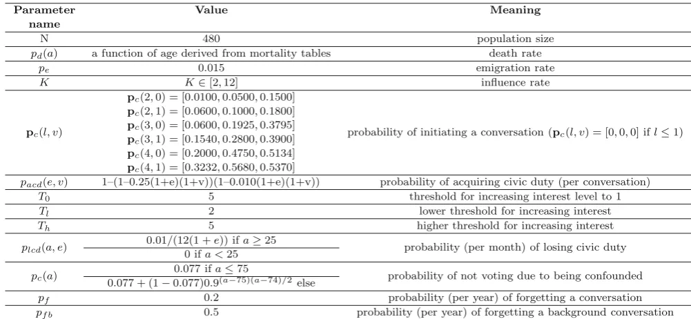
Table A.1. Parameter values for Model 2.
Parameter Value Meaning
name
N 480 population size
pd(a) a function of age derived from mortality tables death rate
pe 0.015 emigration rate
K K∈[2,12] influence rate
pc(l, v)
pc(2,0) = [0.0100,0.0500,0.1500]
probability of initiating a conversation (pc(l, v) = [0,0,0] ifl≤1)
pc(2,1) = [0.0600,0.1000,0.1800]
pc(3,0) = [0.0600,0.1925,0.3795]
pc(3,1) = [0.1540,0.2800,0.3900]
pc(4,0) = [0.2000,0.4750,0.5134]
pc(4,1) = [0.3232,0.5680,0.5370]
pacd(e, v) 1–(1–0.25(1+e)(1+v))(1–0.010(1+e)(1+v)) probability of acquiring civic duty (per conversation)
T0 5 threshold for increasing interest level to 1
Tl 2 lower threshold for increasing interest
Th 5 higher threshold for increasing interest
plcd(a, e)
0.01/(12(1 +e)) ifa≥25
probability (per month) of losing civic duty 0 ifa <25
pc(a) 0.077 ifa≤75 probability of not voting due to being confounded
0.077 + (1−0.077)0.9(a−75)(a−74)/2else
pf 0.2 probability (per year) of forgetting a conversation
pf b 0.5 probability (per year) of forgetting a background conversation
affected by whether or not the agent voted in the previous election. This link is broken in Model 3. In order to have comparable values forf, we choose the ones corresponding to Model 2, assuming that the agent voted with a proba-bility of 0.86. This is approximately equal to the propor-tion of agents voting in the high-communicapropor-tion regime (we expect it to work as well on the low-communication regime because the few agents that initiate conversations in that regime are also likely to have voted).
The probability of acquiring and losing civic duty is given by:
ad=
⎧ ⎪ ⎪ ⎨ ⎪ ⎪ ⎩
0.258, ifv(i) =ed(i) = 0.
0.51, ifv(i) = 1, ed(i) = 0 orv(i) = 0, ed(i) = 1.
1, ifed(i) =v(i) = 1.
(B.2)
ld=
0.000417, ifed(i) = 0.
0.00083, else.
(B.3)
Other parameter values areγ= 0.0167 month−1,Td=c,
pc = 0.139,τe= 5 years. The total number of individuals isN = 500. Alsoc= 3 unless otherwise stated.
Individuals born in the simulation are initiated with 18 years of age (we do not explicitly include children), with:
ed(i) =B(0.34), m(i) =c·ed(i), v(i) =h(i) =d(i) = 0. The characteristics of immigrants are set based on statistics derived from the British Household Panel Study [24], as follows:
m(i) = 3c,2c, c,0, with probabilities 0.02, 0.06, 0.21, 0.71, respectively.
If m(i) = 3c, thens(i) = 4c,ed(i) =d(i) = 1, v(i) =
B(0.9),h(i) =B(0.29).
Ifm(i) = 2c, thens(i) = 3c+B(0.32),ed(i) =B(0.68),
d(i) =B(0.43),v(i) =B(0.70),h(i) =B(0.13). If m(i) =c, thens(i) =c,ed(i) = 1, d(i) =B(0.21),
v(i) = 0.72,h(i) =B(0.13).
Ifm(i) = 0, thens(i) = c, ed(i) = 0, d(i) =B(0.21),
v(i) = 0.72,h(i) =B(0.13).
In addition, if h(i) = v(i) = 1, with probability 0.9 it is assumed that the agent voted in the election previous to the latest one (this is relevant for the dynamics of vot-ing habit). Here B(x) denotes a Bernoulli random vari-able with mean x, that is B(x) = 1 with probability x,
B(x) = 0 else. These parameter values are taken directly from Model 2, with no data fitting involved.
With the form off(s, m) given in (B.1), equation (6) becomes:
γ
Kλ=P(0)f2+P(1)f2+P(2)f3+P(3)f3
−Γ(c, λ)
Γ(c) [P(1)f1+P(2)(f2−f1)+P(3)(f3−f2)]
−Γ(2c, λ)
Γ(2c) [P(0)f1+P(1)(f2−f3)+P(2)(f3−f2)]
−Γ(3c, λ)
Γ(3c) P(0)(f2−f1), (B.4)
where Γ(a) = Γ(a,0) is the Gamma function, and
Γ(a, x) ≡ x∞ta−1e−tdt is the incomplete Gamma func-tion. Since Γ(a, x)/Γ(a) decreases monotonically withx, withΓ(a,0)/Γ(a) = 1, Γ(a,∞)/Γ(a) = 0, Γ(a, a)/Γ(a)≈ 1/2 (last approximate equality being valid for large a), we see that the right-hand side of (B.4) changes from
of (B.4) typically displays an S-shape which can lead to several solutions for λin a range of parameter values, as illustrated in Figure3in the main text.
Forλc, equation (B.4) simplifies to:
γ
KλP(2)f1+P(3)f2⇒γλK[P(2)f1+P(3)f2],
(B.5) while forλc, equation (B.4) leads to:
γ
Kλ[P(0) +P(1)]f2+ [P(2) +P(3)]f3
⇒γλK{[P(0) +P(1)]f2+ [P(2) +P(3)]f3}. (B.6)
We see that both the solution with smallλ and the one with large λ, increase linearly with K. This simple ap-proximation breaks down for intermediate values ofλ(of the order ofc), but it can be rather accurate, as evidenced by the approximately straight character of the theoretical lines in Figure4of the main text.
References
1. The Social Logic of Politics, edited by A.S. Zuckerman (Temple University Press, Philadelphia, 2005)
2. M. Rolfe, Voter Turnout: A Social Theory of Political Participation (Cambridge University Press, New York, 2012)
3. B. Sinclair, The Social Citizen: Peers Networks and Political Behavior (University of Chicago Press, Chicago, 2012)
4. D.W. Nickerson, Am. Polit. Sci. Rev.102, 49 (2008) 5. R.M. Bond, C.J. Fariss, J.J. Jones, A.D.I. Kramer, C.
Marlow, J.E. Settle, J.H. Fowler, Nature489, 295 (2012) 6. N. Goldenfeld, L.P. Kandanoff, Science284, 87 (1999) 7. A.T. Bernardes, D. Stauffer, J. Kert´esz, Eur. Phys. J. B
25, 123 (2002)
8. M. Gonzalez, A. Sousa, H. Herrmann, Int. J. Mod. Phys. C15, 45 (2004)
9. C. Borghesi, J.-P. Bouchaud, Eur. Phys. J. B 75, 395 (2010)
10. C. Borghesi, J.-C. Raynal, J.-P. Bouchaud, PloS One 7, e36289 (2012)
11. S. Galam, S. Moscovici, Eur. J. Soc. Psychol.21, 49 (1991) 12. J.H. Fowler, inThe Social Logic of Politics, edited by A.S. Zuckerman (Temple University Press, Philadelphia, 2005), pp. 296–287
13. C. Fosco, A. Laruelle, A. S´anchez, Adv. Complex Syst.14, 31 (2011)
14. J. Fern´andez-Gracia, K. Suchecki, J.J. Ramasco, M. San Miguel, V.M. Egu´ıluz, Phys. Rev. Lett. 112, 158701 (2014)
15. B. Edmonds, L. Lessard-Phillips, E. Fieldhouse, A complex model of voter turnout (version 1), CoMSES Computa-tional Model Library,https://www.openabm.org/model/ 4368/version/1 (2014)
16. T. Loughran, L. Lessard-Phillips, E. Fieldhouse, B. Edmonds, The voter model – a long description, SCID project document, https://scidproject. files.wordpress.com/2015/05/the-voter-model-description-final-draft.docx (2015)
17. L.F. Lafuerza, L. Dyson, B. Edmonds, A.J. McKane, arXiv:1604.00903 (2016)
18. N.G. Van Kampen, inStochastic Processes in Physics and Chemistry (Elsevier, Amsterdam, 2007), p. 145
19. M. Granovetter, Am. J. Sociol. 83, 1420 (1978) 20. D.A. Siegel, Am. J. Polit. Sci.53, 122 (2009)
21. J.P. Sethna, K. Dahmen, S. Kartha, J.A. Krumhansl, B.W. Roberts, J.D.Shore, Phys. Rev. Lett.70, 3347 (1993) 22. Q. Michard, J.-P. Bouchaud, Eur. J. Soc. Psychol.47, 151
(2005)
23. J.-P. Bouchaud, J. Stat. Phys.151, 567 (2013)
24. British household panel study (BHPS), https://www. iser.essex.ac.uk/bhps