Gap junctions, dendrites and resonances : a recipe for tuning network dynamics

http://wrap.warwick.ac.uk

Original citation:

Timofeeva, Yulia, Coombes, Stephen and Michieletto, Davide. (2013) Gap junctions,

dendrites and resonances : a recipe for tuning network dynamics. The Journal of

Mathematical Neuroscience, Volume 3 (Number 1). Article number 15. ISSN 2190-8567

Permanent WRAP url:

http://wrap.warwick.ac.uk/58464

Copyright and reuse:

The Warwick Research Archive Portal (WRAP) makes this work of researchers of the

University of Warwick available open access under the following conditions.

This article is made available under the Creative Commons Attribution 2.0 Generic (CC

BY 2.0) license and may be reused according to the conditions of the license. For more

details see:

http://creativecommons.org/licenses/by/2.0/

A note on versions:

The version presented in WRAP is the published version, or, version of record, and may

be cited as it appears here.

DOI10.1186/2190-8567-3-15

R E S E A R C H Open Access

Gap Junctions, Dendrites and Resonances:

A Recipe for Tuning Network Dynamics

Yulia Timofeeva·Stephen Coombes· Davide Michieletto

Received: 20 December 2012 / Accepted: 12 April 2013 / Published online: 14 August 2013

© 2013 Y. Timofeeva et al.; licensee Springer. This is an Open Access article distributed under the terms of the Creative Commons Attribution License (http://creativecommons.org/licenses/by/2.0), which permits unrestricted use, distribution, and reproduction in any medium, provided the original work is properly cited.

Abstract Gap junctions, also referred to as electrical synapses, are expressed along the entire central nervous system and are important in mediating various brain rhythms in both normal and pathological states. These connections can form between the dendritic trees of individual cells. Many dendrites express membrane channels that confer on them a form of sub-threshold resonant dynamics. To obtain insight into the modulatory role of gap junctions in tuning networks of resonant dendritic trees, we generalise the “sum-over-trips” formalism for calculating the response function of a single branching dendrite to a gap junctionally coupled network. Each cell in the network is modelled by a soma connected to an arbitrary structure of dendrites with resonant membrane. The network is treated as a single extended tree structure with dendro-dendritic gap junction coupling. We present the generalised “sum-over-trips” rules for constructing the network response function in terms of a set of coefficients defined at special branching, somatic and gap-junctional nodes. Applying this frame-work to a two-cell netframe-work, we construct compact closed form solutions for the net-work response function in the Laplace (frequency) domain and study how a preferred frequency in each soma depends on the location and strength of the gap junction.

Keywords Dendrites·Gap junctions·Resonant membrane·Sum-over-trips· Network dynamics

Y. Timofeeva (

Department of Computer Science and Centre for Complexity Science, University of Warwick, Coventry, CV4 7AL, UK

e-mail:[email protected]

S. Coombes

School of Mathematical Sciences, University of Nottingham, Nottingham, NG7 2RD, UK e-mail:[email protected]

D. Michieletto

1 Introduction

It has been known since the end of the nineteenth century and mainly from the work of Ramón y Cajal [1] that neuronal cells have a distinctive structure, which is dif-ferent to that of any other cell type. The most extended parts of many neurons are dendrites. Their complex branching formations receive and integrate thousands of in-puts from other cells in a network, via both chemical and electrical synapses. The voltage-dependent properties of dendrites can be uncovered with the use of sharp mi-cropipette electrodes and it has long been recognised that modelling is essential for the interpretation of intracellular recordings. In the late 1950s, the theoretical work of Wilfrid Rall on cable theory provided a significant insight into the role of dendrites in processing synaptic inputs (see the book of Segev et al. [2] for a historical per-spective on Rall’s work). Recent experimental and theoretical studies at a single cell level reinforce the fact that dendritic morphology and membrane properties play an important role in dendritic integration and firing patterns [3–5]. Coupling neuronal cells in a network adds an extra level of complexity to the generation of dynamic patterns. Electrical synapses, also known as gap junctions, are known to be impor-tant in mediating various brain rhythms in both normal [6,7] and pathological [8–10] states. They are mechanical and electrically conductive links between adjacent nerve cells that are formed at fine gaps between the pre- and post-synaptic cells and per-mit direct electrical connections between them. Each gap junction contains numerous connexon hemi-channels, which cross the membranes of both cells. With a lumen di-ameter of about 1.2 to 2.0 nm, the pore of a gap junction channel is wide enough to allow ions and even medium-sized signalling molecules to flow from one cell to the next thereby connecting the two cells’ cytoplasm. Being first discovered at the giant motor synapses of the crayfish in the late 1950s, gap junctions are now known to be expressed in the majority of cell types in the brain [11]. Without the need for recep-tors to recognise chemical messengers, gap junctions are much faster than chemical synapses at relaying signals.

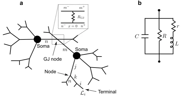
Fig. 1 aA network of two cells connected by a gap junction (GJ).bAn ‘LRC’ circuit modelling the resonant cell membrane

“sum-over-trips” method is built on the path integral formulation and calculates the Green’s function on an arbitrary dendritic geometry as a convergent infinite series solution.

In Sect.2, we introduce the network model for gap junction coupled neurons. Each neuron in the network comprises of a soma and a dendritic tree. Cellular mem-brane dynamics are modelled by an ‘LRC’ (resonant) circuit. In Sect.3, we focus on an example of two unbranched dendritic cells, with no distinguished somatic node, with identical and heterogeneous sets of parameters and give the closed form solu-tion for network response with a single gap juncsolu-tion. The complete “sum-over-trips” rules for the more general case of an arbitrary network geometry are also presented. In Sect.4, we apply the formalism to a more realistic case of two coupled neurons, each with a soma and a branching structure. We introduce a method of ‘words’ to construct compact solutions for the Green’s function of this network and study how a preferred frequency in each soma depends on the location and strength of the gap junction. Finally, in Sect.5, we consider possible extensions of the work in this pa-per.

2 The Model

subthreshold synaptic activity [19]. From a mathematical perspective, Mauro et al. [20] have shown that a linearisation of channel kinetics (for currents such as Ih), about rest, may adequately describe the observed resonant dynamics. The resulting linear system has a membrane impedance that displays resonant-like behaviour due to the additional presence of inductances (which are determined by the choice of channel model). This circuit is described by the specific membrane capacitanceC, the resistance across a unit area of passive membraneRand an inductanceLin series with a resistancer. The transmembrane voltageVi(x, t)on an individual branchiof each cell is then governed by the following set of equations:

∂Vi

∂t =Di ∂2_V

i

∂x2 − Vi

τi −

1

Ci[Ii−Iinj,i], (1)

Li∂I_∂ti = −riIi+Vi, 0≤x≤Li, t≥0. (2)

The constantsDi andτi can be found in terms of the electrical parameters of the cell membrane as Di =ai/(4Ra,iCi)and τi =CiRi, where ai is a diameter and

Ra,i is the specific cytoplasmic resistivity of branchi. The termIinj,i(x, t)models an external current applied to this branch. The dendritic structure of each cell is attached to an equipotential soma of the diameteras modelled by the ‘LRC’ circuit with the

parametersCs,Rs,Lsandrs. Moreover, individual branches of different cells can be connected by gap junctions with a coupling parameterRGJ.

Equations (1)–(2) for each dendritic segment must be accompanied with addi-tional equations describing the dynamics of voltage at two ends of a segment. If the proximal (x=0) or distal (x=Li) end of a branch is a branching node point the con-tinuity of the potential across a node and Kirchoff’s law of conservation of current are imposed. For example, boundary conditions for a node indicated in Fig.1a take the form:

Vj(Lj, t)=Vn(0, t)=Vk(0, t), (3)

1

ra,j

∂Vj

∂x

_x

=Lj =

1

ra,n

∂Vn

∂x

_x

=0

+_r1

a,k

∂Vk

∂x

_x

=0

, (4)

wherera,j=4Ra,j/(πa_j2)is the axial resistance on branchj. If a branch terminates atx=Li we either have a no-flux (a closed-end) boundary condition

∂Vi

∂x

_x

=Li=0, (5)

or a zero value (an open-end) boundary condition

Vi(Li, t)=0. (6)

conditions on the proximal ends of branches connected to the soma:

Vs(t)=Vj(0, t), (7)

CsdVs

dt = −

Vs Rs + j 1 ra,j ∂Vj ∂x _x =0

−Is, (8)

Ls

dIs

dt = −rsIs+Vs, (9)

where the sum in Eq. (8) is over all branches connected to the soma. If the branches of two cells are coupled by a gap junction, the location of this coupling can be treated as a special node point on an extended branching structure. This gap-junctional (GJ) node requires the following set of boundary conditions (given here with an assump-tion that it is placed atx=0):

V_m−(0, t)=Vm+(0, t), Vn−(0, t)=Vn+(0, t), (10)

and 1 ra,m _∂V m− ∂x _x =0

+∂V_∂xm+

x=0

=gGJVm−(0, t)−Vn−(0, t), (11)

1 ra,n _∂V n− ∂x _x =0

+∂V_∂xn+

x=0

=gGJVn−(0, t)−Vm−(0, t), (12)

wheregGJ=1/RGJis the conductance of the gap junction andm−andm+(n−and

n+_{) are two segments of branchm (branchn) connected at the gap junction (see} Fig.1a). The expressions in (10) reflect continuity of the potential across individual branchesmandn, and Eqs. (11)–(12) enforce conservation of current.

A whole network model can be viewed as an extended tree structure with each individual node belonging to one of the following categories: a terminal, a regular branching node, a somatic node or the GJ node. The voltage dynamics along the net-work structure are described by linear equations and, therefore, the model’s behaviour can be studied by constructing the network response function known as the Green’s function,Gij(x, y, t). This function describes the voltage response at the locationx on branchiin response to a delta-Dirac pulse applied to the locationy on branch

j at time t=0 (branchesi andj can belong either to the same cell or to the two different cells). Knowing the Green’s function for the whole structure, it is easy to compute the voltage dynamics along the whole network for any form of an external inputIinj,j(x, t)applied to branchj as

Vi(x, t)=

k

_Lk

0

dyGik(x, y, t)Vk(y,0)

+ t 0 ds _Lj 0

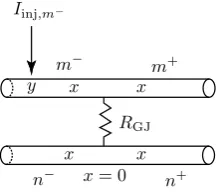
Fig. 2 A network of two identical cells, each consists of an infinite dendritic cable, coupled by a gap junction

whereVk(x,0)describes the initial conditions on branchk and the sum is over all branches of the tree. Multiple external stimuli can be tackled by simply adding new terms with additional inputsIinj,j(x, t)to Eq. (13).

3 The Green’s Function on a Network

Earlier work of Coombes et al. [17] demonstrated that the Green’s function for a sin-gle cell with resonant membrane can be constructed by generalising the “sum-over-trips” framework of Abbott et al. [15,16] for passive dendrites. Here, we demonstrate how this framework can be extended to a network level starting with the simple case of two identical cells.

3.1 Two Simplified Identical Cells

We consider the case of two identical cells coupled by a gap junction. Each cell consists of a single resonant dendrite of infinite length (see Fig. 2). A gap junc-tion controlled by the parameterRGJand located atx=0 divides two dendrites into

four semi-infinite segments:m−,m+,n−, andn+. We assume that an external input

Iinj,m−(x, t)=δ(x−y)δ(t)is applied to segmentm−. The Green’s function on each

segment must satisfy the set of Eqs. (1)–(2) with the boundary conditions at the gap junction given by Eqs. (10)–(12). Introducing the Laplace transform with spectral parameterω

L f (t)=f (ω) =

_∞

0

e−ωtf (t)dt,

and assuming zero initial data, we can solve this model in the frequency domain:

Gm−(x, y, ω)= 1

C

e−γ (ω)|x−y|

2Dγ (ω) −pGJ(ω)

e−γ (ω)|x+y| 2Dγ (ω)

, (14)

Gm+(x, y, ω)= 1

C

1−pGJ(ω)

e−γ (ω)|x+y| 2Dγ (ω)

, (15)

G_n−(x, y, ω)=Gn+(x, y, ω)= 1

C

pGJ(ω)

e−γ (ω)|x+y| 2Dγ (ω)

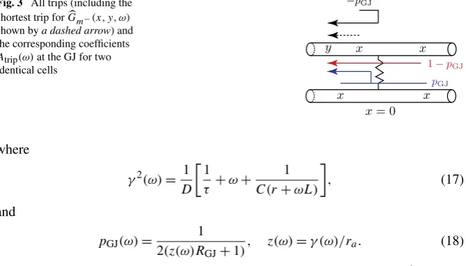
Fig. 3 All trips (including the shortest trip forGm−(x, y, ω)

shown bya dashed arrow) and the corresponding coefficients

Atrip(ω)at the GJ for two

identical cells

where

γ2_(ω)= 1 D

1

τ +ω+

1

C(r+ωL)

, (17)

and

pGJ(ω)= 1 2(z(ω)RGJ+1)

, z(ω)=γ (ω)/ra. (18)

Solutions (14)–(16) are obtained using the “sum-over-trips” method whereG(x, y, ω) on each segment can be found as_tripsAtrip(ω)G∞(Ltrip, ω), and

G_∞(x, ω)=e−γ (ω)|x|

2Dγ (ω) (19)

is the Laplace transform of the Green’s functionG_∞(x, t) for an infinite resonant cable.Ltripis the length of a path that starts at pointx on one of the segments and

ends at pointyon segmentm−. The trip coefficientsAtrip(ω)which ensure that the boundary conditions at the gap junction hold are chosen according to the following rules (see Fig.3):

• Atrip(ω)= −pGJ(ω) if the trip reflects along on the gap junction back onto the same dendrite.

• Atrip(ω)=1−pGJ(ω)if the trip passes through the gap junction along the same dendrite.

• Atrip(ω)=pGJ(ω) if the trip passes through the gap junction from one cell to

another cell.

Performing the numerical inverse Laplace transform (L−1_{) of Eqs. (14)–(16), we}

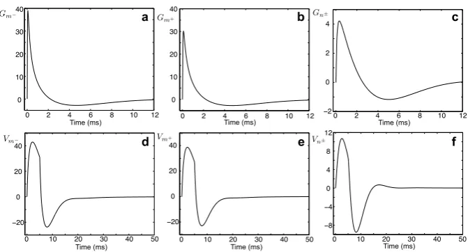
obtain the Green’s function in the time domain for each segment. These Green’s func-tions are plotted in Figs.4a–c. For any arbitrary form of external inputIinj,m−(x, t)=

δ(x−y)I (t), the voltage response on each segment can be found by taking a con-volution of the corresponding Green’s function with this stimulus. Using the Laplace representation of the Green’s function on each segment given by Eqs. (14)–(16) this can be computed as

Vk(x, t)=L−1 Gk(x, y, ω)I (ω), k∈m−, m+, n−, n+, (20)

Fig. 4 a–cThe Green’s functionsGm−(x, y, t),Gm+(x, y, t), andGn±(x, y, t)for a model in Fig.2

whenx=10 μm andy=100 μm. Parameters:a=2 μm,D=50000 μm2/ms,τ=2 ms,C=1 μF/cm2,

Ra=100cm,r=100cm2,L=5 H cm2,RGJ=100 M.d–fVoltage profiles on each segment in

response to a rectangular pulse of strengthη0=2 nA and durationτR=5 ms applied to segmentm−. Note that differenty-axislimits are used incandf

A response of the network model is characterised by the Green’s function and can be studied by introducing a power functionPk(x, y, ω)defined asPk(x, y, ω)=

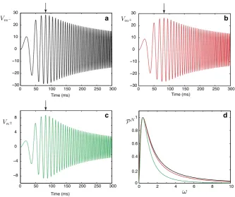
|Gk(x, y, ω)|2. Resonant dynamics of the model for a given pair of locations(x, y) are directly linked with a valueΩ0at which the functionPk(x, y, ω)has its max-imum. In Figs.5a–c, we plot the voltage profiles on each segment in response to a chirp stimulus Ichirp(t)=Achirpsin(ωchirpt2). These figures clearly demonstrate

resonant behaviour of the system maximising the voltage responses for particu-lar frequencies. In Fig.5d, we plot the normalised power functionsP_kN(x, y, ω)=

Pk(x, y, ω)/maxω[Pk(x, y, ω)]at the same locations. These power functions have their maximum at the valueΩ0=0.4271, the same for each segment and, therefore, the resonances (indicated by arrows) in Figs.5a–c occur at the same time. We can also notice that the functionP_nN_±(x, y, ω)decays to zero more rapidly than the func-tionsP_mN−(x, y, ω)andPmN+(x, y, ω). This explains the rapid reduction of voltage amplitude straight after the resonance in Fig.5c.

Typical values of a unitary gap junction conductance are 10–550 pS [11] giving

gGJ=10–5500 pS (orRGJ=180–105M) for 1–10 gap junction channels per

elec-trical connection, although these estimates may be conservative and conductances from a larger range could be considered, as for examplegGJ=10–240000 pS

Fig. 5 a–cVoltage profiles on each segment atx=10 μm in response to a stimulusIchirp(t)applied at

y₌100 μm on segmentm−. Cells’ parameters as in Fig.4,ωchirp=0.003,Achirp=1 nA.dNormalised

power functionsP_mN₋(x, y, ω)(black curve),P_mN₊(x, y, ω)(red curve),P_nN_±(x, y, ω)(green curve)

Fig. 6 a–cThe Green’s functionsGm−(x, y, t),Gm+(x, y, t), andGn±(x, y, t)for a model in Fig.2

whenx=10 μm andy=100 μm. Parameters:a=2 μm,D=50000 μm2/ms,τ=2 ms,C=1 μF/cm2,

Ra=100 cm, r=100 cm2, L=5 H cm2, RGJ =100 M (black curves, as in Figs.4a–c),

R_GJ=1 M(red curves),RGJ=1000 M(green curves). Note that differenty-axislimits are used

inc

identical cells, the change of the resistance of the gap junction does not affect the resonant frequencyΩ0, which is the same for each segment.

Fig. 7 a–cThe Green’s functionsG_m−(x, y, t),G_m+(x, y, t), andG_n±(x, y, t)for a model in Fig.2

with passive membrane whenx=10 μm andy=100 μm. Parameters:a=2 μm,D=50000 μm2/ms,

τ₌2 ms,C=1 μF/cm2,Ra=100cm,RGJ=100 M.d–fVoltage profiles on each segment in

response to a rectangular pulse of strengthη0=2 nA and durationτR=5 ms applied to segmentm−.

Note that differenty-axislimits are used incandf

possible to make extra progress and find analytical forms of the solutions in the time domain (see AppendixA). In Figs.7a–c, we plot the Green’s functions for the model in Fig.2 with passive (instead of resonant) membrane. Voltage responses on each segment in response to a rectangular pulse are shown in Figs.7d–f.

3.2 Two Simplified Non-identical Cells

Here, we consider a model in Fig. 2 with the assumption that the cells are non-identical. Then using the Laplace transform and solving the model (with zero initial data) in the frequency domain, we obtain

Gm−(x, y, ω)= 1

Cm

e−γm(ω)|x−y|

2Dmγm(ω) −pGJ,n(ω)

e−γm(ω)|x+y|

2Dmγm(ω)

, (21)

G_m+(x, y, ω)= 1

Cm

1−pGJ,n(ω)

e−γm(ω)|x+y|

2Dmγm(ω)

, (22)

G_n−(x, y, ω)=Gn+(x, y, ω)= 1

Cm

pGJ,m(ω)

e−|γn(ω)x+γm(ω)y|

2Dmγm(ω)

, (23)

where the parametersγm(ω)andγn(ω)are defined in terms of cells’ individual prop-erties as

γ2

m(ω)=_D1 m

1

τm+ω+

1

Cm(rm+ωLm)

, (24)

γ2

n(ω)=_D1 n

1

τn +ω+

1

Cn(rn+ωLn)

Fig. 8 All trips (including the shortest trip forGm−(x, y, ω)

shown bya dashed arrow) and the corresponding coefficients

Atrip(ω)at the GJ for two

non-identical cells

Solutions (21)–(23) show that the trip coefficientsAtrip(ω)depend on eitherpGJ,m(ω)

orpGJ,n(ω)(see Fig.8), which have the forms

pGJ,m(ω)=

zm(ω)

zm(ω)+zn(ω)+2RGJzm(ω)zn(ω), zm(ω)=γm(ω)/ra,m, (26)

pGJ,n(ω)=_z zn(ω)

m(ω)+zn(ω)+2RGJzm(ω)zn(ω)

, zn(ω)=γn(ω)/ra,n. (27)

In Figs.9a–c, we demonstrate how individual variations in cell parameters affect the voltage response in the system. For each set of the parameters, we plot the Green’s functionsGm−(x, y, t),Gm+(x, y, t), andGn±(x, y, t)obtained by taking the numer-ical inverse Laplace transform of (21)–(23). Black curves show the profiles for two identical cells. Dashed red curves are the Green’s functions for a case whenLn is changed from 5 H cm2to 25 H cm2. This change affects the response in Celln, but not in Cellm. Blue curves are plotted for a case whenLmis changed from 5 H cm2 to 1 H cm2. It has noticeable effect on both cells. Finally, green curves are plotted for the caseam=1 μm instead of the original diameteram=2 μm showing changes in profiles in both cells. As the stimulus in these examples is applied to Cellm, any variations in the parameters of this cell have an immediate effect on the responses in Celln. In contrast, Cellmseems to be mostly robust to variations in parameters in Celln. Resonant properties of the cells’ responses can be studied by plotting the nor-malised power functionsP_kN(x, y, ω)for each of the parameter sets (see Figs.9d–f). The heterogeneity of the cells’ parameters leads to appearances of different values of

Ω0(the maximum of the power function) for each cell. We can also notice that the power functions for Cellnare more localised around their peaks (Fig.9f) in compar-ison to the power functions for Cellm(Figs.9d, e) as it has been earlier observed in the case of two identical cells.

3.3 An Arbitrary Network Geometry

Fig. 9 The Green’s functionsG_m−(x, y, t),G_m+(x, y, t), andG_n±(x, y, t)(a–c) and normalised power functionsP_mN₋(x, y, ω),P_mN₊(x, y, ω), andP_nN_±(x, y, ω)(d–f) for a model in Fig.2whenx=10 μm andy=100 μm.Black curves: two identical cells with the parameters as in Fig.4.Dashed red curves: as in an identical case exceptLn=25 H cm2.Blue curves: as in an identical case exceptLm=1 H cm2. Green curves: as in an identical case exceptam=1 μm

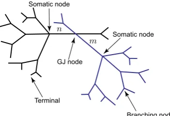
Fig. 10 A network of two cells as an extended tree structure with different types of nodes

L−1_[G

ij(x, y, ω)]. We consider a general case when each branch of the network can have different biophysical parameters and is characterised by the functionγk(ω)

defined as

γ2

k(ω)=_D1 k

1

τk +ω+

1

Ck(rk+ωLk)

, (28)

wherek labels an arbitrary branch of the network. Using the “sum-over-trips” for-malismGij(x, y, ω)can be constructed as an infinite series expansion

Gij(x, y, ω)=_D 1 jγj(ω)

trips

Atrip(ω)H_∞Ltrip(i, j, x, y, ω), (29)

whereH_∞(x)=e−|x|/2 andLtrip(i, j, x, y, ω)is the length of a path along the

on branchj. Note that the length of each branch of the network needs to be scaled byγk(ω)beforeLtripis calculated for (29). It is also worth mentioning here that if

all branches of a network have the same biophysical parameters, i.e.γk(ω)=γ (ω), the functionH_∞(Ltrip(ω))/(Dγ (ω))=G∞(Ltrip, ω)defined by (19). The trip

coef-ficientsAtrip(ω)in (29) are chosen according to the following set of rules:

• InitiateAtrip(ω)=1.

Branching node

• For any branching node at which the trip passes from branch i to a different branchk,Atrip(ω)is multiplied by a factor 2pk(ω).

• For any branching node at which the trip approaches a node and reflects off this node back along the same branchk,Atrip(ω)is multiplied by a factor 2pk(ω)−1.

Here, the frequency dependent parameterpk(ω)is defined as

pk(ω)=zk(ω)

nzn(ω), zk(ω)=

γk(ω)

ra,k , (30)

where the sum is over all branches connected to the node.

Terminal

• For every terminal which always reflects any trip,Atripis multiplied by+1 for the closed-end boundary condition or by−1 for the open-end boundary condition.

Somatic node

• For the somatic node at which the trip passes through the soma from branchito a different branchk,Atrip(ω)is multiplied by a factor 2ps,k(ω).

• For the somatic node at which the trip approaches the soma and reflects off the soma back along the same branch k, Atrip(ω) is multiplied by a factor

2ps,k(ω)−1.

Here, the frequency dependent parameterps,k(ω)is defined as

ps,k(ω)=

zk(ω)

nzn(ω)+γs(ω), γs(ω)=Csω+

1

Rs +

1

rs+Lsω, (31)

where the sum is over all branches connected to the soma.

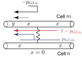
GJ node

• For the GJ node at which the trip passes through the gap junction from branchn to branchm,Atrip(ω)is multiplied by a factorpGJ,m(ω). For the GJ node at which the trip passes through the gap junction from branchmto branchn,Atrip(ω)is multiplied by a factorpGJ,n(ω).

• For the GJ node at which the trip approaches the gap junction, passes it and then continues along the same branch m, Atrip(ω) is multiplied by a factor 1−pGJ,n(ω). For the GJ node at which the trip approaches the gap junction, passes it and then continues along the same branchn,Atrip(ω)is multiplied by a

Fig. 11 A two-cell model

• For the GJ node at which the trip approaches the gap junction and reflects off the gap junction back along the same branchm,Atrip(ω)is multiplied by a factor

−pGJ,n(ω). For the GJ node at which the trip approaches the gap junction and

reflects off the gap junction back along the same branchn,Atrip(ω)is multiplied

by a factor−pGJ,m(ω).

Here, parameterspGJ,m(ω)andpGJ,n(ω)are defined by Eqs. (26) and (27).

We refer the reader to Coombes et al. [17] for a proof of rules for branching and somatic nodes. In AppendixB, we prove that the rules for generating the trip coeffi-cients at the GJ node satisfy the gap-junctional boundary conditions.

4 Application: Two-Cell Network

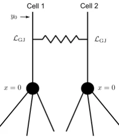
Here, we demonstrate how the “sum-over-trips” formalism can be applied to a two-cell network for obtaining insight into network response. As an example, we consider a model of two identical cells, each of which consists of a soma andN attached semi-infinite dendrites as shown in Fig.11. The cells are coupled by a dendro-dendritic gap junction located at some distanceLGJaway from their cell bodies. We assume

that this network receives an input at the locationy0. To study the dynamics of this

network, we use the “sum-over-trips” framework and construct the Green’s functions

G1(x, y0, ω)andG2(x, y0, ω)for Cell 1 and Cell 2, respectively.

4.1 Method of Words for Compact Solutions

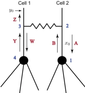
Here, we introduce a method which allows us to construct compact solution forms for the Green’s functions of this two-cell network. We describe this method in detail by constructing the Green’s functionG2(x0, y0, ω)for Cell 2 whenx0is placed between

the soma and the gap-junction as shown in Fig.12. Introducing points from 1 to 4 on this network, we associateletterswith different directions as follows:

• Fromx0→1 or from 2→1: letterA.

• Fromx0→2 or from 1→2: letterB.

Fig. 12 A two-cell model with associated letters

• From 4→3: letterY. • From 3→y0: letterZ.

Then the shortest trip which is a trip fromx0→2→3→y0is associated with the (ordered) word BZconsisting of one syllable. This and any trip associated with a word that starts with the letterB, i.e. fromx0→2, and ends with the letterZ, i.e. from 3→y0, will belong to class 1. Any trip associated with a word which starts fromx0→1→2 and ends with 3→y0, will belong to class 2. The shortest trip

in this class is associated with the wordABZ, consisting of two syllables, ABand

BZ. We introduce the following table that associates individual coefficients in the “sum-over-trips” framework with the syllables:

A B W Y Z

A 0 2ps(ω)−1 0 0 0

B −pGJ(ω) 0 pGJ(ω) 0 pGJ(ω)

W 0 0 0 2ps(ω)−1 0

Y pGJ(ω) 0 −pGJ(ω) 0 1−pGJ(ω)

Z 0 0 0 0 0

As the cells are identical in this network, the parameterpGJ(ω)is defined by (18) and

ps(ω)=

γ (ω)/ra

Nγ (ω)/ra+γs(ω), (32)

whereN is a number of dendrites attached to each soma andγs(ω)is given in (31).

Then, using the table, it is easy to conclude that for example, the word BZis as-sociated with the coefficient pGJ(ω) and the word ABZ, consisting of the

sylla-bles ABand BZ, is associated with the coefficient (2ps(ω)−1)pGJ(ω). We also

notice from the table that different coefficients are associated with the syllables

BZ and YZ and, therefore, we need to introduce two additional classes. Class 3 will include the trips with the main skeleton x0→2→ 3→4→3→ y0 and

the associated wordBWYZ. Class 4 will include the trips with the main skeleton

skeleton structures (the shortest words) of the four classes, we have

BZ+ABZ+BWYZ+ABWYZ= (1+A)BZ

class 1 and class 2

+(1+A)BWYZ

class 3 and class 4

. (33)

Any new word in each class can be formed by adding a combination of syllables

ABandWYinto the structure (33). Introducing such additions ofncombinations of syllables consisting ofksyllablesABand(n−k)syllablesWYby[· · · ](both syllablesABandWYcan take any position in this sequence ofnsyllables), class 3 and class 4 can be generalised as

(1+A)B[· · · ]WYZ

class 3 and class 4

. (34)

Similarly, we can generalise class 1 and class 2. However, to ensure that the words belong to class 1 and class 2, the syllableABmust be at the end of each word in combinations. This can be written as

(1+A)B[· · · ]Z

class 1 and class 2

, (35)

where

[· · · ]= 1+ [· · · ]AB. (36)

Using combinatorics, we can write

[· · · ] =

n

k=0

_n

k

(AB)k(WY)n−k

=

_n

0

(WY)n+

n−1

k=1

_n

k

(AB)k(WY)n−k+

_n

n

(AB)n, (37)

which leads to

[· · · ] =

_n

0

2ps(ω)−1n−pGJ(ω)n−1

+

n−1

k=1

_n

k

2ps(ω)−1k−pGJ(ω)k−1

×pGJ(ω)2ps(ω)−1n−k−pGJ(ω)n−k−1

+

_n

n

2ps(ω)−1

n

−pGJ(ω)

n−1

=

_n

0

2ps(ω)−1

n

−pGJ(ω)

−

n−1

k=1

_n

k

2ps(ω)−1

n_−p

GJ(ω)

n−1

+

_n

n

2ps(ω)−1n−pGJ(ω)n−1. (38)

Considering the possible trips in class 3 given by

B[· · · ]WYZ (39)

and substituting the expression for[· · · ]found in (38), we find

pGJ(ω)

_n

0

2ps(ω)−1

n

−pGJ(ω)

n−1

−pGJ(ω)

2ps(ω)−1

1−pGJ(ω)

−−pGJ(ω)

n−1

k=1

_n

k

2ps(ω)−1n−pGJ(ω)n−1

×−pGJ(ω)

2ps(ω)−1

1−pGJ(ω)

+−pGJ(ω)n n

2ps(ω)−1n−pGJ(ω)n−1

×pGJ(ω)

2ps(ω)−1

1−pGJ(ω)

= 2n2ps(ω)−1

n

−pGJ(ω)

n_p

GJ(ω)

2ps(ω)−1

1−pGJ(ω)

. (40)

Similarly, the possible trips in class 4 given by

AB[· · · ]WYZ (41)

generate the trip coefficients

2ps(ω)−1 2n

2ps(ω)−1

n

−pGJ(ω)

n_p

GJ(ω)

2ps(ω)−1

1−pGJ(ω)

. (42)

Expressions (40) and (42) for coefficients in the trips belonging to class 3 and class 4 can now be used in the “sum-over-trips” expansion (29) to obtain

∞

n=0

−2pGJ(ω)2ps(ω)−1npGJ(ω)2ps(ω)−11−pGJ(ω)

× G_∞y0−x0+2(n+1)LGJ, ω +2ps(ω)−1G∞

y0+x0+2(n+1)LGJ, ω

, (43)

whereG_∞(x, ω)=H_∞(γ (ω)x)/(Dγ (ω))defined by (19). Similarly, we can show that the possible trips in class 1 and class 2 given by

generate the terms

pGJ(ω)G∞(y0−x0, ω)+pGJ(ω)

2ps(ω)−1G∞(y0+x0, ω)

+

∞

n=0

−2pGJ(ω)2ps(ω)−1npGJ(ω)−pGJ(ω)2ps(ω)−1

× G_∞y0−x0+2(n+1)LGJ, ω

+2ps(ω)−1G∞

y0+x0+2(n+1)LGJ, ω

. (45)

Combining together (43) and (45), we obtain

G2(x0, y0, ω)=pGJ(ω)G_∞(y0−x0, ω)+pGJ(ω)2ps(ω)−1G∞(y0+x0, ω)

+∞

n=0

−2pGJ(ω)

2ps(ω)−1

n_p

GJ(ω)

2ps(ω)−1

×−pGJ(ω) G∞

y0−x0+2(n+1)LGJ, ω

+2ps(ω)−1G∞y0+x0+2(n+1)LGJ, ω +1−pGJ(ω) G∞

y0−x0+2(n+1)LGJ, ω

+2ps(ω)−1G∞

y0+x0+2(n+1)LGJ, ω

. (46)

Terms in{· · · }in (46) represent multiple trips in each of four classes and since there is a match in the length of trips among different classes, Eq. (46) can be simplified as

G2(x0, y0, ω)=pGJ(ω) G_∞(y0−x0, ω)+2ps(ω)−1G_∞(y0+x0, ω)

+∞

n=0

2n−pGJ(ω)

2ps(ω)−1

n+1

2pGJ(ω)−1

× G_∞y0−x0+2(n+1)LGJ, ω

+2ps(ω)−1G_∞y0+x0+2(n+1)LGJ, ω. (47)

Using this method of ‘words’, we can construct compact solution forms for the Green’s function for each of these two cells for any combinations of input,y, and output, x, locations. For example, placing x0 in Cell 1 between its soma and the

gap-junction we obtain

G1(x0, y0, ω)=1−pGJ(ω) G_∞(y0−x0, ω)+2ps(ω)−1G_∞(y0+x0, ω)

+∞

n=0

2n−pGJ(ω)

2ps(ω)−1

n+1

1−2pGJ(ω)

× G_∞y0−x0+2(n+1)LGJ, ω

Fig. 13 Values ofΩ0 at the soma of each cell as a function ofLGJ wheny0=LGJ+10 μm and

R_GJ=100 M(red circles),RGJ=1000 M(black crosses). Passive somas with parameters:

diame-teras=25 μm,Cs=1 μF/cm2,Rs=2000cm2. Resonant dendrites (N=4) with parameters given in

Fig.4

4.2 Network Dynamics

To study the role of a gap-junction in this two-cell network model, we focus on the Green’s functions at the somas of these two cells in response to a stimulus at the loca-tiony0. Using Eqs. (47) and (48), we obtain the following somatic response functions:

G1(0, y0, ω)=2ps(ω)

1−pGJ(ω)G∞(y0, ω)

+∞

n=0

2n−pGJ(ω)2ps(ω)−1n+11−2pGJ(ω)

×2ps(ω)G∞y0+2(n+1)LGJ, ω, (49)

and

G2(0, y0, ω)=2ps(ω)pGJ(ω)G∞(y0, ω)

+

∞

n=0

2n−pGJ(ω)2ps(ω)−1n+12pGJ(ω)−1

×2ps(ω)G_∞y0+2(n+1)LGJ, ω. (50)

Resonant properties of each cell are analysed by studying a preferred frequencyΩ0

for each cell. This is defined as the frequency at which the corresponding power function,P1(ω)= |G1(0, y0, ω)|2for Cell 1 andP2(ω)= |G2(0, y0, ω)|2for Cell 2,

reaches its maximum. This means thatΩ0for each soma is simply a solution of one of the corresponding equations,∂P1(ω)/∂ω=0 and∂P2(ω)/∂ω=0.

Fig. 14 Values ofΩ0 at the soma of each cell as a function ofLGJ wheny0=LGJ+10 μm and

R_GJ=100 M(red circles),RGJ=1000 M(black crosses). Resonant somas with parameters:

diam-eteras=25 μm,Cs=1 μF/cm2,Rs=2000cm2,rs=1cm2,Ls=0.1 H cm2. Passive dendrites

(N=4) with parameters given in Fig.4

Fig. 15 Values ofΩ0 at the soma of each cell as a function ofLGJ wheny0=LGJ+10 μm and

R_GJ=100 M(red circles),RGJ=1000 M(black crosses). Resonant somas with parameters:

diame-teras=25 μm,Cs=1 μF/cm2,Rs=2000cm2,rs=1cm2,Ls=0.1 H cm2. Resonant dendrites

(N=4) with parameters given in Fig.4

Fig. 16 Voltage profiles in the somas of cells in response to a stimulusIchirp(t)applied at the location

y_0=LGJ+10 μm. Cells’ parameters as in Fig.15,RGJ=100 M,ωchirp=0.003,Achirp=1 nA.Black

curves:LGJ=50 μm,green curves:LGJ=500 μm

5 Discussion

In this paper, we have generalised the “sum-over-trips” formalism for single dendritic trees to cover networks of gap-junction coupled resonant neurons. With the use of ideas from combinatorics, we have also introduced a so-called method of ‘words’ that allows for a compact representation of the Green’s function network response formulas. This has allowed us to determine that the position of a dendro-dendritic gap junction can be used to tune the preferred frequency at the cell body. Moreover we have been able to generate mathematical formula for this dependence without recourse to direct numerical simulations of the physical model. One clear prediction is that the preferred frequency increases with distance of the gap junction from the soma in a model with passive soma and resonant dendrites. In contrast for a system with a resonant soma and passive or resonant dendrite, the preferred frequency decreases as the gap junction is placed further away from the cell body.

network symmetries (either arising from the identical nature of the cells, their shapes, or the topology of their coupling) to allow for the compact representation of network response (and further utilising the method of ‘words’). Another is to incorporate a model of an active soma whilst preserving some measure of analytical tractability. Schwemmer and Lewis [21] have recently achieved this for a single unbranched cable model by coupling it to an integrate-and-fire soma model. The merger of our approach with theirs may pave the way for understandingspiking networks of gap junction coupled dendritic trees. Moreover, by using the techniques developed by them in [22] (using weakly coupled oscillator theory) we may further shed light on the role of dendro-dendritic coupling in contributing to the robustness of phase-locking in oscillatory networks.

Competing Interests

The authors declare that they have no competing interests.

Authors’ Contributions

YT, SC and DM contributed equally. All authors read and approved the final manuscript.

Acknowledgements YT would like to acknowledge the support provided by the BBSRC (BB/H011900) and the RCUK. DM would like to acknowledge the Complexity Science Doctoral Training Centre at the University of Warwick along with the funding provided by the EPSRC (EP/E501311).

Appendix A: Two Simplified Identical Cells with Passive Membrane

Equations (14)–(16) withγ2(ω)=(1/τ+ω)/Dprovide the solutions of a model in Fig.2with passive membrane. We introduce the function

F (x, ω, q)=_{γ (ω)}1 +q

e−γ (ω)|x|

2Dγ (ω), (51)

and its inverse Laplace transform

F (x, t, q)=L−1 _{F (x, ω, q)}

=1 2e

|x|q_e(q2_{D−1/τ )t}

erfc

q√D+ |x| 2√Dt

Θ(t). (52)

Then the Green’s function on each segment can be found in closed form as

G_m−(x, y, t)=L−1 Gm−(x, y, ω)

=_C1

G_∞(x−y, t)− ra 2RGJ

F (x+y, t, ra/R)

, (53)

=_C1

G_∞(x+y, t)− ra 2RGJ

F (x+y, t, ra/R)

, (54)

G_n±(x, y, t)=L−1 Gn±(x, y, ω)

=_C1

_r

a

2RGJ

F (x+y, t, ra/R)

, (55)

whereG_∞(x, t)is the Green’s function of the passive infinite dendritic cable,

G_∞(x, t)=L−1

e−γ (ω)|x| 2Dγ (ω)

=√ 1 4πDte

−t/τ_e−x2_/(4Dt)

Θ(t). (56)

If an external stimulusIinj,m−(x, t)=δ(x−y)I (t)has a form of a rectangular pulse withI (t)=η0Θ(t)Θ(τR−t), the voltage response on each segment can also be found in closed form:

Vm−(x, t)= B(x−y, t)−B(x−y, t−τR)

−P (x+y, t)−P (x+y, t−τR)/C, (57)

Vm+(x, t)= B(x+y, t)−B(x+y, t−τR)

−P (x+y, t)−P (x+y, t−τR)/C, (58)

Vn±(x, t)= P (x+y, t)−P (x+y, t−τR)/C, (59)

where

B(x, t)= η0

4√D/τ

e−|x|/ √

Dτ_erfc |x|

2√Dt −

t/τ

−e|x|/ √_Dτ

erfc _|x|

2√Dt +

t/τ

Θ(t), (60)

P (x, t)= η0ra

2DRGJ aF (x, t, ra/RGJ)+bF (x, t, √_ε)

+cF (x, t,−√ε), (61)

and

ε=_Dτ1 , a=_(r 1

a/RGJ)2−ε ,

b= 1

2√ε(√ε−ra/RGJ)

, c= 1

2√ε(√ε+ra/RGJ) .

(62)

These solutions generalise earlier results of Harris and Timofeeva [23] applicable to a neural network, but with gap-junctional coupling at tip-to-tip contacts of two branches.

Appendix B: Proof of the “Sum-over-Trips” Rules at the Gap Junction

Fig. 17 The GJ nodewith possible trips in its proximity

branch, say labelled byk, of the tree is re-scaled asX=γk(ω)x,x∈ [0,Lk]):

G_m−j(0, Y, ω)=Gm+j(0, Y, ω), (63)

G_n−j(0, Y, ω)=Gn+j(0, Y, ω), (64)

and

γm(ω)

ra,m

_∂G

m−j

∂X

_X

=0

+∂G_∂Xm+j

X=0

=gGJ

G_m−j(0, Y, ω)−Gn−j(0, ω), (65)

γn(ω)

ra,n

_∂G

n−j

∂X

_X

=0

+∂G_∂Xn+j

X=0

=gGJGn−j(0, Y, ω)−Gm−j(0, Y, ω). (66)

We prove here that the rules for generating the trip coefficients are consistent with these boundary conditions.

LetX denote the distance away from the GJ node along the segmentm− (see Fig.17). The location of the stimulusY =γj(ω)y, the segment number j and the variable ω are all considered to be arbitrary. Suppose that we sum all the trips starting from the GJ node itself and ending at point Y on branch j. We denote the result of summing over all trips that initially leave the GJ node along segment

m− _{byQm−j(0, Y, ω), along segmentm}+ _{byQm+j(0, Y, ω), along segmentn}− _by

Qn−j(0, Y, ω)and along segmentn+byQn+j(0, Y, ω).

Trips that start out fromXand move away from the GJ node are identical to trips that start out from the GJ node itself along segmentm−. The only difference is that the trips in the first case are shorter by the lengthX. We denote the sum of such shortened trips byQm−j(−X, Y, ω). The argument−Xmeans that a distanceXhas to be subtracted from the length of each trip summed to computeQ(and not that the trips start at the point−X).

according to the “sum-over-trips” rules. Therefore, the contribution to the solution

G_m−j(X, Y, ω) from those trips is −pGJ,n(ω)Qm−j(X, Y, ω). Trips that start out

from X by moving toward the GJ node and then continue moving along branch

m, i.e. on segmentm+, pick up a factor 1−pGJ,n(ω)and the sum of such trips is given by(1−pGJ,n(ω))Qm+j(X, Y, ω). Finally, trips that start fromX, move toward the GJ node and then leave the GJ node by moving out along segment n− or n+ pick up a factorpGJ,n(ω)and contribute to the solutionGm−j(X, Y, ω)by the terms

pGJ,n(ω)Qn−j(X, Y, ω)orpGJ,n(ω)Qn+j(X, Y, ω).

The full solutionGm−j(X, Y, ω)includes the contributions from all different types

of trips we have been discussing. Thus,

Gm−j(X, Y, ω)=_D 1

jγj(ω) Qm−j(−X, Y, ω)+

−pGJ,n(ω)Qm−j(X, Y, ω)

+1−pGJ,n(ω)

Qm+j(X, Y, ω)+pGJ,n(ω)Qn−j(X, Y, ω)

+pGJ,n(ω)Qn+j(X, Y, ω). (67)

The functionsQin this formula consist of infinite sums over trips, but we do not need to know what they are to show that the solutionGm−j(X, Y, ω)satisfies the GJ node boundary conditions. At the GJ node, we have

Gm−j(0, Y, ω)= 1

Djγj(ω) 1−pGJ,n(ω)

Qm−j(0, Y, ω)

+1−pGJ,n(ω)

Qm+j(0, Y, ω)

+pGJ,n(ω)Qn−j(0, Y, ω)+Qn+j(0, Y, ω). (68)

Considering the solutionGm+j(0, Y, ω) instead gives us the same expression as in

(68) and, therefore,Gm−j(X, Y, ω)obeys the boundary condition (63). Similarly, we can show that

Gn−j(0, Y, ω)=Gn+j(0, Y, ω)

=_D 1

jγj(ω) 1−pGJ,m(ω)

Qn−j(0, Y, ω)

+1−pGJ,m(ω)Qn+j(0, Y, ω)

+pGJ,m(ω)

Qm−j(0, Y, ω)+Qm+j(0, Y, ω), (69)

which satisfies the boundary condition (64).

To prove the boundary condition (65) we use Eq. (67) to find that

∂Gm−j

∂X

_X

=0

=_D 1

jγj(ω)

_∂Q

m−j(−X, Y, ω)

∂X

_X

=0

+1−pGJ,n(ω)

∂Qm+j(X, Y, ω)

∂X

_X

=0

+pGJ,n(ω)

_∂Q

n−j(X, Y, ω)

∂X

_X

=0

+∂Qn+j_∂X(X, Y, ω)

X=0

. (70)

Using the following properties for the termQkj(X, Y, ω),k∈ {m−, m+, n−, n+},

∂Qkj(X, Y, ω)

∂X = −Qkj(X, Y, ω), (71) ∂Qkj(−X, Y, ω)

∂X =Qkj(X, Y, ω), (72)

Eq. (70) can be simplified as

∂G_m−j

∂X

_X

=0

=1+pGJ,n(ω)Qm−(0, Y, ω)−1−pGJ,n(ω)Qm+(0, Y, ω)

−pGJ,n(ω)Qn−(0, Y, ω)+Qn+(0, Y, ω). (73)

Similarly,

∂G_m+j

∂X

_X

=0

=1+pGJ,n(ω)Qm+(0, Y, ω)−1−pGJ,n(ω)Qm−(0, Y, ω)

−pGJ,n(ω)Qn−(0, Y, ω)+Qn+(0, Y, ω). (74)

Substituting (73) and (74) together with (68) and (69) in Eq. (65) gives us the right equality. Similarly, we can prove the boundary condition (66).

References

1. Cajal R:Significación fisiológica de las expansiones protoplásmicas y nerviosas de la sustancia gris.Revista de ciencias medicas de Barcelona1891,22:23.

2. Segev I, Rinzel J, Shepherd GM (Eds):The Theoretical Foundations of Dendritic Function: Selected Papers of Wilfrid Rall with Commentaries. Cambridge: MIT Press; 1995.

3. Mainen ZF, Sejnowski TJ:Influence of dendritic structure on firing pattern in model neocortical neurons.Nature1996,382:363-366.

4. van Ooyen A, Duijnhouwer J, Remme MWH, van Pelt J:The effect of dendritic topology on firing patterns in model neurons.Network2002,13:311-325.

5. Spruston N, Stuart G, Häusser M:Dendritic integration. InDendrites. New York: Oxford University Press; 2008.

6. Hormuzdi SG, Filippov MA, Mitropoulou G, Monyer H, Bruzzone R:Electrical synapses: a dy-namic signaling system that shapes the activity of neuronal networks.Biochim Biophys Acta 2004,1662:113-137.

7. Bennet MVL, Zukin RS:Electrical coupling and neuronal synchronization in the mammalian brain.Neuron2004,41:495-511.

9. Traub RD, Whittington MA, Buhl EH, LeBeau FEN, Bibbig A, Boyd S, Cross H, Baldeweg T:A pos-sible role for gap junctions in generation of very fast EEG oscillations preceding the onset of, and perhaps initiating, seizures.Epilepsia2001,42(2):153-170.

10. Nakase T, Naus CCG:Gap junctions and neurological disorders of the central nervous system. Biochim Biophys Acta, Biomembr2004,1662(1–2):149-158.

11. Söhl G, Maxeiner S, Willecke K:Expression and functions of neuronal gap junctions.Nat Rev, Neurosci2005,6:191-200.

12. Bem T, Rinzel J:Short duty cycle destabilizes a Half-Center oscillator, but gap junctions can restabilize the anti-phase pattern.J Neurophysiol2004,91:693-703.

13. Traub RD, Kopell N, Bibbig A, Buhl EH, LeBeau FEN, Whittington MA:Gap junctions between interneuron dendrites can enhance synchrony of gamma oscillations in distributed networks. J Neurosci2001,21:9478-9486.

14. Saraga F, Ng L, Skinner FK:Distal gap junctions and active dendrites can tune network dynamics. J Neurophysiol2006,95:1669-1682.

15. Abbott LF, Fahri E, Gutmann S:The path integral for dendritic trees.Biol Cybern1991,66:49-60. 16. Abbott LF:Simple diagrammatic rules for solving dendritic cable problems.Physica A1992,

185:343-356.

17. Coombes S, Timofeeva Y, Svensson CM, Lord GJ, Josic K, Cox SJ, Colbert CM:Branching den-drites with resonant membrane: a “sum-over-trips” approach.Biol Cybern2007,97:137-149. 18. Hutcheon B, Miura RM, Puil E:Models of subthreshold membrane resonance in neocortical

neu-rons.J Neurophysiol1996,76:698-714.

19. Magee JC:Dendritic hyperpolarization-activated currents modify the integrative properties of hippocampal CA1 pyramidal neurons.J Neurosci1998,18:7613-7624.

20. Mauro A, Conti F, Dodge F, Schor R:Subthreshold behavior and phenomenological impedance of the squid giant axon.J Gen Physiol1970,55:497-523.

21. Schwemmer MA, Lewis TJ:Bistability in a leaky integrate-and-fire neuron with a passive den-drite.SIAM J Appl Dyn Syst2012,11:507-539.

22. Schwemmer MA, Lewis TJ:The robustness of phase-locking in neurons with dendro-dendritic electrical coupling.J Math Biol2012. doi:10.1007/s00285-012-0635-5.