Efficiency in contamination free machining using microfluidic structures

Manuscript version: Author’s Accepted Manuscript

The version presented in WRAP is the author’s accepted manuscript and may differ from the published version or Version of Record.

Persistent WRAP URL:

http://wrap.warwick.ac.uk/130973

How to cite:

Please refer to published version for the most recent bibliographic citation information. If a published version is known of, the repository item page linked to above, will contain details on accessing it.

Copyright and reuse:

The Warwick Research Archive Portal (WRAP) makes this work by researchers of the University of Warwick available open access under the following conditions.

© 2019 Elsevier. Licensed under the Creative Commons Attribution-NonCommercial-NoDerivatives 4.0 International http://creativecommons.org/licenses/by-nc-nd/4.0/.

Publisher’s statement:

Please refer to the repository item page, publisher’s statement section, for further information.

Efficiency in contamination-free machining using

microfluidic structures

Carlo Ferria,1

, Timothy Mintona,_∗

, Saiful Bin Che Ghania,2

, Kai Chenga

a

Brunel University, AMEE - Advanced Manufacturing and Enterprise Engineering, Kingston Lane, Uxbridge, Middlesex, UB8 3PH, UK

Abstract

The plastic deformation of the material in the chip formation and the friction

when the chip slides on the rake face of the insert generate heat. The heat

generation is responsible for a temperature rise of the chip, of the insert and of

the newly created surface on the workpiece. Adhesion and diffusion between

the chip and the insert are thus facilitated with detrimental effects on the

tool wear. A cooling system based on microfluidic structures internal to the

insert is considered in this study as a means of controlling the temperature

at the chip-insert interface. The coolant and the part never enter in contact.

Hence contamination of the part by coolant molecules is prevented. The

aim of this study is to identify and to quantify the effect of the cutting

parameters on the effectiveness of the internal cooling system. To measure

this effectiveness an efficiency ratio r is defined as the percentage of the

∗_{Corresponding author. Tel.: +44 1895 267945; fax: +44 1895 267583.}

Email address: [email protected](Timothy Minton) 1_{Present address: Via XI Febbraio 40, 24060 Castelli Calepio, BG, Italy}

mechanical power actually needed at the tool to remove material that is

thermally dissipated by the internal flow of the coolant. Similarly, a specific

efficiency ratio r’ is also defined by considering the mechanical power per

volume flow rate of the material removed and the dissipated thermal power

per volume flow rate of the coolant. Both r andr’ are then analysed in a 33

factorial experiment within the space of the technological variables depth of

cut, feed rate and cutting speed. The cutting trials were conducted in turning

operations of AA6082-T6 aluminium alloy. Linear Mixed-effects models were

fitted to the experimental results using the maximum likelihood method. The

main finding was that the efficiency ratior depends only on the feed rate and

the cutting speed but not on the depth of cut. An interaction effect of the

feed rate and the cutting speed on the efficiency was also found significant.

Higher efficiency is attainable by decreasing cutting speed and feed rate.

The maximum efficiency predicted in the technological region investigated

was 10.96 %. The specific efficiency once log-transformed was found linearly

increasing with the depth of cut and the feed rate, whereas being insensitive

to the cutting speed.

Keywords: Cutting temperature, internally-cooled tool, contamination-free

machining, dry machining, Linear mixed-effects statistical models

1. Introduction

1

Dry cutting of key engineering materials is the epitome of sustainability in

2

metal cutting. The removal of metal working fluids (MWF) from the

ma-3

chining processes is of benefit to the machine operator, swarf recycling and

4

ultimately the environment. Reducing the temperature of the cutting tool

and workpiece is one of the main purposes of the MWF, together with

facil-6

itating the removal of the chip from the machining area. Using an external

7

supply of coolant makes it difficult for the fluid to penetrate into the tool-chip

8

contact area. It is also difficult to quantify the amount of heat transferred

be-9

tween the cutting edge and the MWF. Dry machining removes the externally

10

supplied coolant from the machining process at the expense of the cooling

11

effect it provides. Although this method is acceptable for certain materials

12

like aluminium, it may be problematic for high strength materials and

cer-13

tain grades of aluminium which contain harder elements like silicon. High

14

temperatures which are uncontrolled due to lack of cooling can cause high

15

wear rates and can dramatically reduce the useful life of the tooling insert.

16

In some extreme cases the tool can become damaged not via traditional wear

17

mechanisms but through deformation of the cutting edge [1]. Monitoring

18

of the cutting temperature is a well-established research goal and has been

19

presented using many differing technologies including an embedded

thermo-20

couple [2], the tool-work thermocouple [3], the calorimetric method [4], an

21

embedded sensor film [5] and optical methods [6, 7]. Some of these methods

22

are not applicable when using an external coolant supply. Dry machining

23

allows the monitoring of the tool/chip temperature via the tool-work

ther-24

mocouple [3] or optical methods [6, 7]. These methods however require time

25

consuming setups or expensive auxiliary equipment and are hence better

26

suited to a laboratory environment.

27

The method of indirect cooling is known in the area of metal cutting and has

28

been steadily increasing in popularity since 1970 when Jefferies published the

29

idea of an internally cooled single-point cutting tool [8]. The main benefit

of the internally cooled tool is the indirect application of a cooling effect

31

to the tool-chip interface. Previous research in the field of indirect cooling

32

methods has shown that it is possible to reduce significantly the cutting

tem-33

perature. In particular, Ferri et al.[9] compared the chip temperature in dry

34

turning of the aluminium alloy AA6082-T6 when using conventional and

in-35

ternally cooled tools. Their main finding was that the internally-cooled tools

36

appeared increasingly effective in containing the chip temperature while

in-37

creasing the depth of cut. In a research effort jointly sponsored by the US

38

Environmental Protection Agency and the Department of the Army, Rozziet

39

al. [10] patented a device to cool indirectly the tool-chip interface by

creat-40

ing micro-channels and a finned heat exchanger within the tool suitable for

41

the use with cryogenic fluids (typically liquid Nitrogen). Sanchez et al. [11]

42

proposed a similar apparatus where the cooling fluid flowing within the tool

43

evaporates in proximity of the cutting edge, with the latent heat being

pro-44

vided by heat transfer with the tool-chip interface. In a condenser outside

45

the tool holder, the fluid is then condensed again. The resulting liquid phase

46

is re-conveyed within the tool, thus realising a close-loop circulation of the

47

coolant. Liang et al.[12] studied the use of the heat pipe technology in

turn-48

ing operations. A heat pipe is a heat conductor in which the latent heat

49

of evaporation is used for heat transfer purposes in experimental situations

50

where differences in temperature are small. Moreover, a heat pipe operates

51

without any external power supply. Shu et al. [13] presented a study based

52

on the finite element method to simulate numerically turning operations in

53

presence of both liquid coolant flowing in channels internal to the tool and a

54

heat pipe. Uhlmann et al.[14] compared wet machining, dry machining and

machining with an internally-cooled tool. They investigated the influence

56

of different coolant temperatures on the tool flank wear (VB) and on the

57

workpiece surface roughness. Their main finding is that the tool wear in dry

58

machining appears larger than in the other cases. They tested

internally-59

cooled tools with coolant temperatures of 20 ◦_{C and -10} ◦_{C. The tool flank} 60

wear in both these cases and in the wet machining were most similar. The

61

internally-cooled tool with coolant at 20 ◦_{C appeared only slightly less worn} 62

(cf. figure 3 in Uhlmann et al. [14]).

63

Moreover, internally cooling the tool also provides the unique possibility

64

to manipulate the cutting temperature without necessarily changing core

65

machining parameters such as the cutting speed, the feed rate or the depth

66

of cut. Whilst specifically focusing on a closed loop coolant supply within

67

the tool shank, the introduction of two additional control variables such as

68

the coolant supply flow rate and the coolant temperature can be deployed to

69

affect the metal removal process. The concept of a coolant supply within the

70

cutting tool itself also presents a great opportunity to quantitatively assess

71

the thermal energy that the coolant conveys away from the cutting zone. The

72

metal cutting process generates high heat and large thermal gradients [3].

73

According to Micheletti (cf page 203 in [15]), heat is almost instantaneously

74

generated where work is done during cutting. Thus, the location of the heat

75

sources is identified in the areas where the work due to the plastic deformation

76

of the metal and to the friction of the chip on the rake face happen. If the

77

tool is not in ideal conditions, i.e. if it is not perfectly sharpened, friction

78

work also happens between the surface of the workpiece and the clearance

79

face of the tool (also known as flank face) [15]. Boothroyd [16] measured the

temperature distribution and constructed isotherm patterns in the workpiece,

81

the chip and the tool by making joint usage of infra-red photography and

82

thermocouples. From those measurements, Boothroyd was also able to derive

83

the heat transferred into the chip, the tool and the workpiece. Boothroyd’s

84

results, displayed in the table on page 797 in [16], appear consistent with

85

those reported by Micheletti (cf page 209 in [15]): most of the heat generated

86

during the cutting process is transferred into the chip, say about 60 and 80

87

%, depending on the machining conditions; the remaining part is transferred

88

into the tool and into the workpiece in similar proportions.

89

When the coolant flows internally to the insert and close to the cutting edge,

90

a part of the generated heat is transferred into the coolant and away from the

91

cutting zone. The heat transfer occurred is evidenced through the increment

92

of the coolant temperature which is also instrumental to its measurement.

93

This can all be achieved without the contamination of the tool and of the

94

workpiece which instead occurs with external coolant supplies. For this

rea-95

son the authors used in the title and elsewhere the terms ‘contamination-free

96

machining’. At first sight, this may appear as an oxymoron. In fact, for

97

a metal cutting process to happen a tool must enter in contact with the

98

workpiece. The cutting edge of the insert must be harder than the material

99

to cut. Thus cutting edge and workpiece are of different materials. It is a

100

reasonable expectation that during the cutting process a proportion of the

101

material worn off the flank face (clearance face) of the tool will contaminate

102

the workpiece at least on a sub-micrometre scale. Thus, strictly speaking, as

103

long as flank wear exists on the tool, a cutting process is always most likely

104

to pollute the workpiece with tool material. The term ‘contamination-free’

is therefore to be considered within these limitations.

106

In some cases reducing the temperature of the workpiece or cutting insert

107

by too great a margin might be a problem. For example, if there is a strong

108

work-hardening effect on the material the cutting forces may increase

dra-109

matically and induce additional issues with the surface finish and the surface

110

integrity [17]. Another issue might be a thermal shock of the cutting insert.

111

However, the manipulation of the coolant flow rate and/or the coolant

tem-112

perature would make the management of these events possible. The benefits

113

of a reduced cutting temperature appear to out-weigh the potential

trou-114

bles by far. An increase in tool life is possible and a control of the critical

115

temperature above which thermally induced wear mechanisms take place is

116

achievable [18]. In this study, a tool system is designed and manufactured to

117

cool the cutting insert by the adduction of the coolant in the proximity of the

118

cutting insert via microfluidic structures within the tool. These structures

119

prevent any possible contact between the coolant and the part. A cooling

120

efficiency ratio is then defined and computed in a range of experimental

con-121

ditions defined by the triplets of machining parameters cutting speed (vc), 122

feed rate (f) and depth of cut (ap). This efficiency ratio denotes the portion 123

of the total machining power which is transferred to the coolant in the form of

124

thermal power. From a conceptual point of view, establishing experimentally

125

how this efficiency ratio depends on (ap, f, vc) provides other researchers a 126

further potential means of validating their theories regarding the thermal

127

characteristics of the machining process. From a practitioner’s point of view,

128

this efficiency ratio can become a useful instrument in the selection of the

129

coolant flow rate and coolant temperature at the inlet of the tool system. For

example, cutting speed, feed rate and depth of cut may be set to comply with

131

productivity requirements and/or the optimisation of some cost function. By

132

setting the triplet (ap, f, vc), the power request for machining a given ge-133

ometry from a given blank is uniquely determined. The knowledge of the

134

efficiency ratio of the cooling system for the selected triplet (ap,f,vc) allows 135

then the practitioner to know how much thermal power would be transferred

136

away by the cooling system, had he or she set the flow rate and the inlet

137

temperature of the coolant to the same values of this investigation. Prior to

138

any actual machining, the efficiency ratio can therefore suggest to the

prac-139

titioner whether the flow rate and the inlet temperature of the coolant may

140

need increasing or decreasing in order to balance the mechanical power and

141

have a thermally steady machining condition. More in general, this study of

142

the efficiency ratio may constitute a stepping stone towards the formulation

143

of a performance objective function (e.g. cost, profit) to be optimised in the

144

newly established penta-dimensional technological space of depth of cut, feed

145

rate, cutting speed, coolant flow rate and coolant inlet temperature.

146

2. Experimental set-up

147

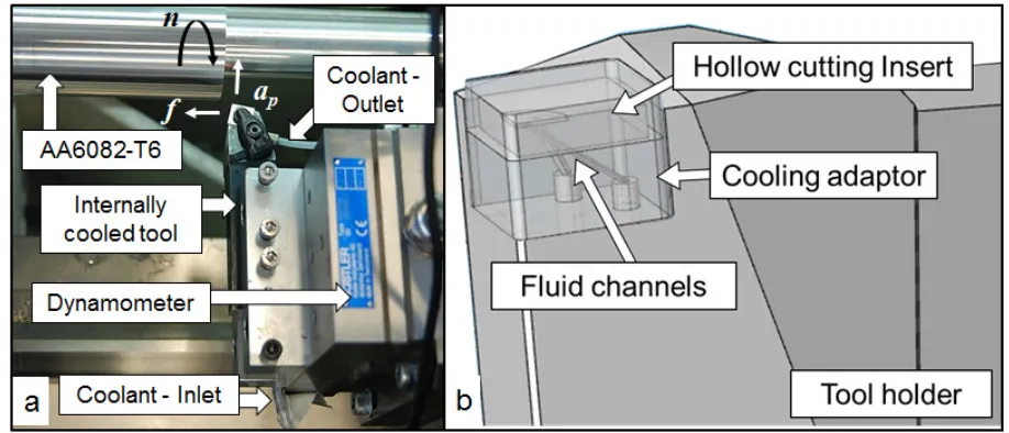
The tool has been assembled and secured to a dynamometer as shown in

148

Figure 1. The dynamometer was a three component Kistler type 9257B

149

which had been attached to the tool turret of an Alpha Colchester Harrison

150

600 Group CNC lathe.

151

[Figure 1 about here.]

The workpiece material chosen for this study was Aluminium 6082-T6

(0.7-153

1.3 % Si and 0.6-1.2 % Mg). This aluminium alloy is readily available and

154

widely used in numerous applications, an additional benefit is the low

me-155

chanical property demands on the tooling insert and therefore yields a low

156

wear rate. A cylindrical workpiece of 65 mm diameter and 450 mm length

157

was used. The internally cooled tool was enhanced in its measuring

capabil-158

ity by mounting K-type thermocouples. These were installed within the inlet

159

and the outlet pipes, close to where these pipes enter the tool body. These

160

sensors measured the inlet/outlet coolant temperatures. They were linked to

161

a PC via a National Instruments NI 9213 thermocouple input device. Data

162

from the thermocouples and the dynamometer were collected and transferred

163

to Labview prior to the analysis.

164

The internally cooled tool was comprised of the tool shank, a cooling adaptor

165

and a hollow insert, as shown in Figure 1. The tool shank was an off the

166

shelf model manufactured by Sandvik (CSBNR 2525M 12-4) which had been

167

enhanced with designed fluid channels machined inside it. The adaptor block

168

has been custom machined in mild steel. The cutting inserts were once

169

again an off the shelf -item produced by Hertel (SNUN 120408, Tungsten

170

Carbide WC with 6 % Cobalt). These were modified using electro discharge

171

machining to create a hollow with a 1 mmwall thickness. The coolant was

172

flowing from a central reservoir which contains approximately one litre of

173

coolant. From here it flowed through silicone tubing to a micro-diaphragm

174

pump from KNF-Neuberger (NFB 60 DCB). Upon exiting the pump, the

175

coolant then flowed to and around the part of the circuit enclosed within the

176

tool and finally back to the reservoir.

The volume flow rate of the coolant (Q) was approximately 0.3 L/min for all

178

the tests, i.e. in SI units Q = 0.3/60 000 m3_{/s. The coolant was a 25 % in} 179

volume liquid solution of Ethylene Glycol in water. The specific heat (Cp) 180

and the density (ρ) of the coolant were considered essentially constant and

181

approximately equal to 3850 J/kg K and 1040 kg/m3_{, respectively. The} 182

choice of using a 25 % Ethylene Glycol aqueous solution rather than water

183

was conservatively made to benefit from the ebullioscopic elevation of the

184

boiling point of the mixture. A bi-phase vapor-liquid flow within the

inter-185

nal microfluidics structures is in this way slightly less likely to take place.

186

This choice however adversely affects the efficiency of the cooling system.

187

For the same volume flow rate and for the same increment of temperature,

188

a coolant comprised of the Ethylene Glycol solution would exchange heating

189

power with the insert less than water would do. In the range of the tested

ex-190

perimental conditions, clean water has in fact comparable density but higher

191

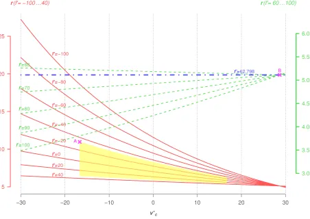
specific heat than the mixture used (approximately ρwater = 1000 kg/m3 and 192

Cp,water = 4184 J/kg K , albeit they both are not constant).

193

3. Design of the Experiment

194

The temperature of the coolant at the inlet (Tin) and at the outlet (Tout) 195

of the insert, together with the cutting and the thrust forces (Fc and Ft, 196

respectively) were measured in a set of experimental conditions defined by

197

three technological variables: the depth of cut (ap), the feed rate (f) and 198

the cutting speed (vc). These variables assume numerical values. They have 199

been therefore considered as continuous rather than categorical variables.

Each variable was assigned three values (Table 1). Thus a limited region was

201

identified in the space (ap, f, vc). 202

[Table 1 about here.]

203

Cutting trials were performed in the resulting 33

experimental conditions

204

(treatments). In each treatment, the cutting test was replicated three times.

205

thus the total number of tests accrued to 81. A unique label was given

206

to each treatment. Then, a permutation of the 27 labels was randomly

207

generated out of 27! possible label permutations. The treatments were run

208

in the order defined by such a permutation. All the three cutting trials

209

for a given treatment were performed in the same machine set-up. A full

210

randomisation of the cutting tests would have requested a new machine

set-211

up (different or equal to the latest) for each single cutting test. The set-up

212

time of the machine made a full randomisation of the 81 tests impracticable.

213

4. Modelling and Analysis

214

The thermal power exchanged between the coolant and the insert during

ma-215

chining ( ˙Q) causes the temperature of the coolant at the insert outlet (Tout) 216

to be higher than at the insert inlet (Tin, which is approximately equal to the 217

ambient temperature). By the application of the first law of thermodynamics

218

to the open system made of the coolant flowing in the microfluidic structures

219

within the insert, the following equation is derived for the steady state:

220

˙

From the measurements of the cutting force (Fc) and the thrust force (Ft), the 221

cutting powerPc =Fc (vc/60) and the thrust powerPt=Ft (f /1000) (n/60) 222

were calculated. In these expressions, n denotes the angular speed of the

223

blank in revolutions per minute, whereas the other coefficients have been

224

introduced to express the power in watt. To explore the relationship between

225

the efficiency of the internally-cooled tool and the machining conditions, a

226

definition of efficiency ratio r is introduced as follows:

227

r = 100 Q˙

Pc+Pt

(2)

In equation (2), the efficiency ratio r represents the percentage of the power

228

needed to remove material from the blank that is thermally transferred by the

229

flow of the internal coolant. Alternatively, r can be described as the scaled

230

ratio of the heat transfer rate associated with the flow of the coolant and the

231

mechanical power used at the tool to remove material from the workpiece.

232

In other words, The coefficient r does not represent some measurement of

233

efficiency of the cutting process, but a measurement of efficiency of the

in-234

ternal cooling system. The idea behind this approach is that the internal

235

cooling apparatus is more efficient the more thermal power it can remove

236

from the system tool/chip/workpiece per unit of power in input to such a

237

system, regardless of how this input power is then distributed between the

238

workpiece, the chip and the tool. In this view, the efficiency of a machine

239

tool in converting electrical power into mechanical power available at the tool

240

is also not relevant.

241

A specific efficiency ratio r’ is also introduced as follows:

242

Ps =

Pc+Pt

(ap/1000) (f /1000) (vc/60)

r′ _{= 100}Q/Q˙

Ps

(4)

The numerical coefficients in Equation (3) were introduced to convert the

243

measured technological variables to the si _{units (m, m/rev and m/s). In} 244

equation (4), the ratio r’ represents the percentage of the total machining

245

power per unit of volume (m3_{) of material removed from the blank in the unit} 246

of time (s) that is thermally dissipated by a unit of volume flow rate (m3_/s) 247

of the coolant. Both the dimensionless ratios r and r’ have been considered

248

as two response variables separately analysed. The measuring procedure for

249

r and r’ is the same for all the treatments.

250

Improving the efficiency merit by increasing the coolant mass flow rate ( ˙m=

251

Qρ), by identifying more efficient coolant fluids (with higher Cp), by refrig-252

erating the coolant (i.e. reducing Tin in Equation (1)) are all actions that 253

can be thought of, but that were not within the scope of this study. Hence

254

such actions were not taken. For example, the usage of cryogenic media such

255

as nitrogen and carbon dioxide has been reported in other cooling systems

256

such as high pressure jet cooling systems (cf page 311 – 338 in [19]).

Op-257

posite to the internally-cooled tool presented in this investigation, in those

258

systems the cryogenic coolant is a consumable: it evaporates rather than

259

being re-circulated in a closed-loop.

260

The parameters involved in the construction of a statistical model may

261

have desirable statistical proprieties if the independent variables are centred

262

around zero. Typically, intercepts and slopes are more likely to be

uncorre-263

lated if the independent variables are centred (cf. for example Pinheiro and

264

Bates [20], page 34). Also, dimensionless independent variables facilitate the

transformation of the data, which is often necessary in the construction of a

266

model. For these reasons, dimensionless, centred, independent variables were

267

defined as follows:

268

a′

p = 100

ap−0.35

0.35 ; f

′ _{= 100}f−0.15

0.15 ; v

′

c = 100

vc−300

300 (5)

The equations (5) define the per cent deviations from the central point

269

(ap,c, fc, vc,c) = (0.35 mm, 0.15 mm/rev, 300 m/min), which is the centre of 270

the investigated region in the space of the technological variables.

271

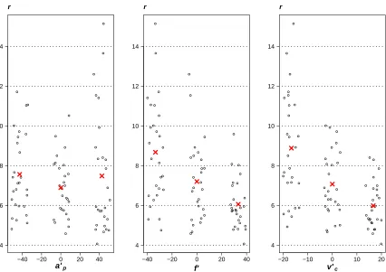
[Figure 2 about here.]

272

The diagram of the ratio r versusa′

p, f′ and vc′ is displayed in Figure 2. The 273

abscissae of the data have been increased by a random amount to avoid

over-274

lapping points and thus increasing the readability of the figure (a procedure

275

called jittering). In the same figure the sample mean of the data for each

276

value of the pertinent independent variable has been designated by a cross.

277

A qualitative visual analysis of Figure 2 raises the suspicion that the

dimen-278

sionless depth of cut a′

p does not significantly affect the efficiency ratio r, 279

whereas the dimensionless feed rate f′ _{and the dimensionless cutting speed} 280

v′

c may do. When either f′ or vc′ increases the efficiency ratio r’ appears to 281

deteriorate. Also, the variability ofr may be significantly inflated at higha′

p,

282

low f′ _{and low v}′

c. Interaction plots (not shown here for brevity) were also 283

constructed but they did not exhibit any pattern either strongly pointing to

284

or strongly ruling out any significant second order interaction.

285

Running the experiment in 27 experimental units (alias blocks), each

coin-286

cident with a treatment, suggests introducing a random effect in the model

to account for physical events or circumstances that may lurk within an

ex-288

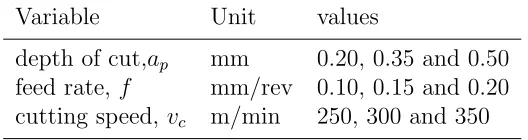
perimental unit while the tests are performed. For example, the portion of

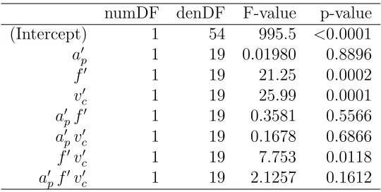
289

the blank being machined in an experimental unit may have micro-structural

290

and mechanical proprieties slightly different from those of other experimental

291

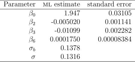
units. Without the introduction of a random effect, the likely effect of these

292

properties on the measured response would then be unduly attributed in part

293

to the independent variables.

294

A preliminary tentative model of the experimental data is as follows:

295

rijkl =β0+β1a′p,i+β2fj′+β3vc,k′ +β4a′p,ifj′+β5a′p,iv′c,k+β6fj′v′c,k+β7a′p,ifj′vc,k′ +bijk+εijkl

(6)

where the subscripts i = 1, . . . ,3, j = 1, . . . ,3, k = 1, . . . ,3 and l = 1, . . . ,3

296

represent the different depths, feed rates, cutting speeds and replications

297

of the tests, respectively. The β’s are eight unknown parameters of the

298

model, bijk’s are the 27 non-observable random variables associated with the 299

corresponding experimental units, εijkl are the 81 non-observable random 300

variables that model the random error. It is then assumed that all the random

301

variables in equation (6) are independent, identically distributed and normal

302

with constant variance, namely: bijk ∼ N(0, σb2), εijkl ∼ N(0, σ2), where 303

the standard deviationsσb and σ are two further unknown parameters of the 304

model. Under these assumptions, the ten model parameters are estimated

305

using the maximum likelihood method (ml_{) as implemented in the library}

306

nlme _{[21, 20] of} r_{, a free language and run-time environment for statistical} 307

computing and graphics [22]. The significance of the terms associated to the

308

technological variables that enter Equation (6) by the β’s has been tested

309

sequentially in the order they appear in the model and conditionally on the

estimate of σb (cf. Pinheiro and Bates [20], 89-92). A term is added in the 311

model only if such an inclusion reduces significantly the variability of the

312

predicted errors. The test was performed using the anova() _{function of the}

313

nlme _library.

314

[Table 2 about here.]

315

The results of the tests displayed in Table 2 support the conclusion that

316

Equation 6 does not fit the data any better than the following simpler model

317

equation, which is thus to be preferred:

318

rijkl =β0+β2fj′ +β3vc,k′ +bijk+β6fj′vc,k′ +εijkl (7)

The library nlme _{allows the experimenters to predict the observed response}

319

values by the fitted model, both at population level, i.e. ˆE [rijkl] = ˆE [rij] = 320

ˆ

β0+ ˆβ2f_j′+ ˆβ3v_c,k′ + ˆβ6f_j′v′_c,kand at experimental unit level, i.e. ˜E [rijkl|bijk] = 321

˜

E [rijk|bijk] = ˆβ0 + ˆβ2fj′ + ˆβ3v_c,k′ + ˆβ6fj′vc,k′ + ˜bijk (with E[X] designating 322

the expected value of X, ˆα the estimate of the parameter α and ˜X, the

323

predictor of the random variable X). In this second case, the best linear

324

unbiased predictors ˜bijk of the random effects are also calculated (BLUEs, 325

cf. Pinheiro and Bates [20], 94). In turn, predictions of the non-observable

326

errors can thus be computed and are usually referred to as residuals, namely:

327

˜

εijkl = rijkl −E [˜ rijk|bijk]. Departures from the hypotheses underlying the 328

model are diagnosed by the graphical analysis of the residuals.

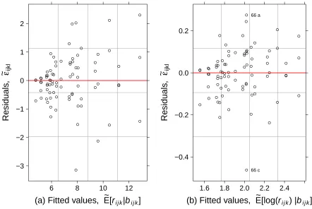
329

[Figure 3 about here.]

330

In part (a) of Figure 3 the dispersion of the residuals around the zero appears

331

to increase with the values fitted by the model of Equation (7). Such an

observation is inconsistent with the assumed equal variance of the errors (σ2_). 333

To overcome the violation of this hypothesis, the response is logarithmically

334

transformed in the following new model:

335

log(rijkl) =β0+β2fj′+β3vc,k′ +β6fj′vc,k′ +bijk+εijkl (8)

An equivalent representation of equation (8) is given by its multiplicative

336

form:

337

rijkl =eβ0eβ2f

′

jeβ3v′_c,k

eβ6f_j′vc,k_ebijk_eεijkl ₍₉₎

More details regarding suitable transformations of the response to overcome

338

observed departures of the assumed homoscedasticity of the errors in the

339

case of linear models are presented by Faraway (cf pages 53–58 in [23]). The

340

parameters in Equation (8) and (9) have been estimated as in the previous

341

cases using thenlme _{library (Table 3). The adequacy of the fitted model has}

342

been assessed with the Akaike Information Criterion (AIC), formally defined

343

by AIC =−2 logLik + 2npar, where logLik = 29.70 is the log-Likelihood of 344

the fitted model (i.e. the maximum log-Likelihood) andnpar= 6 is the num-345

ber of parameters estimated in the model, thus AIC =−47.39 (cf Pinheiro

346

and Bates [20], pages 10, 83, 84).

347

[Table 3 about here.]

348

In part (b) of Figure 3 the residuals of the model involving the log-transformed

349

efficiency ratio r appear to have a dispersion around zero that is markedly

350

less dependant on the fitted values than in the original model with

untrans-351

formed response (part (a) of Figure 3). Also, two residuals labelled ‘66 a’

352

and ‘66 c’ in part (b) of the same figure are noticeably lying quite far apart

from the majority of the others. The two labels indicate that these two

resid-354

uals have been obtained as the first and third replicate of the treatment 66,

355

which corresponds to ap = 0.5 mm, f = 0.1 mm/rev and vc = 300 m/min 356

(a′

p = 42.86, f′ = −33.34, vc′ = 0). No specific reason has been identified 357

for the two associated experimental results to cause this outlying situation.

358

Thus there was no reason for excluding the two experimental results from

359

the analysis. Moreover, even doing so, the resulting fitted model did not lead

360

to significantly different estimates of the parameters. Namely, the confidence

361

intervals for corresponding parameters in the two models were overlapping.

362

The fact that these two residuals were obtained in the same experimental

363

unit instils the suspicion that the uncontrollable unknown reason causing

364

the outlying of the two residuals may be related to the specific experimental

365

unit. In this sense, the two outlying residuals reinforce the motivations for

366

introducing the random effects bijk in the model of the experimental results. 367

Without random effects as in the following model equation:

368

log(rjk) = β0+β2f_j′ +β3v′_c,k+β6f_j′v_c,k′ +εjk (10)

the residuals appear inconsistent with the assumption of errors (εijkl) char-369

acterised by zero mean and equal variance.

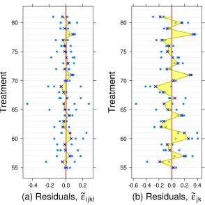
370

[Figure 4 about here.]

371

In Figure 4, when the random effects bijk are part of the model (cf. part (a) 372

of the figure), the three residuals corresponding to each experimental

condi-373

tion (treatment) have a sample mean that is close to zero. Otherwise, they

374

have not (cf. part (b) of the figure). The deviation of such a sample mean

375

from zero is what the random effect of a treatment is specifically meant to

account for. Moreover, in part (b) of the figure, 15 of these sample means

377

are negative, whereas 12 are positive. This symmetry in the distribution of

378

the realised random effects is consistent with the assumed normality of the

379

random effects. Q-Q plots have also been constructed and did not contradict

380

dramatically the assumed normality of both residuals and random effects for

381

the model of Equation (8). The figures were not included for sake of brevity.

382

In addition, in Figure 4 the dispersion of the realised residuals around their

383

mean is visibly smaller when the random effects are included in the model

384

(part (a) of the figure). All these qualitative observations have been

substan-385

tiated by testing the hypothesisσb = 0. Under the not-disproved assumption 386

of normality of both random effects and errors, a likelihood ratio test was

387

conducted using a Monte Carlo approach. A short script was implemented

388

in r _{to obtain an empirical distribution of the test statistics. 50 000} realisa-389

tions of the test statistics were simulated in pseudo-random numerical tests.

390

The p-value obtained was less than 0.00002 and led therefore to reject the

391

hypothesis σb = 0. 392

The values of the specific efficiency ratio r’ versus the dimensionless

techno-393

logical variablesa′

p,f′ andvc′ are displayed in Figure 5. From the observation 394

of this figure, there is some strong suspicion that the specific efficiency

ra-395

tio r’ increases substantially with the dimensionless depth of cut. Possibly,

396

also increments of the dimensionless feed rate may moderately improve r’,

397

whereas the dimensionless speed of cut appears as hardly having any effect

398

on r’. In Figure 5 it can also be noticed that increasing the dimensionless

399

depth of cuta′

p appears to inflate the dispersion of ther’ values around their 400

a′

p mean.

[Figure 5 about here.]

402

A quantitative analysis confirmed these initial intuitions. By following the

403

same methods and procedures as in the case of the efficiency ratio r, Such

404

an analysis ultimately led to the following model equation:

405

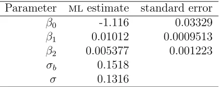
log(r′

ijkl) =β0+β1a′_p,i+β2f_j′ +bijk+εijkl (11)

The ml _{estimates of the parameters for the model in Equation (11) are}

406

displayed in Table 4. The corresponding AIC is -45.28, the maximum

log-407

Likelihood is 27.64 and npar = 5. 408

[Table 4 about here.]

409

5. Discussion

410

The fixed effects part of the model of Equation (8) and (9) allows predictions

411

to be made regarding the typical efficiency ratio ˆE [rijkl] when the technolog-412

ical variables are set within the experimental region investigated. Figure 6

413

provides an operational graphical representation of this model to assist its

414

interpretation.

415

[Figure 6 about here.]

416

In such a figure, the yellow or light-grey transparent area respectively in

417

colour and black-and-white print represents the region of the technological

418

parameters experimentally explored. For any dimensionless feed rate in that

419

area, increasing the cutting speed deteriorates the expected efficiencyr. The

420

maximum expected efficiency ratio in the area is 10.96 % and is obtained

at the minimum feed rate and minimum cutting speed investigated (point

422

A, at the corner of the yellow/light-grey region in Figure 6). The variable

423

v′

c enters the model with a coefficient that is approximately the double in 424

absolute value of that associated with f′ _{( ˆβ}

3/βˆ2 ∼= 2). This supports the 425

idea that the efficiency ratio r is more sensitive to per cent variations in

426

cutting speed rather than in feed rate. The positive interaction coefficient

427

( ˆβ6) is about one fifth of that of f′ and one tenth of that of v′_c (both taken 428

in absolute value). Hence for positive f′ _{the degree of sensitivity of the} 429

expected efficiency ratio r to v′

c is slightly less than what implied by ˆβ3 430

alone. In the experimental region investigated, however, this sensitivity to

431

v′

c is always larger than that to f′. When both f′ and vc′ are positive or 432

both are negative, the increment in efficiency ratio obtained by reducing

433

both f′ _{and v}′

c is less than the sum of the increments that can be obtained 434

by reducing f′ _{and v}′

c separately. The situation is reversed when f′ and 435

v′

c are of opposite sign. Any statement based on the extrapolation of the 436

model outside of the experimental region investigated needs per se further

437

experimental campaigns to be substantiated. However, an examination of

438

the behaviour of the model outside the region investigated experimentally

439

(the yellow/light-grey highlighted area in Figure 6) may assist the planning

440

of future experiments. In Figure 6, it is observed that when considering

441

f′ _{< −33.333 the sensitivity of the expected efficiency to the cutting speed} 442

is increased greatly. When instead 33.333 < f′ _{< 62.798, increments in} 443

cutting speed still decrease the efficiency, but less and less. The value ¯f′ ₌ 444

−βˆ3/βˆ6 = 62.798 is where any vc′ is expected to be equally efficient, namely 445

¯

r =eβˆ0− ˆ

β2βˆ3

ˆ

r is increasing and no longer descreasing with v′

c. The effect of vc′ on the 447

efficiency ratio is reversed because of the interation term in the model. The

448

point B in Figure 6 is the stationary saddle point of the model.

449

The above analysis indicates that in the investigated area and likely in large

450

areas beyond it (up to f′ _{<62.798), the cooling system is more efficient, the} 451

smaller the cutting speed and the feed rate are. Hence, the cooling system

452

is more efficient the smaller the mechanical power needed for the machining

453

operation is. A decrease in machining power is accompanied with a less than

454

proportional decrease in power dissipated by the cooling system.

455

Opposite to the case of the efficiency ratio r, the expected values of the

456

specific efficiency ratio r’ synthesised in Equation (11) do not exhibit any

457

dependence on the cutting speed v′

c. They do however display a dependence 458

on the depth of cut a′

p which does not exist for the ratio r. In contrast 459

with the ratio r, the log-transformed specific efficiency r’ does appear to be

460

linear in the significant independent variables. Otherwise stated, there is no

461

significant interaction between the two independent variables.

462

The model of Equation (11) shows that a unit volume flow rate of coolant

463

dissipates more thermal power out of the mechanical power needed to

gener-464

ate a unit volume flow rate of chip when the depth of cut and the feed rate

465

are larger. This conclusion seems consistent with the intuition that when

466

the contact tool-workpiece is larger the thermal exchange between workpiece

467

and tool is facilitated. Therefore more power can be dissipated into the tool

468

and then into the cooling system. Large depths of cut and large feed rates

469

increase the theoretical cross section of the chip (i.e. the cross section prior to

actual removal of the chip from the part). So therefore they do increase the

471

contact region tool-workpiece. The expected specific efficiency r’ is sensitive

472

to variations of depth of cut approximately twice as much it is to variations

473

of feed rate ( ˆβ1/βˆ2 ∼= 2). Whereas the depth of cut does not have any signif-474

icant effect on the efficiency r, increasing it appears to improve the specific

475

efficiency r’.

476

6. Conclusions

477

Microfluidic structures internal to the tool have been designed and

manufac-478

tured to convey the flow of coolant in the near proximity of the cutter edge.

479

The part and the coolant never enter in contact. Contamination of the part

480

by molecules of the coolant is thus prevented.

481

The designed and manufactured internally-cooled tool system enabled heat

482

transfer from the cutting zone of the insert to the flow of the liquid coolant.

483

Measurements of cutting force, thrust force, coolant temperature at the inlet

484

and at the outlet of the tool system were taken in a 33_{experimental conditions} 485

defined by the depth of cut, the feed rate and the cutting speed. Each

486

condition was replicated three times.

487

An efficiency ratior and a specific efficiency ratior’ were respectively defined

488

as the percentage of the whole machining power that is transferred to the

489

coolant and as the percentage of machining power per volumetric flow rate

490

of material removed that is transferred to a unit volume flow rate of the

491

coolant.

Linear mixed-effects statistical models were fitted to the experimental results

493

using the maximum likelihood method. The analysis revealed that the

effi-494

ciency ratio r depends exponentially on the cutting speed and on the feed

495

rate, whereas it does not depend on the depth of cut. Within the

investi-496

gated experimental region, the less the cutting speed and the feed rate are,

497

the higher the expected efficiency ratios r are. The maximum expected

effi-498

ciency is therefore obtained at fmin = 0.10 mm/rev and vc,min = 250 m/min 499

and is equal to 10.96 %. A significant interaction effect of cutting speed and

500

feed rate on the efficiency ratio r was also identified. The specific efficiency

501

ratio r’ was instead found exponentially depending on the depth of cut and

502

the feed rate with no significant interaction effect. In other words, the log(r′₎ 503

was found to be linearly increasing with the depth of cut and the feed rate.

504

Acknowledgements

505

This study is dedicated to the memory of Gualberto Ricci Curbastro for

506

no small amount of personal inspiration. The investigation was performed

507

within the scope of the collaborative research project ‘Self-learning control of

508

tool temperature in cutting processes’(ConTemp_{) funded by the European}

509

Commission 7th Framework Programme (Contract number:

NMP2-SL-2009-510

228585). The authors gratefully acknowledge the committed support of all

511

the technical staff in the AMEE Department at Brunel University. Particular

512

gratitude goes to Mr Paul Yates for his help in the cutting trials.

513

[1] V. P. Astakhov, The assessment of cutting tool wear, International

Jour-514

nal of Machine Tools and Manufacture 44 (6) (2004) 637 – 647.

[2] J. M. Longbottom, J. D. Lanham, Cutting temperature measurement

516

while machining a review, Aircraft Engineering and Aerospace

Tech-517

nology 77 (2005) 122–130.

518

[3] E. M. Trent, P. K. Wright, Chapter 5 - heat in metal cutting, in:

519

Metal Cutting (Fourth Edition), fourth edition Edition,

Butterworth-520

Heinemann, Woburn, 2000, pp. 97 – 131.

521

[4] Y. Quan, Z. He, Y. Dou, Cutting heat dissipation in high-speed

machin-522

ing of steel based on the calorimetric method, Frontiers of Mechanical

523

Engineering in China 3 (2) (2008) 175–179.

524

[5] A. Basti, T. Obikawa, J. Shinozuka, Tools with built-in thin film

thermo-525

couple sensors for monitoring cutting temperature, International Journal

526

of Machine Tools and Manufacture 47 (5) (2007) 793 – 798.

527

[6] G. Cohen, P. Gilles, S. Segonds, M. Mousseigne, P. Lagarrigue, Thermal

528

and mechanical modeling during dry turning operations, The

Interna-529

tional Journal of Advanced Manufacturing Technology 58 (1-4) (2012)

530

133–140.

531

[7] H. Young, T. Chou, Investigation of edge effect from the chip-back

tem-532

perature using IR thermographic techniques, Journal of Materials

Pro-533

cessing Technology 52 (24) (1995) 213 – 224.

534

[8] N. Jeffries, R. Zerkle, Thermal analysis of an internally-cooled

metal-535

cutting tool, International Journal of Machine Tool Design and Research

536

10 (3) (1970) 381 – 399.

[9] C. Ferri, T. Minton, S. Bin Che Ghani, K. Cheng, Internally-cooled tools

538

and cutting temperature in contamination-free machining, Proceedings

539

of the Institution of Mechanical Engineers, part C: Journal of

Mechani-540

cal Engineering Science(accepted for publication. OnlineFirst, 13 March

541

2013). doi:10.1177/0954406213480312.

542

[10] J. C. Rozzi, W. Chen, E. E. J. Archibald, Indirect cooling of a cutting

543

tool, USA Patent US 8,061,241 B2 (2011).

544

[11] L. E. A. Sanchez, V. L. Scalon, G. G. C. Abreu, Cleaner machining

545

through a toolholder with internal cooling, in: Proceedings of the 3rd

546

International Workshop Advances in cleaner production, Vol. 3, San

547

Paulo, 2011.

548

[12] L. Liang, Y. Quan, Z. Ke, Investigation of tool-chip interface

temper-549

ature in dry turning assisted by heat pipe cooling, The International

550

Journal of Advanced Manufacturing Technology 54 (1-4) (2011) 35–43.

551

[13] S. Shu, S. Chen, K. Cheng, Investigation of a novel green internal cooling

552

in turning application, in: Electronic and Mechanical Engineering and

553

Information Technology (EMEIT), 2011 International Conference on,

554

Vol. 3, 2011, pp. 1156–1159.

555

[14] E. Uhlmann, P. F¨urstmann, M. Roeder, S. Richarz, F. Sammler, Tool

556

wear beaviour of internally cooled tools at different cooling liquid

tem-557

peratures, in: Proceedings of the 10th _{Global Conference on Sustainable} 558

Manufacturing, Istanbul, Turkey, 2012.

[15] G. F. Micheletti, Tecnologia Meccanica - Il taglio dei metalli, Vol. 1,

560

UTET, 1977, (in Italian).

561

[16] G. Boothroyd, Temperatures in orthogonal metal cutting, Proceedings

562

of the Institution of Mechanical Engineers 177 (29) (1963) 789–810.

563

[17] E. M. Trent, P. K. Wright, Chapter 9 - machinability, in: Metal

Cut-564

ting (Fourth Edition), fourth edition Edition, Butterworth-Heinemann,

565

Woburn, 2000, pp. 251 – 310.

566

[18] J. Kopac, M. Sokovic, S. Dolinsek, Tribology of coated tools in

conven-567

tional and {HSC} machining, Journal of Materials Processing

Technol-568

ogy 118 (13) (2001) 377 – 384.

569

[19] E. M. Trent, P. K. Wright, Metal Cutting, 4th Edition,

Butterworth-570

Heinemann, Oxford, 2000.

571

[20] J. C. Pinheiro, D. M. Bates, Mixed-Effects Models in S and S-Plus,

572

Springer, 2000.

573

[21] J. Pinheiro, D. Bates, S. DebRoy, D. Sarkar, R Development Core Team,

574

nlme: Linear and Nonlinear Mixed Effects Models, r package version

575

3.1-103 (2012).

576

[22] R Development Core Team, R: A Language and Environment for

Sta-577

tistical Computing, R Foundation for Statistical Computing, Vienna,

578

Austria (2011).

579

[23] J. J. Faraway, Linear Models with R, 1st Edition, Texts in Statistical

580

Science, Chapman & Hall/CRC, 2004.

List of Figures

582

1 (a) The experimental set-up for the cutting trials. (b) A 3-D

583

model of the assembled internally cooled tool system. . . 29

584

2 The ratio r versus the dimensionless technological variables

585

a′

p, f′ and v′c. The abscissae have been jittered. The cross 586

designates the sample mean for each of the three groups of

587

data in each panel. . . 30

588

3 Residuals versus fitted values (alias predicted values) (a) of

589

the simplified model (Equation (7)) (b) of the log-transformed

590

simplified model (Equation 8 or 9). . . 31

591

4 The realisations of the non-observable residuals versus the

val-592

ues fitted by (a) the model that includes the random effects

593

(Equation 8) (b) the model that does not include the

ran-594

dom effects (Equation 10). The average for each treatment is

595

identified by the points ’X’. The shadow area underlying the

596

segments joining these averages facilitate the visualisation of

597

the different amount of violation of the assumed zero mean for

598

errors of the two models. . . 32

599

5 The ratio r’ versus the dimensionless technological variables

600

a′

p, f′ and v′c. The abscissae have been jittered. The cross 601

designates the sample mean for each of the three groups of

602

data in each panel. . . 33

603

6 The expected value of the efficiency ratio r versus the

di-604

mensionless cutting speed v′

c for selected f′ values ranging 605

from -100 to 100. The highlighted area in yellow/light-grey

606

in colour/black-and-white print represents the experimental

607

region investigated. The point A identifies the maximum

ef-608

ficiency in that area. The point B identifies the stationary

609

saddle point. The thicker dotted and dashed line is horizontal

610

(iso-efficient line). . . 34

−40 −20 0 20 40 4

6 8 10 12 14

a’p

r

−40 −20 0 20 40

4 6 8 10 12 14

f’ r

−20 −10 0 10 20

4 6 8 10 12 14

v’c

r

Figure 2: The ratio r versus the dimensionless technological variablesa′

p, f′ andvc′. The

(a) Fitted values, E~[r_{i j k}|b_{i j k}]

Residuals

,

ε

~ ijkl

−3 −2 −1 0 1 2

6 8 10 12

(b) Fitted values, E~[log(r_{i j k}) |b_{i j k}]

Residuals

,

ε

~ ijkl

−0.4 −0.2 0.0 0.2

1.6 1.8 2.0 2.2 2.4

66 a

66 c

(a) Residuals,

~

ε

Treatment

55 60 65 70 75 80

-0.4 -0.2 0.0 0.2

(b) Residuals,

~

ε

Treatment

55 60 65 70 75 80

-0.6 -0.4 -0.2 0.0 0.2 0.4

−40 −20 0 20 40 0.2

0.3 0.4 0.5 0.6 0.7 0.8

a’p

r’

−40 −20 0 20 40

0.2 0.3 0.4 0.5 0.6 0.7 0.8

f’ r’

−20 −10 0 10 20

0.2 0.3 0.4 0.5 0.6 0.7 0.8

v’c

r’

Figure 5: The ratior’ versus the dimensionless technological variablesa′

p,f′andv′c. The

Figure 6: The expected value of the efficiency ratiorversus the dimensionless cutting speed

v′

cfor selectedf

′_{values ranging from -100 to 100. The highlighted area in yellow/light-grey}

List of Tables

612

1 Technological variables and their values. . . 36

613

2 Sequential tests of the hypotheses for the significance of the

614

independent variables and their interactions both listed in the

615

first column. ‘numDF’ and ‘denDF’ are the numerator and

616

denominator degrees of freedom, respectively. The p-values

617

are expressed in fractions of the unity rather than in per cent. 37

618

3 ml_{estimates of the parameters for the model with Equation 8}

619

or 9. For the estimators of theβ’s the standard errors are also

620

shown. . . 38

621

4 ml _{estimates of the parameters for the model with}

Equa-622

tion 11. For the estimators of the β’s the standard errors

623

are also shown. . . 39

Table 1: Technological variables and their values.

Variable Unit values

depth of cut,ap mm 0.20, 0.35 and 0.50

feed rate, f mm/rev 0.10, 0.15 and 0.20

numDF denDF F-value p-value

(Intercept) 1 54 995.5 <0.0001

a′

p 1 19 0.01980 0.8896

f′ _{1 19 21.25 0.0002}

v′

c 1 19 25.99 0.0001

a′

pf′ 1 19 0.3581 0.5566

a′

pv′c 1 19 0.1678 0.6866

f′_v′

c 1 19 7.753 0.0118

a′

pf′v′c 1 19 2.1257 0.1612

Parameter ml_{estimate standard error}

β0 1.947 0.03105

β2 -0.005020 0.001141

β3 -0.01099 0.002282

β6 0.0001750 0.00008384

σb 0.1378

σ 0.1316

Parameter ml_{estimate standard error}

β0 -1.116 0.03329

β1 0.01012 0.0009513

β2 0.005377 0.001223

σb 0.1518

σ 0.1316