warwick.ac.uk/lib-publications
A Thesis Submitted for the Degree of PhD at the University of Warwick
Permanent WRAP URL:
http://wrap.warwick.ac.uk/93636
Copyright and reuse:
This thesis is made available online and is protected by original copyright.
Please scroll down to view the document itself.
Please refer to the repository record for this item for information to help you to cite it.
Our policy information is available from the repository home page.
in Multiple Sclerosis
by
Bernd Taschler
Thesis
Submitted to the University of Warwick for the degree of
Doctor of Philosophy
Centre for Complexity Science
Contents
List of Tables v
List of Figures vii
Acknowledgments ix
Declarations x
Abstract xi
Abbreviations xii
Chapter 1 Introduction 1
Chapter 2 Background 4
2.1 Neuroimaging: Magnetic Resonance Imaging . . . 4
2.1.1 Preprocessing steps . . . 6
2.2 Medical background: Multiple Sclerosis . . . 7
2.2.1 Disease pathology . . . 8
2.2.2 Diagnosis and MS subtypes . . . 9
2.2.3 Therapy . . . 11
2.2.4 MRI criteria . . . 12
2.2.5 Quantitative analysis . . . 13
2.3 Methodological background: Spatial point processes . . . 14
2.3.1 Spatial Poisson point processes . . . 15
2.3.2 The log-Gaussian Cox process . . . 17
2.3.3 Poisson/Gamma random fields . . . 18
2.3.4 Inverse L´evy measure construction of a Gamma random field 19 2.3.5 Data augmentation: Auxiliary points . . . 20
2.3.7 Multiple realisations . . . 22
2.3.8 Marked point processes . . . 24
2.4 Methodological background: Classification and prediction . . . 25
2.4.1 Cross-validation . . . 25
2.4.2 A Bayesian classifier for multi-type point patterns . . . 26
Chapter 3 Two clinical data sets 29 3.1 The GeneMSA data set . . . 29
3.2 The BENEFIT data set . . . 36
Chapter 4 Comparison of two machine learning approaches and two spatially informed models for MS subtype classification 40 4.1 Introduction . . . 40
4.2 A na¨ıve Bayesian classifier . . . 41
4.3 Support vector machines based on lesion-specific features . . . 42
4.3.1 Support Vector Machines . . . 42
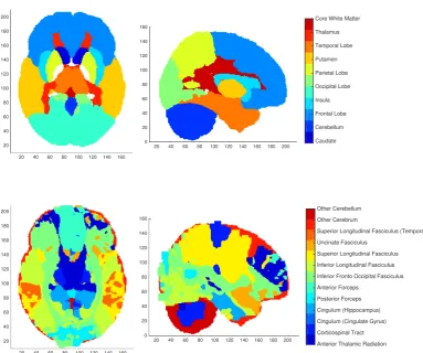
4.3.2 Minkowski functionals and lesion geometry . . . 46
4.3.3 The feature set . . . 47
4.3.4 Principal component analysis . . . 50
4.3.5 Model evaluation . . . 51
4.4 A Bayesian Spatial Generalised Linear Mixed Model . . . 52
4.5 A Bayesian log-Gaussian Cox process model . . . 53
4.6 Application: GeneMSA data . . . 55
4.6.1 SVM feature inference . . . 56
4.6.2 Posterior probability and intensity maps . . . 59
4.6.3 Prediction Accuracies . . . 62
4.7 Discussion . . . 66
Chapter 5 Poisson/Gamma random field models for spatial point data 68 5.1 Introduction . . . 68
5.2 The hierarchical PGRF model . . . 69
5.3 Including covariates . . . 71
5.3.1 Poisson regression . . . 72
5.4 Marked hierarchical PGRF models . . . 73
5.4.1 The marked HPGRF model with additional covariates . . . . 74
5.4.2 Assuming an independent mark distribution . . . 75
CONTENTS iii
5.4.4 Variance-stabilised marks . . . 77
5.5 Posterior approximation and sampling algorithm . . . 77
5.6 Simulation study . . . 78
5.6.1 Simulated spatial data . . . 79
5.6.2 Simulated covariates . . . 80
5.6.3 Simulated mark process . . . 80
5.6.4 Simulation setup . . . 81
5.6.5 Simulation results and model assessment . . . 82
5.7 Discussion . . . 94
5.7.1 Limitations . . . 95
5.7.2 Further extensions . . . 96
Chapter 6 Application of spatial point process models to MS lesion data 98 6.1 Application: GeneMSA data . . . 99
6.1.1 Algorithmic details and posterior computation . . . 99
6.1.2 Posterior results and prediction . . . 100
6.1.3 Model assessment . . . 108
6.1.4 A GLM analysis . . . 109
6.2 Application: BENEFIT data . . . 111
6.2.1 Algorithmic details and posterior computation . . . 111
6.2.2 Posterior results and prediction . . . 112
6.2.3 Model assessment . . . 116
6.2.4 A GLM analysis . . . 117
6.3 Discussion . . . 118
Chapter 7 Conclusions 122 7.1 Contributions . . . 122
7.2 Future work . . . 124
Appendix A imHPGRF supplements 126 A.1 Posterior computation . . . 126
A.1.1 Sampling of mark parameters . . . 127
A.1.2 Sampling of regression coefficients . . . 129
A.1.3 Sampling of Gamma random fields . . . 130
A.1.4 Sampling of kernel parameters . . . 135
Appendix B Application supplements 138
List of Tables
2.1 Summary of MS lesion types. . . 13
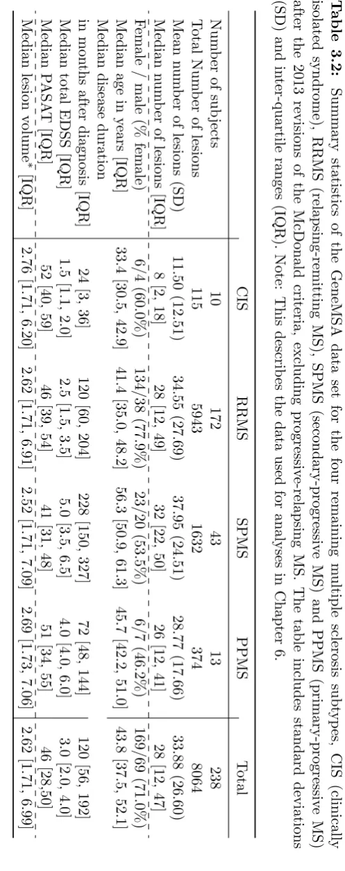
3.1 Summary statistics of the GeneMSA data set including the PRMS subtype. . . 33
3.2 Summary statistics of the GeneMSA data set excluding the PRMS subtype. . . 34
3.3 Summary statistics of the BENEFIT data set. . . 39
4.1 Summary of feature sets for the SVM classifier. . . 51
4.2 Parameter estimates for the LGCP model. . . 55
4.3 Confusion matrices and prediction accuracies for different classifiers (T1). . . 64
4.4 Confusion matrices and prediction accuracies for different classifiers (T2). . . 65
5.1 Parameter specification for simulated data sets. . . 79
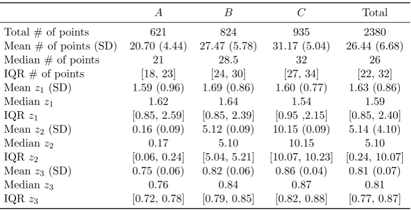
5.2 Summary statistics of simulated points and covariates. . . 80
5.3 Summary statistics of simulated mark values. . . 81
5.4 Mean posterior estimates of average count per group. . . 87
5.5 Summary of IMSE, IWMSE and mark residuals. . . 91
5.6 Ground truth and mean posterior estimates of mark parameters. . . 92
5.7 Ground truth and mean posterior estimates of regression coefficients. 92 5.8 Simulation study: Summary of confusion matrices and prediction ac-curacies. . . 93
6.1 GeneMSA results: Posterior parameter estimates of type-specific pa-rameters for the imHPGRF model including covariates. . . 103
6.3 GeneMSA results: Confusion matrices for different model variants. . 107 6.4 GeneMSA results: Posterior estimates of the average number of
le-sions per subject for each MS subtype. . . 109 6.5 GeneMSA results: Results from fitting a GLM to subject-specific
covariates. . . 110 6.6 BENEFIT results: Posterior parameter estimates of type-specific
pa-rameters for the imHPGRF model including covariates. . . 114 6.7 BENEFIT results: Posterior parameter estimates of shared
parame-ters for the imHPGRF model including covariates. . . 114 6.8 BENEFIT results: Confusion matrices for different model variants. . 116 6.9 BENEFIT results: Posterior estimates of the average number of
le-sions per subject. . . 117 6.10 BENEFIT results: Summary of results from fitting a GLM to
List of Figures
2.1 Example MRI of a standard brain template and MS lesions. . . 7
2.2 Schematic depiction of disease progression for the four clinical sub-types of multiple sclerosis. . . 11
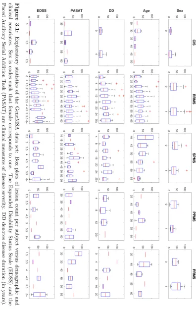
3.1 GeneMSA data set: Box plots of lesion count versus demographic and clinical covariates. . . 32
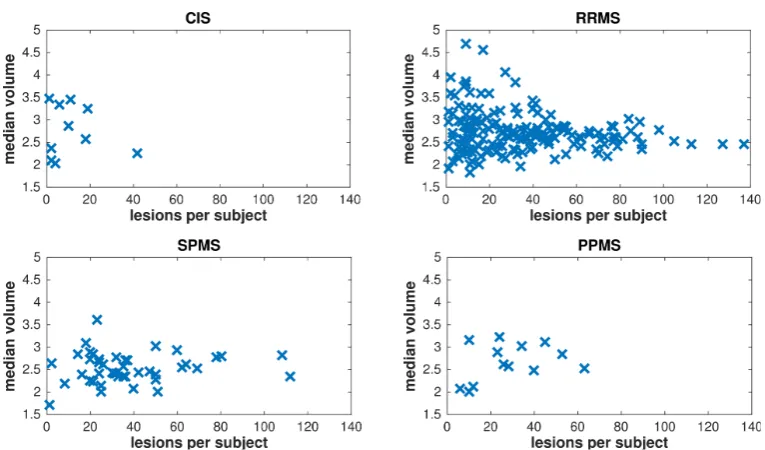
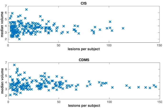
3.2 GeneMSA data set: Scatter plots of lesion volume versus lesion count. 35 3.3 BENEFIT data set: Scatter plots of lesion volume versus lesion count. 37 3.4 BENEFIT data set: Box plots of lesion count versus demographic and clinical covariates. . . 38
4.1 Visualistion of two brain segmentations into regions of interest. . . . 49
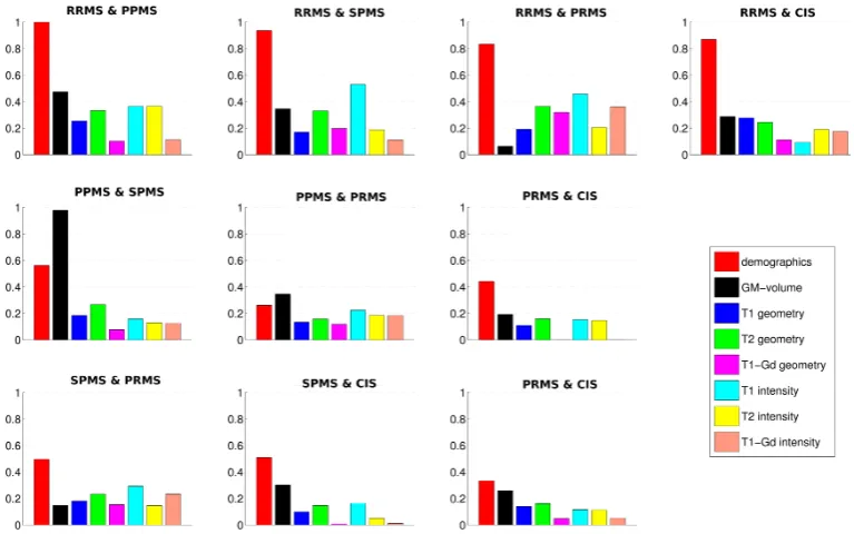
4.2 Standardised SVM weights for one pairwise classifier. . . 58
4.3 Quadratic means of SVM weights for pairwise classifiers. . . 59
4.4 Results for the BSGLMM and LGCP model fit (axial). . . 60
4.5 Results for the BSGLMM and LGCP model fit (sagittal). . . 61
4.6 Standardised coefficient maps of subject-level covariates for the BS-GLMM model fit. . . 62
5.1 Simulation study: Posterior traceplots of scalar model parameters. . 83
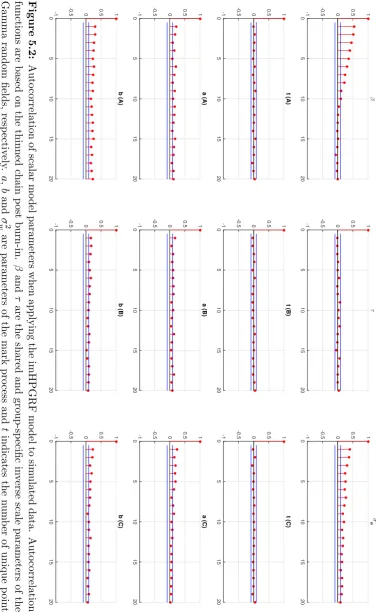
5.2 Simulation study: Autocorrelation of scalar model parameters. . . . 84
5.3 Simulation setup and estimated posterior mean spatial intensities. . 85
5.4 True and estimated posterior mean intensity of the simulated mark process. . . 86
5.5 Results of the posterior predictive check for second order properties of the point process. . . 88
5.6 Simulation study: Mark residuals versus predicted values. . . 89
6.1 GeneMSA results: Empirical and estimated posterior intensity maps
per MS subtype (axial). . . 101
6.2 GeneMSA results: Empirical and estimated posterior intensity maps per MS subtype (sagittal). . . 102
6.3 GeneMSA results: Mark residuals of posterior estimates of individual lesion volume. . . 104
6.4 GeneMSA results: Covariate residuals from Poisson regression of pos-terior estimates of lesion count. . . 104
6.5 GeneMSA results: GLM fit. . . 109
6.6 BENEFIT results: Estimated posterior intensity maps (axial). . . 112
6.7 BENEFIT results: Estimated posterior intensity maps (sagittal). . 113
6.8 BENEFIT results: Mark residuals of posterior estimates of individual lesion volume. . . 115
6.9 BENEFIT results: Covariate residuals of posterior estimates of lesion count per subject. . . 115
6.10 BENEFIT results: GLM fit. . . 118
B.1 Standardised SVM weights for five pairwise classifiers (I). . . 139
B.2 Standardised SVM weights for five pairwise classifiers (II). . . 140
B.3 GeneMSA results: Traceplots for parameters of the imHPGRF model. 142 B.4 GeneMSA results: Autocorrelation plots for parameters of the imH-PGF model . . . 143
B.5 GeneMSA results: Square-root transformed posterior mean intensity for MS subtype CIS. . . 144
B.6 GeneMSA results: Square-root transformed posterior mean intensity for MS subtype RRMS. . . 145
B.7 GeneMSA results: Square-root transformed posterior mean intensity for MS subtype SPMS. . . 146
B.8 GeneMSA results: Square-root transformed posterior mean intensity for MS subtype PPMS. . . 147
B.9 BENEFIT results: Traceplots for parameters of the imHPGRF model. 149 B.10 BENEFIT results: Autocorrelation plots for parameters of the imH-PGRF model. . . 150
B.11 BENEFIT results: Square-root transformed posterior mean intensity for CIS. . . 151
Acknowledgments
I would like to express my heartfelt gratitude and appreciation to my supervisor Tom Nichols. His excellent support and guidance, his ability to motivate, his deep interest in and knowledge of neuroimaging statistics, combined with lots of patience and a sense of humour have helped me in countless ways over the course of my Ph.D. and, ultimately, to become a better researcher.
I want to thank Tim Johnson for numerous interesting discussions and for sharing his wide-ranging insights of various areas of statistics.
I am especially grateful to Ernst-Wilhelm Rad¨u, Jens W¨urfel and the Medi-cal Image Analysis Center in Basel for financially supporting and thereby allowing me to carry out this work. I would like to thank Kerstin Bendfeldt for a great re-search collaboration and everybody at MIAC for their hospitality and the welcoming atmosphere every time I came to visit.
Many thanks are due to my dear friends and colleagues, especially Silvia and Pantelis and everybody else in Tom’s group. Our discussions whether about research or other matters are invaluable to me. The same holds true for my office mates Ellen, Ed, Fede, Joe and Illiana with whom I had the joy and privilege to share an office for several years. I want to thank everybody at the Centre for Complexity Science for creating and enabling such an interesting, supportive and joyful research environment.
Declarations
This thesis is submitted to the University of Warwick in support of my application for the degree of Doctor of Philosophy. It has been composed by myself and has not been submitted in any previous application for any degree. The work presented (including data generated and data analysis) was carried out by the author except in the cases outlined below:
• The GeneMSA and BENEFIT data sets used in Chapter 4 and Chapter 6 were provided by the Medical Image Analysis Center in Basel, Switzerland.
Abstract
Abbreviations
BSGLMM Bayesian spatial generalised linear mixed model CDMS clinically definite multiple sclerosis
CIS clinically isolated syndrome GM grey matter
HPGRF hierarchical Poisson/Gamma random field
imHPGRF intensity-marked hierarchical Poisson/Gamma random field LGCP log-Gaussian Cox process
MCMC Markov chain Monte Carlo MRI magnetic resonance imaging
MS multiple sclerosis
PGRF Poisson/Gamma random field
PPMS primary-progressive multiple sclerosis PRMS progressive-relapsing multiple sclerosis RRMS relapsing-remitting multiple sclerosis
SPMS secondary-progressive multiple sclerosis SVM support vector machine
ABBREVIATIONS
The facts of science, as they appeared to him [Heraclitus], fed the flame in
his soul, and in its light, he saw into the depths of the world by the
reflection of his own dancing swiftly penetrating fire.
—Bertrand Russell,Mysticism and Logic (1918)
I am a brain, Watson. The rest of me is a mere appendix. Therefore, it is the brain I must consider.
Introduction
low predictive value and therefore are poor indicators for determining the clinical outcomes in MS [Loevblad et al., 2010].
Existing quantitative methods that are commonly used for the analysis of MS lesions are, to a large extend, unable to exploit the richness of the imaging data. A prominent method is based on the analysis of lesion probability masks that are compared either cross-sectionally or longitudinally [Filli et al., 2012; Holland et al., 2012] which makes it difficult to associate lesion locations with certain covariates of interest. Furthermore, mass-univariate methods such as voxel-based lesion-symptom mapping [Bates et al., 2003] are ill suited for the binary nature of lesion data and cannot account for the underlying spatial structure. Finally, smoothing kernels are commonly used to introduce a degree of spatial correlation in the data. However, the smoothing of lesion masks by means of a Gaussian kernel [Kincses et al., 2011] does not entirely eliminate the non-Gaussian nature of the data and requires an arbitrary choice of smoothing parameter.
Motivated by these challenges, this thesis explores ways of increasing the utilisation of available imaging data by combining quantitative measures derived from MRI with clinical information. A particular focus of this work lies in the use of statistical methods that rely upon or at least are informed by spatial data. We are interested in the analysis of spatial point patterns that are a result of MRI data and propose a Bayesian spatial point process approach that uses locations of individual lesions to model point pattern data. We are drawn to the Bayesian approach due to the very sparse, high-dimensional nature of the neuroimaging data. Bayesian meth-ods also have the advantage of being able to incorporate prior knowledge, reducing the complexity of the analysis and offering greater precision when sample sizes are low.
This work offers several novel contributions. We make a direct comparison of point process and machine learning methods for predicting disease subtype, finding the point process model has superior performance even when based on much less rich data. We extend the hierarchical Poisson/Gamma random field model to allow for covariates and marks. We develop all of this work in the setting of three-dimensional, multiple-class, multiple-realisation point process data, conduct thorough evaluations on simulated data and apply the methods on two real datasets.
convolution of a kernel with a Gamma random field, in particular. The chapter continues with a brief discussion of classification and prediction procedures with respect to cross-validation and concludes with the presentation of two clinical data sets that form the basis for the application of our models.
Chapter 4 concentrates on four different approaches to classification and prediction of MS lesion data. The four models include a na¨ıve Bayesian classifier, a support vector machine approach based on a large feature set that encompasses clinical as well as imaging data with a focus on geometric measures of individual lesions, a Bayesian spatial generalised linear mixed model that relies on a probit regression framework and, finally, a log-Gaussian Cox process model fitted to the coordinates of the centres–of–mass of individual lesions.
Our main spatial point process model is a Poisson/Gamma random field model that builds upon the work by Wolpert and Ickstadt [1998b] and Kang et al. [2014a] and is presented in Chapter 5. In particular, we outline a hierarchical for-mulation of the model that allows for the sharing of information between distinct but related point processes, and then propose ways of extending the model. First, we introduce external covariates, which are specific to a given realisation of a point pattern. A second extension combines the spatial point process model with an addi-tional mark process that carries location-specific attributes of each observed point. We further apply and compare different model variants in a simulation study.
Chapter 2
Background
In this chapter we lay out the background material relevant to the subsequent chap-ters of the thesis. Section 2.1 covers the technical details of magnetic resonance imaging, including image acquisition and processing methods. Section 2.2 provides medical background on multiple sclerosis. Section 2.3 summarises the statistical methodology underlying the spatial point process models and methods presented later on in Chapter 5. In Section 2.4 we review some aspects of classification in-cluding cross-validation and introduce a Bayesian importance sampling algorithm. Finally, Chapter 3 introduces the two MS data sets that are the basis for model applications in Chapter 4 and Chapter 6.
2.1
Neuroimaging: Magnetic Resonance Imaging
In magnetic resonance imaging (MRI) of the brain, a broad distinction is made between functional and structural MRI. Functional MRI (fMRI) is used as a physio-logical measure that tracks rapidly changing oxygen levels in the brain’s blood flow. The technique is widely used to investigate neural activity in response to various tasks. On the other hand, structural MRI (sMRI) is used to visualise details of the anatomy which are unchanging on a short time scale. Due to the necessity of capturing the brain’s activity within a limited time frame, the acquisition time of fMRI is significantly shorter resulting in a lack of spatial resolution compared to structural images.
researchers have investigated the brain’s activity when being in love [Ortigue et al., 2010], while composing music [Lu et al., 2015] or reading a suspense-novel [Lehne et al., 2015] or simply while being at rest [Cole et al., 2010; Lee et al., 2013]. However, structural MRI is the mainstay in clinical settings. It has become an important tool to detect and visualise abnormalities in the physical appearance of the brain and to track changes over time. Structural MRI is highly effective at identifying lesions and therefore is widely used in the diagnosis and assessment of diseases like multiple sclerosis, Alzheimer’s, epilepsy and schizophrenia.
MRI is by no account the only imaging technique that is currently used in a clinical context, but for neurological disorders it is often the modality of choice. Other procedures used include (i) Computed Tomography (CT) [Bar-Shalom et al., 2003] which has fine spatial resolution but utilises x-rays and therefore has the inherent disadvantage of exposure to ionising radiation. (ii) Positron Emission To-mography (PET) [Alauddin, 2012], which uses gamma rays emitted by an injected radioactive tracer, can have exquisite biological specificity but has relatively poor spatial resolution and, of course, also entails exposure to ionising radiation. (iii) Electroencephalography (EEG) measures electric currents on the surface of the scalp which are a result of coherent electrical activity in the brain; EEG has good tempo-ral, but poor spatial resolution which limits its usefulness for clinical applications. (iv) Magnetoencephalography (MEG) is similar to EEG but captures magnetic fields emitted by the brain’s electrical activity [Sakkalis, 2011]. (v) Less wide-spread tech-niques include Near-Infrared Spectroscopy (NISR) which uses light to detect alter-ations in the concentration of oxygenated and de-oxygenated haemoglobin [Murkin and Arango, 2009], and Nuclear Magnetic Resonance (NMR) spectroscopy [Neema et al., 2007].
Magnetic resonance imaging manipulates the alignment and subsequent re-laxation of nuclear spins using a strong pulsed external magnetic field. There are two basic types of imaging sequences that each reflect different relaxation properties of the examined tissue after the nuclear spins have been aligned as a result of the external magnetic field: T1-weighted MRI uses the spin-lattice relaxation time after
which the longitudinal component of the nuclear spins have fully returned to their equilibrium orientation. The repetition time (TR) between consecutive pulses of the external magnetic field must be short in order to achieve T1 weighting.
Differ-ent tissues exhibit differDiffer-ent relaxation times. Most importantly, the T1 relaxation
time for water (mainly protons) is about five times larger than for fatty tissue. In contrast, T2-weighted scans exploit the spin-spin relaxation time, i.e. the time it
This is achieved by using a long echo time (TE), that is the time between the radio-frequency pulse and the echo signal, in the scanning protocol. A full review of the physical principles of magnetic resonance imaging is beyond the scope of this the-sis. An introductory treatment of the basics of MR physics can be found in Pooley [2005]. For an excellent, detailed review, see for example Currie et al. [2013].
In addition to traditional MRI scans, a standard procedure for MS patients involves the use of a contrast agent, such as Gadolinium, to improve the contrast between lesions and normal brain tissue. Gadolinium is used in combination with T1-weighted MRI to enhance visibility of acute inflammation which is associated
with breaches in the blood-brain-barrier [Filippi et al., 1996].
2.1.1 Preprocessing steps
After acquisition of an MRI scan, the data needs to be processed in order to be used for any statistical analysis, especially when multiple scans and/or multiple subjects are involved in the study. Several steps are commonly used to reduce artefacts, align and standardise the data. Due to the fact that, in most acquisition types, the full MRI is acquired slice-by-slice, time-dependent signals such as BOLD (blood-oxygen-level dependent) contrast imaging, require slice timing corrections. This is a standard preprocessing step for fMRI data, for example.
Spatial realignment is necessary to correct for head motion during a serial image acquisition like fMRI and typically involves a rigid body transformation of the whole image. Furthermore, spatial co-registration to a specific subject or equiv-alently spatial normalisation to a common brain template is needed in order to align data from multiple subjects who naturally differ in brain size and shape [Fris-ton et al., 2007]. A standard target space for spatial normalisation is provided in form of the atlas of the Montreal Neurological Institute (MNI). Additionally, spatial smoothing of the data with a Gaussian kernel is often used in an attempt to correct still existing misalignments after spatial normalisation. Smoothing decreases the spatial resolution but can increase the signal-to-noise ratio and the Gaussianity of the data.
Figure 2.1: Left panel: Example MRI of a standard brain template, showing coro-nal (upper left), sagittal (upper right) and axial (bottom left) views. The crosshairs indicate the origin in MNI space. Right panel: Example MRI of an MS patient with and without colouring of lesions on a T2-weighted scan. The subject shown is part
of the GeneMSA data set.
2.2
Medical background: Multiple Sclerosis
Neuroanatomy distinguishes between three main physiological components of the brain: white matter (WM), grey matter (GM) and cerebro-spinal fluid (CSF). White matter consists of myelinated axons and forms the connections between various areas of the brain. Its main function is to transmit electrical impulses. On the other hand, GM consists predominantly of neuronal cell bodies and unmyelinated neurons and makes up most of the cortical structure where brain functions such as sensory and motor areas are located. The CSF plays a role in protecting the brain from concussions as well as in regulating the cerebral blood flow. A typical neuron is composed of a cell body (soma), dendrites which act as receiver of electrical signals from other neurons and an axon which transmits impulses from the cell body to other areas of the brain. Axons are also called nerve fibres and are surrounded by a myelin (a kind of lipid) sheath.
neuronal conductivity which can take the form of temporal, acute inflammation or chronic tissue damage. Depending on which nerves are affected the symptoms vary considerably from patient to patient, including loss of vision, deprivation of motor and sensory functions, fatigue, cognitive impairment, digestive and sexual dysfunction, mood disorders and chronic pain; for a detailed medical description of MS see for example [Cohen and Rae-Grant, 2010].
2.2.1 Disease pathology
The course of the disease is characterised by episodes of acute relapses where the disease shows high activity and periods of remission during which patients present no or significantly weaker clinical symptoms. In later stages, disease pathology usually takes on a progressive form with increasing severity of symptoms and permanent disability after ten to fifteen years [Cohen and Rae-Grant, 2010].
In general, lesions can be found throughout the brain with a higher dispo-sition in white matter regions around the ventricles. A typical example of lesions found on magnetic resonance imaging are shown in Figure 2.1. Recent studies have also stressed the importance of demyelination and brain atrophy in grey matter [Bendfeldt et al., 2012]. Lesions tend to have an ovoid configuration and in early stages of the disease the lesions are typically thin and elongated.
The pathogenesis of MS is only partially understood. There is no clinical consensus as to what causes the disease. Both T cell and B cell mechanisms1 have been implicated as well as genetics (e.g. people of Northern European descent ap-pear to be at higher risk [Goldenberg, 2012]) and environmental factors [Compston and Coles, 2008]. However, a recent meta-analysis by Belbasis et al. [2015] has shown that many studies relating MS to environmental risk factors may be incon-clusive or even invalid, finding evidence only for the following factors: a biomarker of the Epstein-Barr virus, infectious mononucleosis and smoking. Furthermore, patho-genesis also differs significantly between individuals [Morales et al., 2006]. One of the few common aspects across patients is that early stages of the disease are in most cases characterised by acute inflammatory activity, whereas permanent neuro-degeneration is dominant in late and purely progressive MS [Cohen and Rae-Grant, 2010] with symptoms mainly due to axonal loss [Ge, 2006].
Disease burden is often quantified in terms of lesion load, which indicates the total lesion volume or number of lesions. A more general quantitative measure is
1B lymphocytes and T lymphocytes are types of white blood cells. T cells can be distinguished
brain atrophy, which is considered to describe the net accumulative disease burden as the consequence of all types of pathological processes found in the brain. Further-more, women are more often affected by the disease with a predominance of about 3:2 over male patients [Cohen and Rae-Grant, 2010].
2.2.2 Diagnosis and MS subtypes
First diagnostic criteria for multiple sclerosis were introduced by Schumacher et al. [1965] and two decades later refined by Poser et al. [1983]. The most comprehensive clinical criteria were introduced by McDonald et al. [2001] and are still called the “McDonald criteria”. These guidelines set the standard for the diagnosis of MS. According to the McDonald criteria, patients were grouped into five distinct clinical categories (phenotypes) depending on disease progression, which differs significantly between these subtypes of MS. The subtypes are: relapsing-remitting MS (RRMS), primary-progressive MS (PPMS), secondary-progressive MS (SPMS), progressive-relapsing MS (PRMS) and clinically isolated syndrome (CIS). The McDonald criteria have been updated in 2005 [Polman et al., 2005] and again in 2010 [Polman et al., 2011] to provide better measures of dissemination of lesions in time.
The McDonald criteria are designed for use by a practising physician. The most current revision of the criteria occurred in 2013 and was published by [Lublin et al., 2014]. One of the most important outcomes of the revised guidelines was that PRMS, which affected about 5% of MS patients, was dropped as a distinct clinical category. It was used to describe a disease course that is characterised by regular relapses and a steady progression in symptom severity starting already at disease onset. Additionally, the authors of the revised criteria have put a stronger emphasis on disease activity, measured by clinical relapse rate and MRI findings as well as disease progression, in their recommendations of clinical assessment of MS.
How-ever, a relapse may never completely revert to normal and many patients are left with a residual disability.
Secondary-progressive MS (SPMS) exhibits relapses as well, however, remis-sion occurs only partially and the severity of symptoms increases gradually over time. SPMS is most typically seen 10–15 years after the onset of RRMS [Cohen and Rae-Grant, 2010], with 90% of patients initially diagnosed with RRMS eventually developing into SPMS within 25 years [Ebers, 2001]. There is no distinct transition between the two forms of MS. The relapse rate tends to decrease in SPMS with additional incremental progression between relapses. Furthermore, lesion load tends to be higher in SPMS than in RRMS [Rovaris et al., 2006].
The last disease subtype encompasses clinically isolated syndromes (CIS). In the absent of any prior diagnoses and clinical symptoms, the first acute attack is referred to as a clinically isolated syndrome [Hurwitz, 2009]. The neurological episode is a sign of acute inflammation and must be consistent with demyelination in the central nervous system to be categorised as CIS [Freedman et al., 2014]. Patients with CIS may or may not subsequently develop one of the other courses of MS. In the 2013 revisions of the McDonald criteria, CIS has been recognised as the first clinical presentation of a disease that could be MS. For it to be diagnosed as clinically definite MS (CDMS), dissemination of demyelinating events in time must also occur [Lublin et al., 2014]. A schematic comparison of disease progression for different subtypes is given in Figure 2.2.
In addition, the 2014 guidelines for the first time included the category of ra-diologically isolated syndrome (RIS). It describes the case where the patient presents no clinical signs or symptoms but incidental imaging findings suggest inflammatory demyelination. RIS is not considered an MS subtype per se since clinical evidence of a demyelinating disease, which is a key criterion in current MS diagnosis, is absent. However, based on location and morphology of lesions as detected on MRI, RIS may suggest the presence of MS [Lublin et al., 2014].
Figure 2.2: Schematic depiction of disease progression for the four clinical subtypes of multiple sclerosis. Left panel: Relapsing-remitting MS (RRMS) and secondary-progressive MS (SPMS). Note that the transition from RRMS to SPMS is fluid and occurs typically 10 to 15 years after disease onset. Right panel: Clinically isolated syndrome (CIS), primary-progressive MS (PPMS) and progressive-relapsing MS (PRMS). PRMS was dropped in the 2013 revisions of the McDonald criteria. (Figure adapted from Cohen and Rae-Grant [2010]).
several sub-categories that are associated with various functional systems, such as visual (VSLSC), sensory (SENSSC), mental (MNSC), pyramidal (PYRSC, measures the ability to walk), cerebellar (CRBLSC, coordination), brain stem (BRSTMSC), and bowel and bladder (BWLSC) functions.
The paced auditory serial addition task (PASAT) [Gronwall, 1977] is a cog-nitive test, where a lower score indicates more severe impairment. It measures pro-cessing speed, working memory and arithmetic ability. PASAT is reasonably reliable but limited in scope and not specific to MS. New measures have been proposed, in-cluding, for example, patient-reported outcomes or biomarker measurements [Cohen et al., 2012].
2.2.3 Therapy
Fingolimod, Teriflunomide, Dimethyl fumarate, and Alemtuzumab as well as a con-siderable range of off-label treatment options. All approved agents try to reduce acute inflammation and appear to be more effective in early stages of the disease [Torkildsen et al., 2016]. Therapy, when effective, is able to prolong the time to subsequent attacks, reduce inflammation and formation of new lesions, and can help to slow disability progression and cognitive impairment.
2.2.4 MRI criteria
Neuronal damage develops into lesions which can then be seen on magnetic res-onance imaging. Although MRI is the main source of quantitative data for the diagnosis of MS, the correlation between lesions and clinical symptoms is only de-scribed as approximate. The reason for this may lie in neural plasticity and repair mechanisms that can compensate for damage. Therefore, MRI scans may not fully reflect functional changes in affected areas [Cohen and Rae-Grant, 2010].
Conventional MRI sequences that show different aspects of disease activ-ity and for which MRI criteria have been developed include T2-weighted and T2
-weighted fluid-attenuated inversion recovery (FLAIR) images, as well as T1-weighted
scans, both with and without the addition of a contrast agent such as Gadolin-ium (Gd). T1-weighted sequences display chronic or persistent hypo-intense lesions.
These so-called “black holes” indicate permanent axonal loss and neuronal damage. However, studies about the correlation of black holes and disability have been con-tradictory and the relationship with relapse rates is similarly inconsistent [Sahraian et al., 2010]. In Gd-enhanced T1 images, the contrast agent Gadolinium is used
to augment the appearance of inflammatory lesions. Gd-enhanced images show breaches of the blood-brain barrier that accompany acute MS attacks, for example during a relapse, revealing regions where the disease is presently active. Finally, T2-weighted scans are used to assess the cumulative disease burden, i.e. total lesion
load. Lesions appear hyper-intense on T2-weighted images. These sequences are also
used to detect the formation of new lesions. However, T2-weighted sequences lack
specificity as several other mechanisms such as edema, inflammation and gliosis (an increase in the number of a certain kind of neuroglial cell) add to the development of T2 lesions [Sahraian et al., 2010]. A summary of the different types of MS lesions
is provided in Table 2.1.
Table 2.1: Summary of MS lesion types. Type Appearance on MRI Characteristics
T1 hypo-intense (dark) chronic, persistent “black holes”,
indication of permanent neuronal damage T2 hyper-intense (bright) used for assessment of total lesion burden
T1-Gd contrast enhanced (bright) “active” lesions, indication of acute
inflammation
data is to a large extent only used in a qualitative way, assessing existence and gen-eral dissemination of lesions in space and time. For example, the diagnostic standard merely states that the presence of lesions in at least two of the typical anatomical regions (periventricular, juxtacortical, infratentorial areas) of the central nervous system or spinal cord is evidence for MS. The most common quantitative measure is lesion load, i.e. the total lesion volume. Previous work on using lesion load for classi-fication have been equivocal [Aban et al., 2008; Morgan et al., 2010; MacKay Altman et al., 2011]. Other studies have shown that conventional MRI measures have rather low predictive value and are therefore poor indicators for determining the clinical outcomes in MS [Loevblad et al., 2010]. There exists a need for quantitative MRI measures, for example to better understand the transition from RRMS to SPMS [Rovaris et al., 2006], and a more quantitative analysis of the data contained in and available through magnetic resonance imaging.
2.2.5 Quantitative analysis
Existing quantitative methods that are commonly used for the analysis of MS lesions are to a large extend unable to reflect the full complexity of the data. These include i) comparing lesion probability masks cross-sectionally or longitudinally [Filli et al., 2012; Holland et al., 2012] which makes it difficult to associate lesion locations with certain covariates of interest, ii) mass-univariate methods such as voxel-based lesion-symptom mapping [Bates et al., 2003] which cannot account for the underlying spatial structure, and iii) smoothing of lesion masks by means of a Gaussian kernel, see e.g. [Kincses et al., 2011], which does not entirely eliminate the non-Gaussian nature of the data and requires an arbitrary choice of smoothing parameter.
2.3
Methodological background: Spatial point processes
This section aims to provide some of the methodological background for the models presented in Chapter 5.
Statistical methodology for point pattern data advanced rapidly in the second half of the 20th century. One-dimensional non-homogeneous Poisson processes have been used to model, for example, geomagnetic reversal data, the occurrence of coal-mining disasters and arrivals at an intensive care unit (e.g. Lewis and Shedler [1979] and references therein). Ongoing research and applications can be found across many disciplines, including ecology and forestry [Ickstadt and Wolpert, 1999; Best et al., 2000, 2002; Stoyan and Penttinen, 2000; Niemi and Fern´andez, 2010; Woodard et al., 2010], geology, astronomy, material sciences and epidemiology [Vel´azquez et al., 2016]. Research interests focus on diverse topics such as the distributions of plant species [Illian et al., 2013; Renner et al., 2015], the occurrence of earthquakes over a certain period of time [van Lieshout and Stein, 2012], and astronomical data such as the distribution of stars or galaxies [Babu and Feigelson, 1996; Stoica, 2010]. Most of these example applications rely on summary statistics to analyse point patterns. See the extensive literature on summary statistics for point process applications, for example, Baddeley et al. [2000]; Gabriel and Diggle [2009]; Cronie and Van Lieshout [2015]; Cronie and van Lieshout [2016]. However, our focus of interest lies on estimating an underlying intensity function that is able to fully describe the generation of observed point patterns.
In the following, we give a short overview of key concepts and topics relating to the theory of spatial point processes with a particular emphasis on a Bayesian point of view. The main source for this is Møller and Waagepetersen [2004]. Most of the following material is covered in much greater detail in Daley and Vere-Jones [2003]; Daley and Vere-Jones [2008]; Illian et al. [2008]; Møller and Waagepetersen [2007]; Gelfand et al. [2010] and Diggle [2014].
A spatial point process Y is a random countable set of points {yi}∞i=1 in a
space S. We only consider Euclidean space here, i.e. S ⊆Rd. Typically, the region
of interest for realisations of the point process will be a bounded subset B ⊂ S, for example square kilometre of forest, a geographical region defined by political or natural boundaries, or a section of the night sky. For our purposes, d=3 and B
Let A be a bounded Borel set and let NY(A) denote the number of points
that fall intoA. NY(A) is the counting measure, i.e. a finite integer-valued measure, on A. Let y denote a single realisation of Y consisting of point locations yi. We
require that y is a locally finite subset of B, that is the cardinality n(·) of the set
{y∩A} is finite. The space of locally finite point configurations Nlf provides the
range ofY, i.e.
Nlf ={y⊆ B:n(y∩A)<∞}, ∀ A⊆ B. (2.1)
There are three distinct but equivalent ways to fully characterise a spatial point process: by its void probabilities (only for simple processes), its finite dimen-sional distributions and its generating functional.
The finite dimensional distributions are the joint distribution of the number of points ofY belonging to bounded Borel setsA1, . . . , Ak, such that
P[NY(A1) =n1;. . .;NY(Ak) =nk], n1, . . . , nk ∈N0. (2.2)
The void probabilities are defined as v(A) = P[NY(A) = 0] and the generating
functional for a point process is akin to a probability generating function for a non-negative, integer-valued random variable and is defined as
GY(u) =E
exp
Z
S
lnu(ξ)dN(ξ)
=E
Y
ξ∈y
u(ξ)
, (2.3)
where u is a function from S to [0,1] and ξ is a point in S such that u(ξ) ≤ 1. Consider as an exampleu(ξ) =tI[ξ∈A]with 0≤t≤1, then the probability generating
functional forNY(A) is GY(u) =E[tNY(A)].
2.3.1 Spatial Poisson point processes
Poisson point processes are making up the foundations of spatial point process the-ory. In their simplest variant they describe a random spatial point pattern with no correlation or any kind of interaction between points. Their defining property is that the number of points in any given region is a Poisson distributed random variable. Additionally, given the number of pointsNY(A) that belong to the process Y and
are contained in regionA⊆ B, those points are distributed independently according to a probability density that is proportional to an intensity function λ over that region.
an intensity measure Λ(A) = R
Aλ(ξ)dξ that is locally finite, i.e. Λ(A) <∞ for all
boundedA⊆ S and diffuse, i.e. Λ(ξ) = 0, for all pointsξ∈ S. A point processYon
S ⊆Rdis a Poisson point process with intensity functionλand intensity measure Λ
if the following to properties hold: (i) For anyA⊆Ssuch that Λ(A) is finite,NY(A)
is Poisson distributed with mean Λ(A). We writeNY(A)∼Pois(Λ(A)). (ii) For any disjointA1, . . . , Ak⊆ S, withk≥2, the random variablesNY(A1), . . . , NY(Ak) are
independent. If for a Poisson processY it holds that Λ(A) =
Z
A
λ(ξ)dξ (2.4) with Λ(A) < ∞ for any bounded A ⊆ S and λ some non-negative function on S, then we call Y a Poisson process with intensity function λ. The intensity is the first-order moment measure and also called the rate function. Analogously, Λ is sometimes called the integrated rate function. We denoteY ∼ PP(S, λ).
If the intensity function is constant (λ(ξ) =λ, for all ξ ∈ S), Y is called a
homogeneous orstationary process with rate λ. The special case of Y ∼ PP(S,1)
is called the standard or unit rate Poisson process. The void probabilities for a Poisson process are v(A) = exp{−Λ(A)} and the probability generating functional is given byGY(u) = exp{(1−u(ξ))λ(ξ)dξ}. The density (i.e. the Radon-Nikodym
derivative) of the Poisson process with respect to Lebesgue measure does not exist, but it does exist with respect to the unit rate Poisson processPP(B,1) [Møller and Waagepetersen, 2004]. The density is given by
π(y|λ) = exp
|B| −
Z
B
λ(ξ)dξ
Y
y∈y
λ(y), (2.5)
which can be interpreted as the density of the sampling distribution of the data. For most practical applications, a simple Poisson process is not sufficient to describe the observed point patterns. The class of Cox processes is a natural extension to the Poisson process. First introduced by Cox [1955], Cox processes are also called doubly stochastic processes, relating to the way the intensity function is modelled. Whereas the original Poisson process is based on a fixed parametric intensity, in the case of a Cox process, the intensity function is expressed as the realisation of a random variable or a random field.
Hence, letZ(ξ) be a non-negative random field onSsuch thatZ(ξ) is locally finite and integrable. IfY|Z ∼Pois(S, Z), thenYis said to be a Cox process driven by Z. The intensity function is simply the expectation over the random field, i.e.
will denote [Y|Λ]∼ PP(S,Λ) as being a spatial Poisson process driven by random intensity measure Λ [Møller et al., 1998]. Note that for disjoint boundedA1, A2 ⊂ S, NY(A1) andNY(A2) are positively correlated.
Cox processes have the advantage of allowing greater flexibility than, e.g. a parametric inhomogeneous Poisson process, and are better suited to model aggre-gated point patterns. Additionally, one can incorporate prior knowledge into the intensity function by using a Bayesian framework.
2.3.2 The log-Gaussian Cox process
One of the most commonly used Cox process models is the log-Gaussian Cox process (LGCP) [Møller et al., 1998], where the intensity function is a realisation of a random field Z. Assume that Z = lnλ is a Gaussian random field, that is a random pro-cess whose finite dimensional distributions are Gaussian; henceZ ∼ GP[m(·), c(·,·)] [Rasmussen and Williams, 2006]. The distribution of (Y, Z) is completely deter-mined by the mean and covariance function, which are given bym(r) =E[Z(r)] and c(r, s) =Cov[Z(r), Z(s)], respectively. The intensity function of the LGCP is given
by
λ(r) = exp [m(r) +c(r, r)/2], (2.6) where, for our later applications, we will assume that c(r, s) is isotropic and trans-lation invariant with the formc(r, s) =σ2exp−ρ||r−s||δ. The exponential term represents the power correlation function andδ ∈[0,2], which for δ=1 gives an ex-ponential and forδ=2 a Gaussian correlation; σ2 denotes the variance andρ>0 is a correlation parameter.
1998], which uses the gradient of the target distribution to guide a random walk update, to INLA.
2.3.3 Poisson/Gamma random fields
First introduced by Wolpert and Ickstadt [1998b], the Poisson/Gamma random field (PGRF) model was extended by Kang et al. [2014b] to incorporate multiple groups of related point patterns as well as multiple realisations of the underlying stochastic point process.
The fundamental characteristic of the PGRF model is that the intensity function is modelled as a convolution of a spatial kernel and a Gamma random field. In this section we will describe the main building blocks of the model. First, we recount the probability density of the Gamma distribution:
h(x;α, β) = β
α
Γ(α)x
α−1e−βx= 1
Γ(α)
α µ
α
xα−1exp
−αxµ
, (2.7) with x≥0 and α, β >0. Mean and variance of the Gamma distribution are given by
µ= α
β, σ
2 = α
β2 = µ2
α. (2.8)
A Gamma random field Γ(dx) has an inhomogeneous Gamma process distri-bution, i.e. Γ(dx)∼Ga{α(dx), β(x)}with shape measure (also called base measure)
α(dx) and inverse scale function (or rate parameter) β(x) > 0. For Γ(dx) to be a Gamma random field the following properties must hold: (i) for some setBand any partition {Ak} such that B =∪kAk, the random variables Γ(Ak) follow a Gamma
distribution with shape parameter α(Ak) = R
Akα(x)dx and mean α(Ak)/β(x) for
any x ∈Ak; (ii) for disjoint sets Ak∩Al =∅,k6=l, the Gamma random variables
Γ(Ak) and Γ(Al) are mutually independent. Note that the shape measure is
pro-portional to the volume and a convenient choice may be to use Lebesgue measure. For the rest of this thesis we take the inverse scale parameter β(x) to be constant over space and thus assumeβ(x)≡β.
The Gamma random field can be seen as a set of indicator functions with assigned Gamma distributed random variables. Realisations of Gamma random fields are discrete and consist of a countably infinite number of point masses, so-called jumps. Each jump location θm,m = 1, . . . ,∞, has an associated magnitude
(or jump height) ηm. Then, Γ(A) is given by summing up all contributions from
jumps belonging toA, i.e. Γ(A) =P∞
fields are closely related to Dirichlet random fields in so far as Dirichlet random fields are normalised, i.e. given by Γ(A)/Γ(B).
The Poisson/Gamma random field (PGRF) model relies on a convolution of a Gamma random field with a spatial kernel to describe the underlying Poisson point process Y. Let Λ(dy) denote the intensity measure and let λ(y) denote the intensity function associated withY. Then Λ(dy) is a convolution of a spatial kernel measure Kσ2(dy, x) with kernel size σ2 and a Gamma random field (i.e. a random
measure) Γ(dx).
In this work we will use a Gaussian kernel with kernel functionkσ2(y, x) =
(σ12)d/2exp
n|| y−x||2
2σ2
o
, where||y−x||denotes the Euclidean distance ind-dimensional Euclidean space. Suppose a reference measure Π(dy), which in our case will be Lebesgue measure, dominates both the kernel measure Kσ2(dy, x) as well as the
intensity measure Λ(dy). We haveKσ2(B, x) =
R
Bkσ2(y, x)dyand Λ(B) =
R
Bλ(y)dy.
Conditional on Λ(dy), the number of points in a given regionAin Euclidean space is a Poisson random variable NY(A) with random mean measure Λ(A) = R
Aλ(y)Π(dy), whereλ(y) is a density with respect to some reference measure Π(dy).
An example application in 2D can be found in Best et al. [2000] wherein the authors have used a Poisson/Gamma random field model to analyse the spatial variation of environmental risk factors such as traffic pollution to assess their effect on respiratory disorders in children.
2.3.4 Inverse L´evy measure construction of a Gamma random field
The inverse L´evy measure (ILM) construction provides an efficient method for sam-pling from independent-increment random fields. For details and a proof, we refer the reader to Theorem 1 and Corollary 2 in Wolpert and Ickstadt [1998b].
The idea of the construction algorithm is based on the L´evy-Khintchine for-mula for infinitely-divisible distributions. One can use partial sums of independent draws from a standard exponential distribution to generate successive jump heights
νm of a unit-rate Poisson process. The random measure Γ(dx) can be constructed
as an infinite sum over latent sourcesθm and associated magnitudes νm:
Γ(dx) =
∞
X
m=1
νmδθm(dx), (2.9)
The ILM algorithm
The following sampling algorithm is adapted from Wolpert and Ickstadt [1998b]; Wolpert and Ickstadt [1998a]:
1. Fix a large integerM and choose a convenient reference distribution Π(dx) on auxiliary space X such that the shape measure α(dx) has a density α(x) ≡
α(dx) Π(dx).
2. Generate M independent and identically distributed jump locations (latent sources): θm iid∼α˜(dx) = αα((dxB)).
3. Generate successive jumps of a standard Poisson process on R+: ζm = m P
l=1
el,
withel iid
∼ Exp(1) drawn from a standard exponential distribution. 4. Set jump heights (magnitudes): νm= β1 E−11{
ζm
α(B)}.
The exponential integral function is given by E1(t) =
R∞
t e
−uu−1du. Note that νm = sup{u≥0 :ζ(u, θm)≥ζm}.
5. Set Γ(dx)≡ PM
m=1
νmδθm(dx).
The only approximation lies in the fact that M is finite, that is we cannot sample an infinite number of jumps. However, the truncation error can be made ar-bitrarily small by sampling a large number of latent points. Ideally, Π(dx) is chosen in a way such that it is convenient to sample from it. A natural choice, for example, would be Lebesgue measure.
2.3.5 Data augmentation: Auxiliary points
The following data augmentation scheme makes the Gamma random field conjugate and allows for efficient posterior sampling via an MCMC algorithm based on Gibbs sampling [Wolpert and Ickstadt, 1998a,b].
Considering that the distribution of points NY(dy) on B is a finite, integer-valued measure, Wolpert and Ickstadt [1998a] propose to represent NY(B) as the
sum of a random number of unit point masses. It follows that the locations xl of
mutually independent and follow the same distribution [Yl=yl|NY(B),Γ(dx), σj2]∼
Λ(dy) Λ(B) =
R
BKσ2(dy, x)Γ(dx)
Λ(B) . (2.10) In order to resolve the mixture, for eachyl∈Y draw an auxiliary random variable
Xl=xl∈ B such that
[Xl|Yl=yl, NY(B),Γ(dx), σ2]∼
kσ2(yl, x)Γ(dx)
λ(yl)
. (2.11) The realised values{xl}of conditionally independent random variables {Xl} follow
discrete distributions
π(Xl=xl|NY(B),Γ(dx), σ2) =νmkσ2(yl, θl)/Λ(yl). (2.12)
which follows directly from the representation of the intensity measure as Λ(y) =
∞
P
m=1
νmkσ2y, θm(dx).
The augmented data representation implies that (X,Y) ={(xl, yl), yl ∈Y}
is a Poisson point process onB × B and the joint process is given by
[X,Y|Γ(dx), σ2]∼ PP{B × B, Kσ2(dy, x)Γ(dx)}. (2.13)
2.3.6 The independent PGRF model
Assume there exist a number of J distinct types (or groups) of point patterns, indexed byj = 1, . . . , J ∈N0. Letyj denote a single realisation of the point process
Yj defined onB ⊂Rd, i.e.yj is the observed point pattern for type j. We assign a
Gamma random field Γj(dy) to each type j. For now, the Γj(dy) are independent
with common base measure Γ0(dx) and inverse scale parameters βj. Note that
the change in notation is necessary to be consistent with the formulation of the hierarchical model in Chapter 5.
Suppose the intensity measures Λj(dy) and the finite kernel measuresKσj2(dy, x)
are both dominated by a reference measure Π(dy) and take Π(dy) to be Lebesgue measure. Hence, the intensity measure of the independent Poisson/Gamma random field (IPGRF) model is given by
Λj(dy) = Z
B
Kσ2
The random mean measure over a subset A∈ B
Λj(A) = Z
A
λj(y)Π(dy) (2.15)
is also defined by the density λj(y) with respect to some reference measure Π(dy).
Analogously, the smoothing kernel measure is given by
Kσ2
j(A, x) = Z
A
kσ2
j(y, x)Π(dy). (2.16)
General model formulation
Each spatial point pattern2 is considered as an independent realisation of an indi-vidual type of spatial point process. In the case of the IPGRF, the spatial point pro-cesses underlying different types are assumed to be completely independent. Hence, letYjbe a Poisson point process (a Cox process with realisationsyj,i) with intensity
measure Λj(dy) such that
Yj|Λj iid∼ PP{B,Λj(dy)}, (2.17)
Λj(dy) = Z
B
Kσ2
j(dy, x)Γj(dx), (2.18)
Γj(dx)∼ GRF{Γ0(dx), βj}, (2.19)
whereGRF denotes the Gamma random field and Γj(dx) an independent-increment
infinitely-divisible random measure on an auxiliary space X.
Note that the authors of the original model [Wolpert and Ickstadt, 1998b; Ickstadt and Wolpert, 1999] call this a hierarchical model in the sense that on the first (lowest) stage of the hierarchy the number of points in a given region is modelled as a Poisson random variable with random mean measure as given in (2.15), on the second level the density Λ(dy) is modelled as a kernel mixture, and the third stage includes prior distributions on the model parameters.
2.3.7 Multiple realisations
The analysis of neuroimaging data typically involves groups of patients. Taking the example of brain lesions, every individual therefore has their own lesion-based point
2In later chapters, we will consider two real data applications of MS lesions where the locations
pattern. This implies that we have not just one but multiple realisations of the same point process. If we consider different MS subtypes as separate point processes, then each subject’s lesion locations constitute one realisation of the point process that is associated with that particular type of MS.
In order to account for multiple independent realisations in our modelling framework, assume that{yj,i}
Nj
i=1 areNj independent realisations of the same
Pois-son point processYj. Denote yj,i,l as one observed point (i.e. lesion location) and
Li the number of points in subject i’s data. Thus write yj,i ={yj,i,l}Ll=1i and, for
the combined data belonging to groupj,yj ={{yj,i,l}Ll=1i }
Nj
i=1.
The data augmentation procedure of Subsection 2.3.5 can easily be modified to incorporate multiple types of point patterns as well as multiple realisations per type. This means that the joint process (Xj,Yj) = {(xj,i,l, yj,i,l);yj,i,l ∈ Yj} is
a Poisson point process on B × B. Therefore, {(xi,yi)}
Nj
i=1 are Nj independent
realisations of (Xj,Yj), each consisting of a set of Li point-pairs {xj,i,l, yj,i,l}Ll=1i .
The joint process is given by
[Xj,Yj|Γj(dx), σj2]∼ PP{B × B, Kσ2
j(dy, x)Γj(dx)}. (2.20)
Note that the first marginal of (2.20) recovers the distribution of Yj as in (2.17);
and similarly, the second marginal gives the distribution of the auxiliary processXj.
The full joint distribution
By using the (truncated) inverse L´evy measure construction (presented in Subsec-tion 2.3.4) to establish the Gamma random field Γj(dx) =
M P
m=1
νj,mδθj,m(dx), the
joint distribution for the IPGRF model can then be written as
J Y j=1 Nj Y i=1
π(xj,i,yj,i|νj,θj, σ2j)×π(σj2)×π(νj|βj)×π(βj)×π(θj) ∝ J Y j=1 Nj Y i=1 exp ( − M X m=1
Kσ2
j(B, θj,m)νj,m )Lj,i
Y
l=1
(
kσ2
j(yj,i,l, xj,i,l)
M X
m=1
νj,mIθj,m(xj,i,l)
) × J Y j=1 "
exp{−E1(βjνj,M)} M Y
m=1
1
νj,m
exp{−νj,mβj} ×π(σ2j)π(βj) #
. (2.21)
Here,π(θj) is the density ofθj with respect to the product of base measures Q
mΓ˜0(dx), with ˜Γ0(dx) =
Γ0(dx)
non-atomic and therefore we have π(θj) = 1. The densities of all other parameters are
with respect to a product of Lebesgue measures. Finally, π(xj,i,yj,i|νj,θ, σ2j) is
the density of (Xj,Yj) with respect to the unit rate Poisson process [Møller and
Waagepetersen, 2004].
Using the ILM procedure (Subsection 2.3.4) for each subtype separately, we can construct the Gamma random fields as Γj(dx)∼ GRF{Γ0(dx), βj}. Taking the
normalised probability measure ˜Γ0(dx) = ΓΓ00((dxB)), let Γ0(dx) = Π(dx)
|B| , where Π(dx)
is Lebesgue measure and |B| = RBΠ(dx), then ˜Γ0(dx) = Γ0(dx) and ˜Γ0(B) = 1.
Therefore, Γ0(dx) are uniformly distributed over B which implies that a priori the
latent source locationsθj,mare also uniformly distributed overB. Hence, denote the
joint distribution of the jump locations and jump sizes by
{(θjm, νjm)}Mm=1 ∼invL´evy{Γ0(dx), βj}. (2.22)
2.3.8 Marked point processes
A marked point process is a random sequence of ordered pairs (y, w) with points
y ∈Rd (for our purposes y∈ B ⊆R3) and marks w in some continuous or discrete
mark space W. The number of points of the process Y is a random integer-valued measureN(du) on the product spaceU =B × W consisting of random ordered pairs (yn, wn). If we treat N(du) as a Poisson random field with mean λ(u)Π(du), it can
be expressed as
N(dy dw)∼Po(λ(y)Π(dy)φ(w)Π(dw)), (2.23) whereλ(y) is point process intensity function with respect to the reference measure Π(dy) and φ(w) denotes a mark intensity function with respect to Π(dw).
For any Borel set A∈ B and any Borel setC ∈ W, the expected number of points inA with marks inC satisfies
E[Λ(A×C)] = Λ(A)Φ(C), (2.24)
processes that are defined on a product space need to be marked processes. A counter-example would be a spatio-temporal process.
Marks can be either categorical or continuous in nature. In the case of cate-gorical marks, the combined process is also referred to as a multi-type or multivariate Poisson process. The simplest case is a bivariate process where the marks take on labels ofw∈ {1,2}. For multivariate Poisson processes, the random labelling prop-erty entails that the marks are spatially independent, i.e. wj(y) = wj [Møller and
Waagepetersen, 2004]. More interesting is the case of continuous marks which are able to reflect a quantity of interest with some local dependence, for example, the height or diameter of a plant species or the size of a brain lesion.
Applications of marked point process have focused, for instance, on the anal-ysis of long-leaf pine trees in a forest area of 200×200 metres where each tree was marked with its diameter at breast height [Rathbun and Cressie, 1994], and the assessment of the individuality of fingerprints [Lim and Dass, 2011].
2.4
Methodological background: Classification and
pre-diction
2.4.1 Cross-validation
For any classification and prediction task, it is crucial to evaluate the performance of the proposed model. A straightforward way of assessing the accuracy of model predictions is to split the data into a training set and a test set. Ideally, this split occurs before any analysis on the data has been carried out and the test set is not touched until the final evaluation step. Meanwhile, the training set is used by the classifier to learn about the structure of the data. For most applications, however, the supply of data is limited. This is especially true in the case of neuroimaging studies, where the collection of data is very expensive and time-consuming. Holding out a large proportion of the total data set for validation purposes becomes pro-hibitive as it would not leave enough data to successfully train the classifier. On the other hand, a test set with too few data points would produce a very noisy estimate of the prediction accuracy.
within that fold constitutes the test set that is used for prediction. The other k−1 folds make up the training data. Running the model k times, once for every pair of training and test data, yields an estimate of the model’s classification accuracy. Note that, although the test sets are unique, the training sets for two different folds are highly correlated as they share the same data from k−2 folds. If one takes k
to be equal to the number of data points, the procedure reduces to leave-one-out cross-validation (LOOCV), meaning that the test set comprises a single data point only.
Models that rely on the optimisation of one or multiple parameter values re-quire a further refinement of k-fold cross-validation: nested cross-validation. In or-der to determine an optimal parameter value, one can again perform cross-validation within the current training set. Importantly, only data from the training set may be used to optimise a parameter. The parameter optimising cross-validation is nested within the training set of the overall cross-validation routine, hence requiring a new split of the training data into mfolds.
Computation of the confusion matrix provides a means to quantify model per-formance. It lists the proportion of correctly and incorrectly classified data points according to true and predicted group label. The rows i and columns j of the confusion matrix contain the true and predicted number of instances per group, re-spectively. Entry (i, j) of the matrix therefore contains the number of instances from group ithat have been classified as belonging to group j. The overall classification rate is given by the ratio of correctly identified instances to total number of data points in the data set. Whenever sizes of the different classes in a data set are im-balanced, a more informative measure of accuracy is the average classification rate which constitutes the mean over the proportions of successfully predicted instances per group, i.e. the mean of the main diagonal of the confusion matrix.
Cross-validation is a popular way of model evaluation. LOOCV exhibits the smallest bias but also a larger variance than k-fold cross-validation [Molinaro et al., 2005]. However, depending on the complexity of the model, other methods of measuring model performance may be more suitable. In particular, permutation tests are often preferable, since they produce an unbiased estimate of predictive performance, especially for small sample data sets [Combrisson and Jerbi, 2015].
2.4.2 A Bayesian classifier for multi-type point patterns
each subject. Instead, we employ an importance sampling scheme and construct a Bayesian classifier based on the estimated posterior predictive probabilities for different groups in a multi-type point pattern. Similar approaches have been pro-posed for general Bayesian models, for example in Gelfand et al. [1992]; Alqallaf and Gustafson [2001]; Vehtari and Lampinen [2002]. The classification algorithm presented in this section is adapted from Kang et al. [2014a].
LetDndenote the full data set andD−k ≡ {D \yk}the set of data excluding
thekth realisation. Assume the data is split into j = 1, . . . , J different groups and denote the individual group indicators by Gk. The posterior predictive probability
ofyk belonging to type j is P(Gk=j|yk,D−k) =
pj R
π(yk|Gk=j,Θ)π(Θ|D−k)dΘ J
P
j0=1
pj0Rπ(yk|Gk=j0,Θ)π(Θ|D−k)dΘ
=
Z
P(Gk=j|yk,D−k,Θ)π(Θ|yk,D−k)dΘ, (2.25)
using Bayes rule and the law of total probability. Prior information about the prevalence of typej is contained in pj and Θ comprises all model parameters. The
density of a single realisation of the point process is provided by (2.5), which becomes
π(yk|Gk=j,Θ) = exp
|B| −
Z
B
λj(y|Θ)dy
Y
y∈yk
λj(y|Θ). (2.26)
Assuming draws from the posterior according to Θ(t) ∼π(Θ|D−k), fort= 1, . . . , T,
we denote the density at thetth sample byπ(jt)≡π(yk|Gk=j,Θ(t)).
The estimate of the posterior predictive probability can therefore be ex-pressed as
ˆ
P(Gk=j|yk,D−k) =
pj T P
t=1
π(jt)
J P
j0=1
pj0
T P
t=1
πj(t0)
, (2.27)
and the predicted group label is given by ˆ
Gk= arg max j
pj T X
t=1
πj(t) !
, (2.28) which can be obtained by computing LOOCV predictive probabilities.
fol-lows: Denote with gk the true group-label of yk, then, for j ∈ {1, . . . , J} and
k∈ {1, . . . , n},
P(Gk=j|yk,D−k) =
pjQjgk
J P
j0=1
pj0Qj0g
k
, (2.29)
with the discounted likelihood given by
Qjj0 =
Z
π(yk|Gk =j,Θ)
π(yk|Gk=j0,Θ)
π(Θ|Dn)dΘ. (2.30)
Using T draws from the posterior, the estimate of the discounted likelihood factor can be computed as
ˆ
Qjgk =
1
T
T X
t=1
π(yk|Gk=j,Θ(t))
π(yk|Gk=gk,Θ(t))
. (2.31)
Note that with this formulation, Θ(t)is drawn from the complete data posterior, i.e. Θ(t) ∼π(Θ|Dn). The posterior predictive probabilities of (2.27) then become
ˆ
P(Gk=j|yk,D−k) =
pjQˆjgk
J P
j=1
pj0Qˆj0g
k
(2.32)
and the the predicted class is given by ˆ
Gk= arg max j
(pjQˆjgk). (2.33)
Two clinical data sets
There exist two widely used file formats for MRI data: NIfTI, the newer and more versatile format, and DICOM, which is still the standard for older scanners. De-tails can be found for example in Poldrack et al. [2011]. A considerable range of image analysis and processing software has become available, including the SPM
(http://www.fil.ion.ucl.ac.uk/spm) and FSL (https://fsl.fmrib.ox.ac.uk/ fsl) packages which we have used to preprocess the data.
The following sections describe in brief the two clinical data sets of patients with multiple sclerosis that are the basis for model applications in Chapter 4 and Chapter 6.
3.1
The GeneMSA data set
The GeneMSA data set is part of a large multi-centre case-control study initiated in 2003 and conducted by a consortium of leading researchers in MS: the University of California in San Francisco, the Vrije Universiteit Medical Center in Amsterdam, the University Hospital Basel in Switzerland, and the pharmaceutical company Glaxo SmithKline (GSK). The full study analysed 551,642 SNPs in 978 cases and 883 con-trols. The Medical Image Analysis Center (MIAC) in Basel carried out analysis and processing of the MRI data. The study’s initial purpose was aimed at finding gene expressions that can be related to multiple sclerosis. Although the study could iden-tify new candidates for gene associations, the effect sizes were very small [Baranzini et al., 2009].