Influence of uncertainties in discharge determination on the parameter estimation and performance of a HBV model in Meuse sub basins

(1)

Influence of uncertainties in discharge determination

on the parameter estimation and performance of

a HBV model in Meuse sub basins

Enschede, April 2010

Sander P.M. van den Tillaart

Water

Engineering & Management

(2)

(3)

Influence of uncertainties in discharge determination

on the parameter estimation and performance of

a HBV model in Meuse sub basins

Enschede, April 2010

Master Thesis

Sander P.M. van den Tillaart

[email protected]

University of Twente

Department Water Engineering & Management

The Netherlands

Supervisors:

Dr. M.S. Krol

Water Engineering & Management

University of Twente

Dr. Ir. M.J. Booij

Water Engineering & Management

University of Twente

(4)

(5)

Summary

Water institutes from all over the world have an important task of predicting future short-term and long-term discharges and water levels in river basins. These predictions are of importance for example to estimate the influence of climate change on future discharges and water levels. With adequate predictions possible threats of floods and droughts in the future can be estimated.

Before a model is applicable to a certain river basin, the model has to be calibrated and validated. In the calibration process a set of parameters is searched which approximates the measured discharge best, given sets of measured input data series. The HBV model (Bergström, 1976) is an example of a model that is used for hydrologic modeling. A lumped version of this rainfall runoff model is used in this research. It uses precipitation, temperature and potential evapotranspiration as input and the simulated discharge as output. The model contains equations and eight parameters which together describe a hydrological system.

Measurement errors of input and output series may result in errors in estimated parameters and hence errors in simulated discharge. In particular, the effect of sampling errors in precipitation on the estimated parameters and simulated discharge has frequently been studied. In hydrological modeling often the assumption is made that the effect of errors in discharge is negligible. In this research the effect of discharge errors on model performance and model parameters is investigated, by applying the HBV model to two sub basins of the Meuse River, namely the Ourthe and Chiers basins.

First of all a calibration is performed using the original data. The calibration procedure is a global parameter optimization method named SCEM-UA (Vrugt et al., 2003a) in which a combined objective function is used which emphasizes both the water balance and the shape of the hydrograph. The calibration period is 1984 – 1998 and the five most sensitive parameters of the model are calibrated. The calibration resulted in a higher value for the objective function in the Ourthe compared to the Chiers basin. This was also the case in the validation, which was performed over a period of 16 years (1986 – 1983).

Four different sources of errors in discharge determination are considered. Two error sources concern errors in discharge measurement. This can be (1) a combination of systematic and random errors without autocorrelation or (2) measurement errors which are random and auto correlated. The other two error sources are a consequence of the use of the discharge-water level (Q-h) relation. Firstly, (3) the Q-h relation does not take some processes in the hydrograph into account, such as hysteresis or the properties of a high water event, or (4) the effects of an outdating of the Q-h relation. The original discharge data are adapted in a way that the series are disturbed with each of the above errors. For every error source several different discharge data series are constructed with different errors. The quality of each data series is characterized by using two quality functions, named QOD and BALANCE.

(6)

positive systematic error is present. Random errors with autocorrelation have some influence, depending on the autocorrelation coefficient. The error source which emphasizes the properties of a high water event does not have any significant influence on model performance. The effect of an outdating of the Q-h relation has similar effects compared to the systematic errors. This is because this error source contains a kind of systematic error. The effects of the errors do not vary much between the two basins.

If a significant influence on model performance is present, the parameters are influenced as well. If the influence of the error sources on model performance is small, the influence on model parameters is also small. Within the five used parameters two types can be distinguished: three parameters are mainly influenced by changes in the water balance and therefore by systematic errors, and two parameters are more related to the shape of the hydrograph and therefore influenced by random errors. The water balance related parameters show logical patterns regarding their physical representation if errors are present, while for the other two parameters no logical patterns can be distinguished.

The effects of the error sources on model performance together with the expectation of what is real are the basis of the choice for a realistic scenario of errors. The assumption is made that in both basins discharge determination is done by using the Q-h relation. In the realistic scenario it is assumed that this Q-h relation loses its validity after some time subsequent to a revision and that measurement errors occur in the water level determination. The realistic scenario consists of a set of possible discharge series and calibrations, because of the randomness character of the scenario.

The influence of the different discharge series on model performance and parameters in the realistic scenario is mainly caused by the systematic error due to the expiration of the Q-h relation. In general, unfavorable values for the discharge quality functions lead to a worse model performance. The highest value for the objective function is found if BALANCE has a small positive value, so if a small systematic error is present in the discharge data.

The HBV model has a better model performance in the Ourthe basin than in the Chiers basin. This might be caused by the presumption that the quality of the data in the Ourthe basin is better than in the Chiers basin. Another possibility is that the HBV model can perform better in basins which have a discharge regime with low base flow and high peaks like the Ourthe basin, compared to basins with a higher base flow and less high peaks, like the Chiers basin.

Error sources which contain a systematic error, such as the combination of systematic and random errors without autocorrelation or an outdated Q-h relation and the developed realistic scenario have effects on the water balance related parameters. Therefore the uncertainty due to the used discharge data is quite large, because these parameters are quite sensitive to systematic errors. These parameters have a small uncertainty due to the calibration method. For these parameters no big differences between the Ourthe and Chiers basins are found.

(7)

Chiers basin. In the Ourthe basin the uncertainty is small if the value of the objective function is high, but the uncertainty increases if the value of the objective function decreases.

In general it can be concluded that the quality functions QOD and BALANCE give a good picture of the effects of the different errors on model performance and parameter estimation. Some patterns recur, particularly if model performance is expressed against BALANCE. Also regarding well-identified parameters, BALANCE has a logical influence on the parameter values.

(8)

(9)

Preface

About one year ago I started this research, not knowing what this year would bring. Now, one year later, I can say that I have learned a lot. During the WEM master courses I was introduced into the field of hydrology, which immediately fascinated me. When I started looking for a graduation research, I quickly came in contact with my present daily supervisor, Martijn Booij. Together with him I developed a proposal for a research, which seemed interesting to me. This was the beginning of a very instructive period that I have enjoyed very much.

All over the world, water institutes have an important task of predicting future short-term and long-term discharges and water levels in rivers. The field of hydrology is essential in this context, because it is of importance to estimate the influence of for example changes in climate on future discharges and water levels. With adequate predictions possible threats of floods and droughts in the future can be estimated. I think my research is a step towards a useful addition to the previous studies about hydrological modeling. Hopefully this research gives some more insight about the importance of adequate and accurate methods for discharge determination, because a hydrological model turned out to be quite sensitive for uncertainties in discharge measurements.

I would like to express thanks to some people that helped me during this research. First of all, I would like to say thanks to my supervisors. Martijn, you always advised me if I had problems with the HBV model or the Matlab and Fortran programs and gave helpful tips for relevant literature. Maarten, you were the person that proposed critical questions during our meetings. You often approached the problem from a different angle than the hydrological view and tried to provoke me with the important questions that kept me having the big picture in mind. I experienced the meetings with you both as very helpful and interesting, even during the period that I had some difficulties in motivating myself.

Apart from my supervisors, there are some people I would like to mention. First of all, I would like to thank Jasper Vrugt from the University of Amsterdam (UvA) and UT-alumnus and former classmate Han Vermue for providing me the SCEM-UA algorithm and for supplying me the relevant literature that helped me setting up the model calibrations.

Furthermore I would like to thank my present and former roommates of the graduation room and employees of the WEM-department. I really enjoyed the atmosphere at the UT with you, as well as during lunch times, ‘borrels’, ‘daghaps’ and barbecue evenings. I also would like to give a word of thanks to my friends from SHOT for their numerous cups of coffee and tea and social amusement during the long working days and Thursday nights. All you guys made that my graduation period became a successful completion of my student life!

My final word of thanks I would like to give to my parents, Jeanne and Piet van den Tillaart, and my sweet girlfriend Jessica. Without your support and motivation, but also your love and patience it would have been much more difficult to complete this research. Thank you all very much!

(10)

(11)

List of Figures

FIGURE 1: RESEARCH MODEL FIGURE 2: MEUSE RIVER BASIN

FIGURE 3: ENTIRE MEUSE RIVER BASIN UPSTREAM OF BORGHAREN, CONTAINING OURTHE AND CHIERS (BOOIJ, 2005)

FIGURE 4: LONGITUDINAL PROFILE OF THE MEUSE RIVER AND ITS MAIN TRIBUTARIES (BERGER, 1992) FIGURE 5: DISCHARGE GRAPHS CHIERS AND OURTHE RIVERS

FIGURE 6: SCHEMATIZATION OF THE USED HBV MODEL FIGURE 7: CALIBRATION OURTHE BASIN PERIOD 1984 – 1998 FIGURE 8: CALIBRATION CHIERS BASIN PERIOD 1984 – 1998

FIGURE 9: DEVELOPMENT OF THE PARAMETERS IN THE CALIBRATION OF THE OURTHE BASIN FIGURE 10: DEVELOPMENT OF THE PARAMETERS IN THE CALIBRATION OF THE CHIERS BASIN FIGURE 11: VALIDATION OURTHE BASIN PERIOD 1968 – 1983

FIGURE 12: VALIDATION CHIERS BASIN PERIOD 1968 – 1983

FIGURE 13: GRAPHICAL REPRESENTATION OF THE HYSTERESIS EFFECT FIGURE 14: RANDOM ERROR

FIGURE 15: Q-H RELATION OURTHE

FIGURE 16: SYSTEMATIC ERROR DUE TO AN OUTDATED Q-H RELATION

FIGURE 17: INFLUENCE OF ERROR SOURCE 1 ON MODEL PERFORMANCE OURTHE BASIN FIGURE 18: INFLUENCE OF ERROR SOURCE 1 ON MODEL PERFORMANCE CHIERS BASIN FIGURE 19: INFLUENCE OF ERROR SOURCE 1 ON MODEL PARAMETERS OURTHE BASIN FIGURE 20: INFLUENCE OF ERROR SOURCE 1 ON MODEL PARAMETERS CHIERS BASIN FIGURE 21: INFLUENCE OF ERROR SOURCE 2 ON MODEL PERFORMANCE OURTHE BASIN FIGURE 22: INFLUENCE OF ERROR SOURCE 2 ON MODEL PERFORMANCE CHIERS BASIN FIGURE 23: INFLUENCE OF ERROR SOURCE 2 ON MODEL PARAMETERS OURTHE BASIN FIGURE 24: INFLUENCE OF ERROR SOURCE 2 ON MODEL PARAMETERS CHIERS BASIN FIGURE 25: INFLUENCE OF ERROR SOURCE 3 ON MODEL PERFORMANCE OURTHE BASIN FIGURE 26: INFLUENCE OF ERROR SOURCE 3 ON MODEL PERFORMANCE CHIERS BASIN FIGURE 27: INFLUENCE OF ERROR SOURCE 3 ON MODEL PARAMETERS OURTHE BASIN FIGURE 28: INFLUENCE OF ERROR SOURCE 3 ON MODEL PARAMETERS CHIERS BASIN FIGURE 29: INFLUENCE OF ERROR SOURCE 4 ON MODEL PERFORMANCE OURTHE BASIN FIGURE 30: INFLUENCE OF ERROR SOURCE 4 ON MODEL PERFORMANCE CHIERS BASIN FIGURE 31: INFLUENCE OF ERROR SOURCE 4 ON MODEL PARAMETERS OURTHE BASIN FIGURE 32: INFLUENCE OF ERROR SOURCE 4 ON MODEL PARAMETERS CHIERS BASIN FIGURE 33: GRAPH OF POSSIBLE ERROR IN REALISTIC SCENARIO

FIGURE 34: INFLUENCE OF THE REALISTIC SCENARIO ON MODEL PERFORMANCE OURTHE BASIN FIGURE 35: INFLUENCE OF THE REALISTIC SCENARIO ON MODEL PERFORMANCE CHIERS BASIN FIGURE 36: INFLUENCE OF REALISTIC SCENARIO ON MODEL PARAMETERS OURTHE BASIN FIGURE 37: INFLUENCE OF REALISTIC SCENARIO ON MODEL PARAMETERS CHIERS BASIN

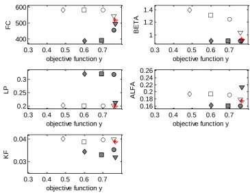
FIGURE 38: VALUES FOR ALFA IN REALISTIC SCENARIO WITH 95% CONFIDENCE INTERVAL ERROR BARS, OURTHE BASIN

FIGURE 39: VALUES FOR KF IN REALISTIC SCENARIO WITH 95% CONFIDENCE INTERVAL ERROR BARS, OURTHE BASIN

FIGURE 40: VALUES FOR ALFA IN REALISTIC SCENARIO WITH 95% CONFIDENCE INTERVAL ERROR BARS, CHIERS BASIN

(14)

FIGURE 43: FLOWCHART OF THE SEQUENTIAL STEPS OF THE SEM ALGORITHM (VRUGT ET AL., 2003B) FIGURE 44: SENSITIVITY ANALYSIS OURTHE

FIGURE 45: SENSITIVITY ANALYSIS CHIERS

FIGURE 46: VALUES FOR FC IN REALISTIC SCENARIO WITH 95% CONFIDENCE INTERVAL ERROR BARS, OURTHE BASIN

FIGURE 47: VALUES FOR BETA IN REALISTIC SCENARIO WITH 95% CONFIDENCE INTERVAL ERROR BARS, OURTHE BASIN

FIGURE 48: VALUES FOR LP IN REALISTIC SCENARIO WITH 95% CONFIDENCE INTERVAL ERROR BARS, OURTHE BASIN

FIGURE 49: VALUES FOR FC IN REALISTIC SCENARIO WITH 95% CONFIDENCE INTERVAL ERROR BARS, CHIERS BASIN

FIGURE 50: VALUES FOR BETA IN REALISTIC SCENARIO WITH 95% CONFIDENCE INTERVAL ERROR BARS, CHIERS BASIN

(15)

List of Tables

TABLE 1: PROPERTIES OF CLIMATE DATA IN OURTHE AND CHIERS RIVERS TABLE 2: PARAMETER VALUES

TABLE 3: PARAMETER VALUES AND RANGES AFTER CALIBRATION

TABLE 4: VALUES OF THE OBJECTIVE FUNCTIONS AFTER VALIDATION (VALUES CALIBRATION BETWEEN BRACKETS)

TABLE 5: OVERVIEW POSSIBLE RANDOM ERRORS IN DISCHARGE MEASUREMENT MEUSE RIVER (JANSEN, 2007) TABLE 6: LIST OF POSSIBLE ERRORS IN DISCHARGE DETERMINATION

TABLE 7: DIFFERENT VALUES OF PARAMETERS IN HYSTERESIS EFFECT TABLE 8: BOTTOM SLOPES OF THE OURTHE AND CHIERS RIVER TABLE 9: KEY CHARACTERISTICS OF FLOOD WAVES

TABLE 10: SPREAD DUE TO DIFFERENT VALUES FOR Α IN OURTHE AND CHIERS BASINS AND THE CORRESPONDING VALUES FOR Y

(16)

(17)

1

Introduction

In this chapter, an introduction of the research is presented. First, the background of the problem is explained in paragraph 1.1. Some similar previous studies are treated in paragraph 1.2. Together these elements lead to the problem description in paragraph 1.3. Subsequently the objective, research questions and used methodology are presented in that paragraph.

1.1

Background

Water institutes from all over the world have an important task of predicting future short-term and long-term discharges and water levels in river basins. An issue like climate change indicates the importance for adequate discharge and water level predictions. With adequate predictions possible threats can be estimated and the future risk of floods or droughts can be evaluated. For predicting the future discharges and water levels, hydrological models can be used. Hydrological models can be (semi-)distributed or lumped and can either be conceptual or physical.

A semi-distributed model is used if a basin can be separated into a number of sub basins and that each of these basins is distributed according to elevation and vegetation. A lumped model does not take into account the spatial variability of processes, input, boundary conditions and watershed geometric characteristics (Singh, 1995). If a model is conceptual, it means that the model parameters do not directly represent physical properties. That is why model parameters cannot be measured in the field. The model parameters which represent some basin characteristics are determined by calibration of the model. The advantage of a conceptual model is that it has a simple model structure. A disadvantage is that most parameters are empirical, which may reduce the validity of the model.

Before the model is applicable to predicting of future discharges in a certain river basin, the model has to be calibrated and validated. In the calibration process a set of parameters is estimated which results in the best simulation of the observed discharge, given sets of measured input data series. For this, discharge measurements are needed. These measurements are used as a reference.

Errors in input and output series may result in errors in estimated parameters and hence errors in simulated discharge. In particular, the effect of sampling errors in precipitation on the estimated parameters and simulated discharge has frequently been studied. The effect of discharge determination errors is less often investigated. More information about the influence of discharge determination errors on model performance and parameter estimation of a hydrological model can direct future discharge determination methods and research and may improve short- and long-term discharge predictions.

(18)

1.2

Previous research

As indicated in paragraph 1.1, in the past there has not been much research about the influence of errors in discharge determination on model performance and parameter estimation of hydrological models. In hydrological modeling, often an assumption is made there are no uncertainties in discharge data series or that the presence of uncertainties would not influence the behavior of the model. In this research, the fairness of this assumption is examined.

To investigate the uncertainties in discharge data and the influence of these uncertainties on the calibration of a hydrological model, it is important to learn from previous studies. One important aspect is that information has to be collected about uncertainties in discharge measurement. This part is mainly treated in chapter 3. Furthermore it can be useful to look at studies which focus on the uncertainties in input variables (incorrect or missing data) and their influence on model performance and parameter estimation. Other uncertainties in input and output of a hydrological model can be caused by applying a wrong spatial and/or temporal resolution. Studies that treat these kinds of uncertainties can contain useful elements for this research.

In studies regarding incorrect input data the focus is often on the quality of the precipitation data. An example of this is the research of Andréassian et al. (2001). They presented a method in which the quality of the precipitation data is assessed using quality functions. The GORE and BALANCE indices assess the quality of precipitation time distribution and the total depth respectively. The used hydrological models were GR3J, TOPMODEL and IHACRES, applied to three river basins, differing in surface area. The overall conclusion of this research was that with improving the quality of input data, the model performance increases.

Several previous studies are aimed at assessing the influence of varying spatial resolution of the rainfall input on model performance. Five of these researches are those from Bárdossy and Das (2008), Dong et al. (2005), Brath et al. (2004), Booij (2002b) and Bormann (2006). The first three were aimed at the distribution of rain gauges in a certain river basin. Bárdossy and Das (2008) investigated the influence of varying the distribution of the rain gauge network on model calibration using the HBV model. The outcome of these researches showed that if the rain gauge network changes, a new calibration of the HBV model parameters has to be performed. Specifically, the calibrated model with dense precipitation input fails when run with sparse precipitation information. On the other hand it turned out that a calibrated model with sparse rainfall information can perform well when run with dense precipitation information. Dong et al. (2005) and Brath et al. (2004) tried to find the optimal number of rain gauges in a catchment. Although different sizes of catchments were used (17 000 km2 and 1050 km2) the outcome of both researches was that the optimal number of gauges was five.

(19)

Bormann (2006) investigated the effect of spatial input data resolution on the simulated water balances and flow components using a multi-scale hydrological model, named TOPLATS. The conclusion of this research was that using a larger spatial resolution, the model performance decreases.

The studies mentioned above have their focus on uncertainties in input or spatial resolution in hydrological modeling and their influence on model performance. The problem is that no research is aimed at the influence of uncertainties in discharge data on model calibration. Some important elements from the previous studies that can be useful for this research are:

 In order to draw decent conclusions it is useful to focus on multiple watersheds, with differing properties;

 It is useful to use a ‘simple’ conceptual and/or lumped model, because in that case the influence of uncertainties can be evaluated relatively easy and the calculation time is limited. Furthermore, this research is one of the first studies that focus on uncertainties in hydrological modeling due to discharge measurement uncertainty. That is why it is logical to use a model that has a relatively simple structure;

 In the previous studies several objective functions are used, which assess the quality of a calibration. There are different kinds of objective functions, each with a certain focus on the hydrograph. For this research one or two objective functions have to be used, or they can be combined into one objective function;

 It is important to express the relationship between the magnitude of the uncertainties and the influence on model performance and/or the estimation of parameters.

1.3

Problem statement, objective, research questions and research model

The findings in previous studies lead to a problem that is stated below. This problem can be translated into a general research objective and three research questions.

1.3.1 Problem statement

The problem that is derived from the previous studies is that often an assumption is made that discharge uncertainties do not have any significant influence on model performance and model parameters after calibration. In this research it is examined whether this assumption can be justified.

1.3.2 Objective

The objective of this study is to investigate the influence of uncertainties in discharge determination on the estimation of the parameters and the performance of a lumped version the HBV model for two sub basins in the Meuse River, by applying an automatic global searching calibration method and using adapted observed discharge time series.

1.3.3 Research questions

The objective stated before leads to the following three research questions:

(20)

2. What kind of uncertainties in discharge determination can be present and how can these errors be brought into existing discharge time series?

3. What is the effect of uncertainties in discharge determination on model performance and parameter estimation of the HBV model applied to different sub basins of the Meuse River?

a. What is the effect of uncertainties in discharge determination on model performance of the HBV model, applied to different sub basins of the Meuse River?

b. What is the effect of uncertainties in discharge determination on the estimation of parameter sets of the HBV model, applied to these sub basins?

1.3.4 Research method

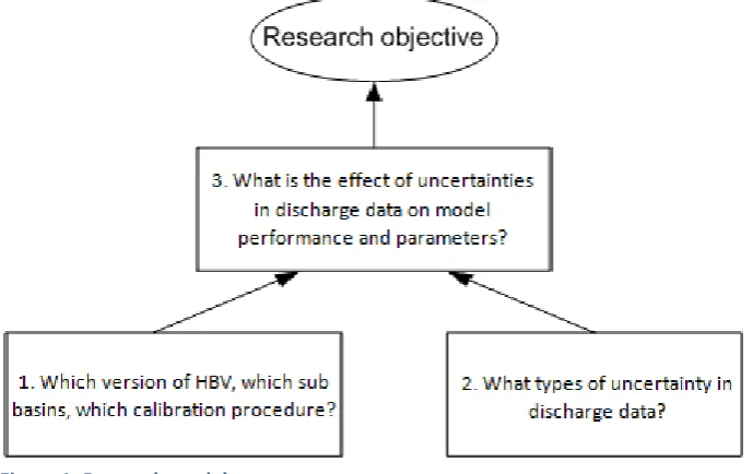
[image:20.595.71.416.317.534.2]

In Figure 1 a simple research model is given. The first two research questions form a foundation in order to be able to answer the third question. The third research question will directly contribute to the objective of the study.

Figure 1: Research model

Step 1 in this research is that data need to be collected and the hydrological model, sub basins and calibration procedure need to be chosen. Also a calibration is performed with the original discharge data. This ‘base case’ serves as a reference for future calibrations.

Step 2 in this research is to make an investigation about all possible uncertainties in discharge data. Subsequently for every error source a method is chosen about how the uncertainty can be integrated into an existing data set. This is done to simulate different kinds of discharge determination uncertainties. In this research an assumption is made that the original discharge data do not contain uncertainties or errors.

(21)

case’ calibration is used as a reference to assess the influence of the adapted discharge data on model performance and parameter sets of the HBV model.

1.4

Outline of the report

In Chapter 2 an answer is provided for research question 1. In this chapter the data collection and the reference HBV model is presented. At first the type and sources of data are explained. Also a choice for two sub basins of the Meuse is made and explained for these sub basins. After that, a description of the used rainfall runoff model, the HBV model, is given. Subsequently the calibration method that is used in the research is introduced. At the end of Chapter 2, the calibration and validation of the HBV model in the two sub basins is performed. This calibration and validation form the ‘base case‘, i.e. a reference for all following calibrations.

In Chapter 3 research question 2 is treated. This chapter contains some theory behind uncertainties in discharge determination. First, the origins of errors in discharge time series are explained. After that, a distinction is made between different types of errors. These different types of errors can be combined to several error sources. These four error sources are explained further and also a method is presented to introduce these errors into the original discharge data. These artificially constructed discharge time series are used subsequently to perform calibrations. The quality of the adapted discharge data series is quantified by two quality functions, which are defined at the end of Chapter 3. A part from the four error sources, a realistic scenario is developed.

In Chapter 4 the third and main research question is answered. In this chapter the results are presented and discussed. For each error source the influence of the errors on model performance and model parameters is shown. Also the results from the realistic scenario are analyzed and discussed.

(22)

(23)

2

Data collection and reference HBV model

In this chapter, the collection of the used data and the set up of the reference HBV model are discussed. In paragraph 2.1 the schematization of the chosen sub basins and the used data can be found. Paragraph 2.2 gives a description of the used hydrological model, the HBV-15 model. In paragraph 2.3 the used calibration procedure is explained. Paragraph 2.4 contains the calibration and validation of the base case, i.e. the situation with the original data, which results in a reference HBV model.

2.1

Data collection and schematizations sub basins

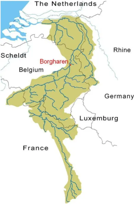
[image:23.595.183.410.263.611.2]

In Figure 2 the Meuse River Basin is shown (Riou vzw, 2010). The Meuse Basin is located in France, Luxemburg, Belgium, Germany and the Netherlands.

Figure 2: Meuse River Basin

In Figure 3 a schematization for the Meuse River Basin, upstream of Borgharen is given (Booij, 2005). The Meuse River Basin upstream of Borgharen can be de divided into several sub basins. The following 15 sub basins can be distinguished.

(24)

1: Meuse Lorraine sud 2: Chiers

3: Meuse Lorraine nord 4: Bar-Vence-Sormonne 5: Semoins

6: Viroin 7: Meuse midi 8: Lesse 9: Sambre 10: Ourthe 11: Ambleve 12: Vesdre 13: Mehaigne 14: Meuse nord 15: Jeker

Figure 3: Entire Meuse River basin upstream of Borgharen, containing Ourthe and Chiers (Booij, 2005)

A longitudinal profile of the Meuse River and its main tributaries is shown in Figure 4. In this figure the length and slopes of the tributaries can be found.

Figure 4: Longitudinal profile of the Meuse River and its main tributaries (Berger, 1992)

(25)

A difference between the basins is the average slope of the rivers, as shown in Figure 4. The slope of the Ourthe River is significantly steeper than the slope of the Ourthe River. Another difference, which is probably related to the slope of the rivers, is the shape of the discharge time series. While the Ourthe has a relatively low base flow and high peaks, the Chiers River has less high peaks and a higher base flow. This can be seen in Figure 5. In this figure daily measurement values of the discharge are shown for 10 years (1989-1998) for the Chiers and Ourthe rivers. The steeper slope of the Ourthe basin may be the reason for the extremer discharge regime of the Ourthe.

Figure 5: Discharge graphs Chiers and Ourthe Rivers

The average discharge in the basins is 23,0 and 25,5 m3/s respectively for the Ourthe and Chiers river, while the standard deviations of the discharges are respectively 29,8 and 23,4 m3/s. These values indicate that the average discharge is higher in the Chiers River, but that the Ourthe River shows a more extreme behavior.

The climate data, such as daily average precipitation, temperature and potential evapotranspiration, are of comparable magnitude between the basins. This is shown in Table 1. The mean and standard deviation from the available daily data are calculated and it turns out that there is not much difference in input variables between the basins.

Table 1: Properties of climate data in Ourthe and Chiers rivers

Climate data Ourthe Chiers

Precipitation [mm] Mean 2.7 2.6 Standard deviation 4.7 4.7

Temperature *⁰C+ Mean 8.6 9.2 Standard deviation 6.5 6.6

PET [mm] Mean 1.5 1.6

Standard deviation 1.5 1.3

2.2

HBV model

The used hydrological model in this research is the HBV model. This model is developed in 1972 by Bergström. Initially, the model was developed for the forecasting in hydropower developed rivers of

0 500 1000 1500 2000 2500 3000 3500 0 50 100 150 200 250 300 350 400 Chiers time (days) d is c h a rg e ( m 3 /s )

(26)

Scandinavia (Bergström, 1976). Since then, the model has been applied in more than 50 countries and regions in the world (Bergström, 1995).

In this research, a lumped version of the HBV model is used, the so called HBV-15 model, developed by Booij (2002a). In the research of Booij (2002a) 15 sub basins of the Meuse River upstream of Borgharen were used. In the HBV-15 model, each of the 15 sub basins is schematized without spatial variability. So, for every sub basin a lumped model is used and these 15 lumped models are linked and together form the HBV-15 model. In this research just two of these sub basins are considered, so two of these lumped models are used. In the following sections a description of this version of the lumped HBV model is given. For this research, the HBV model is programmed into MATLAB.

2.2.1 Description HBV model

In general, the HBV model is a conceptual, rainfall-runoff model and can be used as a semi-distributed or lumped model. It was developed at the Swedish Meteorological and Hydrological Institute (SMHI) in the early 70s (Bergström, 1976; SMHI, 2003). A lumped version of the HBV model is chosen for this research because of its conceptual, simple model structure. Because there has not been much research in the past that considers uncertainties due to discharge measurement errors, a choice is made for a simple model which is easy to use. A semi-distributed model is used if a basin can be separated into a number of sub basins and that each one of these is distributed according to elevation and vegetation (Singh, 1995). In this research the choice for a lumped version of the HBV model for the Ourthe and the Chiers rivers is made and it does not take into account the spatial variability of processes, input, boundary conditions and watershed geometric characteristics.

The used HBV is called conceptual because the model parameters do not directly represent physical properties. That is why model parameters cannot be measured in the field. The model parameters, which indirectly represent the basin characteristics, are determined by calibration of the model. The advantage of a conceptual model is that it has a relatively simple model structure. A disadvantage is that most parameters are empirical, which may reduce the validity of the model.

(27)

Soil Box

Upper Response Box

Lower Response Box

P R E C IP IT A T IO N E V A P O T R A N S P IR A T IO N R e c h a rg e C a p illa ry F lu x Slow response Quick response Total discharge P e rc o la tio n FC Soil moisture BETA LP CFLUX KF ALFA KS PERC Ground water

Deep ground water

R a in S n o w TEM_PER ATU_RE

Figure 6: Schematization of the used HBV model

2.2.2 Description of the lumped HBV model

Figure 6 shows the schematization of the model. The lumped version of the HBV model consists of three routines: the precipitation routine, the soil moisture routine and the runoff generating routine, which can be divided into quick and slow runoff. These routines are discussed below (Bergström, 1976).

Precipitation Routine

The precipitation, which is the initial input of the model, is divided into rainfall and snowfall. If the temperature is above a certain threshold, rainfall will be present. Below this threshold, the precipitation consists of snowfall. Also the melting and refreezing processes are taken into account in this routine.

Soil Moisture Routine

This routine controls which part of precipitation is evaporated or stored in the soil. The ratio of actual soil moisture (SM) and the maximum water storage capacity of the soil (parameter FC [mm]), and the soil routine parameter (BETA [-]) together assess the runoff coefficient. With this runoff coefficient, the part of the precipitation P which forms the recharge R to the upper response box can be calculated, by using equation (1). If the soil is saturated (SM=FC), then the recharge is equal (if

BETA=1) or larger (if BETA>1) than the precipitation, dependent on the value of BETA.

) ( * )

( P t

(28)

LP [-] describes the limit of water storage for potential evapotranspiration. Above this limit, potential and actual evapotranspiration will be equal to the potential evapotranspiration. Data for potential evapotranspiration are input for the HBV model. The parameter CFLUX [mm day-1] represents the maximum capillary flux from the runoff routine into the soil.

Runoff Generation Routine (quick and slow runoff)

The runoff generation routine is the response function that transforms excess water from the soil routine to runoff. The runoff generation routine consists of two reservoirs. The first one, the upper response box, is a non-linear reservoir which represents the quick runoff. KF [day-1] is a recession parameter in the upper or fast response box. ALFA [-] is a measure for non-linearity of the quick runoff.

The second reservoir is the linear lower response box. This box represents the slow response (with recession coefficient KS [day-1]), i.e. the base flow that is fed by groundwater. The fast (Qf[mm/day], equation (2)) and slow (Qs [mm/day], equation (3)) response can be characterized by the following equations, in which Sf [mm] and Ss [mm] represent the storage in respectively the fast and slow response box.

) 1 (

)

(

*

)

(

_f ALFA

f

t

KF

S

t

Q



 (2)

)

(

*

)

(

t

KS

S

t

Q

s



s (3)

Groundwater recharge is ruled by a maximum amount of water that is able to penetrate from soil to groundwater (parameter PERC [mm day-1]) through the upper response box.

2.3

Calibration procedure

For the calibration procedure an optimization method and an objective function have to be chosen for the research. Choices for these elements of the calibration are explained in the following sections.

2.3.1 Optimization method: SCEM-UA

The used method for model optimization is the SCEM-UA algorithm. This method has been developed by Vrugt et al. (2003a). SCEM-UA is an automatic global searching method which is based on the SCE-UA algorithm (Singh, 1995). Instead of using the Downhill Simplex method that is used in the SCE-UA algorithm, an evolutionary Markov Chain Monte Carlo (MCMC) sampler is used. This means that a controlled random search is used to find the optimum set of parameter values in the parameter space. The choice for the SCEM-UA method is based on the fact that it is an automatic global searching method that converges quite fast to the optimal value. An advantage of this algorithm is that the chance of finding the global optimum is very high. In Appendix 1 more information about the SCEM-UA method can be found. The SCEM-UA method is also programmed into MATLAB and linked with the HBV model. This makes that all optimizations in this research take place in the MATLAB program.

(29)

research. The parameters which do not have much influence on model performance get a fixed value. This results in a smaller calibration time, as the SCEM-UA method needs less iterations to find the optimum. When an optimum is found after calibration, this model with parameter set and objective function is used as a reference or ‘base case’ in this research.

2.3.2 Objective function

There are different kinds of objective functions which can determine the model performance given a certain parameter set. In calibrations single or combined objective functions can be used. A single objective function is an objective function which is aimed at a specific property of the hydrograph. Some objective functions for example assess the quality of the shape of the hydrograph or a correct water balance over the entire calibration period. Other functions evaluate the quality of specific parts of the hydrograph, such as peak flows or low flows. In this research it is important to have a good representation of the entire hydrograph. It is also useful to have a correct water balance. This is why a combined objective function will be used. This combined objective function combines the single objective functions NS and RVE (Nash and Sutcliffe, 1970). The functions NS and RVE are shown in equation (4).











 





_N i obs i obs N i i obs i sim

Q

t

Q

t

Q

t

Q

NS

1 2 1 2

)

(

)

(

)

(

1

and











 





_N i i obs N i i obs i sim

t

Q

t

Q

t

Q

RVE

1 1

)

(

)

(

)

(

(4)

Where

Q

_obs

(

t

_i

)

and

Q

_sim

(

t

_i

)

are observed and simulated daily discharge at time step

t

irespectively

and

Q

obs is mean observed daily discharge and

N

is the total number of time steps. NS assesses the

quality of the shape of the hydrograph and has a value of 1 if a perfect match in hydrograph is present, while RVE is aimed at the relative volume difference between the observed and simulated discharge and has an optimal value of 0.

The combined objective function used in this research is called y (Akhtar et al., 2009) and defined as follows:

RVE

NS

y





1

(5)

In case of an optimum, NS has a value of 1 and RVE has a value of 0. This makes that the optimal situation has a value of 1 of the objective function y.

2.3.3 Calibration time period

(30)

2.4

Calibration and validation results, reference HBV model

In this paragraph the reference HBV model is set up. The calibrations of the model with the original data of the two sub basins form the ‘base cases’ or reference models for this research. Therefore at first the calibration with all eight parameters takes place and after performing a sensitivity analysis this calibration is further optimized and subsequently validated for both basins.

2.4.1 Calibration with 8 parameters

In the first calibration, eight model parameters are used to optimize the model. Some parameters are more sensitive than other parameters. In other words, some parameters have a larger influence on the objective function than other parameters. That is why these parameters need more attention in a calibration. To select the most influential parameters, a univariate sensitivity analysis is performed. This means that the variables are varied once at a time while the other parameters keep a constant value. In Table 2 an overview of the parameter values and ranges is given. The ranges of the Ourthe basin are based on the research of Booij and Krol (2010). Initially, the ranges for the Chiers basin were also coming from this research, but it seemed that this did not deliver the maximum value for the objective function, because for some parameters the optimal parameter value was situated at the border of the parameter range. This might be an indication that the real optimal parameter value is lying outside the parameter range. To solve this problem, the parameter range is changed in a way that the optimal value is not at the boundary of the range any more. The parameter ranges after the modifications still contain realistic values and therefore are suitable for calibration.

Table 2: Parameter values

Parameter [unit]

Physical interpretation Range

Ourthe Basin Range Chiers Basin Optimal value Ourthe Optimal value Chiers

FC [mm] Maximum soil moisture storage 150 – 500 400 – 700 224 485

BETA [-] Shape parameter of runoff generation 1 – 3 0.9 – 1.5 1.907 1.157

LP [-] Fraction of FC above which potential evapotranspiration occurs and below which evapotranspiration linearly reduces

0.2 – 1 0.1 – 1 0.388 0.259

ALFA [-] Measure of non-linearity for fast flow 0.1 – 1.5 0.05 – 0.5 0.505 0.202

KF [day-1] Recession coefficient for fast flow reservoir

0.005 – 1 0.005 – 1 0.0219 0.0328

KS [day-1] Recession coefficient for slow flow reservoir

0.005 – 1 0.005 – 1 0.0069 0.005

PERC [mm day-1]

Drainage from the fast flow reservoir to the slow flow reservoir when sufficient water is available

0.1 – 2.5 0.1 – 2.5 0.569 0.326

CFLUX [mm day-1]

Maximum value for capillary flow 0.1 – 2.5 0 – 2.5 1.363 0.454

Value objective function 0.933 0.759

2.4.2 Sensitivity analysis

(31)

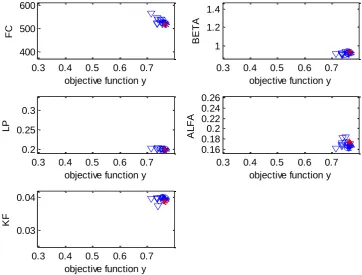
change. The parameters which are less sensitive on model performance will get a fixed value in further calibrations in this research, because this leads to a decrease in calibration time. In the sensitivity analysis each parameter is varied one at a time, while the other seven are kept constant. The variations of the parameters influence the model in a way which results in a change in objective function. In Appendix 2 the outcome of the sensitivity analyses of both sub basins is shown.

In both the Ourthe and Chiers basins the most sensitive parameters are ALFA, FC, LP, BETA and KF. These parameters are chosen to optimize the calibration. CFLUX, PERC and KS are not sensitive in the Ourthe and Chiers basins with the present climate and discharge data and will get the values as shown in Table 2 as a fixed value in the calibrations in this research.

In a study of Booij and Krol (2010) the three parameters ALFA, FC and LP are considered the most identifiable for the Ourthe and the Chiers basins. This means that these parameters are most sensitive to a certain combined objective function in which the single objective functions NS, RVE,

NSL and NSH (Nash Sutcliffe coefficients for relatively low and high flows) (Nash and Suttcliffe, 1970) were included.

(32)

2.4.3 Optimization by calibration of the five most sensitive parameters

As seen in section 2.4.2 the parameters FC, BETA, LP, ALFA en KF are used in the calibration of both the Chiers and Ourthe basins. In the sensitivity analysis, the used ranges were rather large. To perform a more accurate calibration, the ranges are made narrower. The minimum and maximum values of the parameters are based on the parameter values from the first calibration (shown in Table 2). The minimum value is 80% of the original value, and the maximum value is 120% of this value. In Table 3 the ranges of the five calibration parameters that are used for the final calibration are shown. The other three parameters get a fixed value which is also shown in the table. The maximum number of iterations in the SCEM-UA algorithm in this calibration is 1500.

Table 3: Parameter values and ranges after calibration

Parameter [unit]

Range/value Ourthe Basin

Range/value Chiers Basin

Optimal value Ourthe

Optimal value Chiers

FC [mm] 179 – 268 388 – 583 211 520

BETA [-] 1.52 – 2.29 0.90 – 1.40 1.71 0.94

LP [-] 0.31 – 0.47 0.20 – 0.32 0.310 0.202

ALFA [-] 0.40 – 0.61 0.16 – 0.25 0.559 0.175

KF [day-1_] _{0.017 – 0.027} _{0.026 – 0.040} _0.0175 _0.0388

KS [day-1] 0.0069 0.005 0.0069 0.005

PERC [mm day-1]

0.569 0.326 0.569 0.326

CFLUX [mm day-1]

1.363 0.454 1.363 0.454

Values objective functions y 0.934 0.767

NS 0.934 0.767

RVE 0.002 % 0.000 %

Table 3 shows the values of the parameters after optimization, as well as the values for the combined objective function y and the functions NS and RVE. The Ourthe basin has a significantly higher value for the objective function compared to the Chiers basin. This means that the HBV model has more difficulties in simulating the discharge of the Chiers basin compared to the Ourthe, given the climate data. The reason for that can be that the quality of the data in the Ourthe basin is better, or that the HBV model is more suitable for rivers with a relatively low base flow and high peaks like the Ourthe, i.e. more extremes and variability.

The value for RVE is very small in both basins. The use of this particular combined objective function

y implies that it is important that the water balance over the entire calibration period corresponds with the real situation.

(33)

In Figure 7 and Figure 8 show the outcome of the calibrations of the two basins. The blue dots represent daily discharge measurements and the red graph represents the simulated data.

19840 1986 1988 1990 1992 1994 1996 1998 2000

50 100 150 200 250 300 350 400 time (year) D is c h a rg e ( m 3 /s ) Simulated Measured

Figure 7: Calibration Ourthe basin period 1984 – 1998

19840 1986 1988 1990 1992 1994 1996 1998 2000

20 40 60 80 100 120 140 160 180 200 time (year) D is c h a rg e ( m 3 /s ) Simulated Measured

Figure 8: Calibration Chiers basin period 1984 – 1998

(34)

flows. The peaks tend to be underestimated by the model, while the low flows are often overestimated.

All parameters in the HBV model have a physical background. Below, for each parameter the comparison of the differences in parameter value between the basins is made. In paragraph 2.1 the differences between the hydrographs of the two basins are explained. Figure 5 showed that the Ourthe has a relatively low base flow and high peaks, the Chiers river has less high peaks and a higher base flow.

FC

The Chiers basin has a higher value for FC than the Ourthe basin. This means that maximum soil moisture storage is higher in the Chiers basin. This higher value means that there is a possibility of buffering if there is a lot of precipitation. This will lead to less high and steep peaks in the Chiers river compared to the Ourthe. The discharge data of the two rivers confirms this expectation.

BETA

BETA is a parameter which describes the relative contribution of precipitation from the soil moisture box to the upper response box (recharge) if the soil moisture box is not saturated. If BETA has a high value, the recharge is smaller in case of a moisture deficit in the soil box than with a low value of

BETA. The value for BETA is highest in the Ourthe basin, which means that given a certain soil moisture deficit and precipitation, less recharge will occur in this basin compared to the Chiers basin. As a result, the upper response box in the Chiers will be filled faster than in the Ourthe basin. It is difficult to clarify what is the influence of this on the discharge regime.

LP

LP represents the fraction of the maximum soil capacity (FC) above which potential

evapotranspiration occurs and below which evapotranspiration linearly reduces. So if LP is high, the chance that the actual evapotranspiration is equal to the potential evapotranspiration is smaller than in cases LP has a low value. So in the basins with a high LP, most of the time the actual

evapotranspiration is less than the potential evapotranspiration. Because LP is a fraction of FC, the effect of a certain value of LP also depends on the value of FC. The Ourthe has a bigger value for LP

than the Chiers basin, but also has a smaller value for FC, which indicates that the Ourthe basin has a smaller field capacity. LP has a slightly higher value in the Ourthe basin compared to the Chiers, but since the value of FC is smaller in the Ourthe it is difficult to determine in which basin the most evapotranspiration takes place and what is the influence of this on the hydrograph.

ALFA

The value of ALFA is higher in the Ourthe basin. This means that at a certain change in storage in the upper response box the quick response has a more non-linear behavior in the Ourthe basin compared to the Chiers basin. This means that if the storage increases, so if precipitation is present, the quick discharge faster increases. In these basins the Ourthe has the highest and steepest peaks and the parameter ALFA confirms that.

KF

(35)

Considering the hydrographs of the rivers, it makes sense that KF has a higher value in the Chiers basin, because it has larger discharges at low flows compared to the Ourthe basin.

KS

For the parameter KS a same conclusion can be drawn. In contrast with KF, this parameter has a linear relation with the slow flows from the lower response box. The values do not vary much between the two basins. The Ourthe basin has a higher value. The effect of this value on the discharge regime is difficult to determine.

PERC

The value of PERC is higher in the Ourthe basin. This means in the Ourthe basin there is more percolation from the upper response box into the lower response box. It is difficult to estimate the influence of the difference between the basins on the hydrograph.

CFLUX

The value of CFLUX is considerably higher in the Ourthe basin, so in this basin there is more capillary flux from the upper response box into the soil moisture box. So if the soil moisture is smaller than the field capacity, the vertical flux from the upper response box into the soil is bigger in the Ourthe basin.

The influences of the values of the last three parameters on the hydrograph are difficult to clarify. However these parameters are less important in this research, as they are not of importance in the rest of this research, because their insensitivity in these basins.

(36)

0 500 1000 1500 100 200 300 F C [ m m ]

0 500 1000 1500

1.5 2 2.5 B E T A [ -]

0 500 1000 1500

0.35 0.4 0.45 L P [ -]

0 500 1000 1500

0.4 0.6 0.8

number of iterations

A L F A [ -]

0 500 1000 1500

0.01 0.02 0.03

K F [ 1 /d a y ]

Figure 9: Development of the parameters in the calibration of the Ourthe basin

0 500 1000 1500

200 400 600 F C [ m m ]

0 500 1000 1500

0.5 1 1.5 B E T A [ -]

0 500 1000 1500

0.2 0.3 0.4 L P [ -]

0 500 1000 1500

0.2 0.25

A L F A [ -]

0 500 1000 1500

0.02 0.03 0.04

K F [ 1 /d a y ]

(37)

The figures show that in the Ourthe basin the parameters FC, ALFA and KF have a strong convergence in the beginning of the calibration, while the optimizing algorithm seems to have more difficulties in determining BETA and LP. FC, ALFA and KF are therefore well identifiable.

In the Chiers basin FC, BETA and LP show a strong convergence and thus are well identifiable, while

(38)

2.4.4 Validation

In the validation, the parameter values of the calibration are used. The validation period is from 1968 to 1983. In this time span there are a couple of periods in the Chiers basin in which no measurement data are present.

In Figure 11 and Figure 12 the outcome of the validation of respectively the Ourthe and the Chiers basin is shown. The blue dots are the daily determined discharge values and the red graph is the simulated discharge. If discharge data are unavailable, no blue dots are present. The figures also show the values of the objective functions NS, RVE and y. The objective functions are only calculated over the periods in which measurement data are present.

19680 1970 1972 1974 1976 1978 1980 1982 1984 1986

50 100 150 200 250 300 350

time (year)

D

is

c

h

a

rg

e

(

m

3

/s

)

Simulated Measured

(39)

19680 1970 1972 1974 1976 1978 1980 1982 1984 1986 20

40 60 80 100 120 140 160 180 200

time (year)

D

is

c

h

a

rg

e

(

m

3

/s

)

Simulated Measured

Figure 12: Validation Chiers basin period 1968 – 1983

In Table 4 the values of the combined objective function, as well as the functions NS and RVE are shown. The values of the objective functions in the calibration of the base case are shown between brackets.

Table 4: Values of the objective functions after validation (values calibration between brackets)

Ourthe Chiers

y 0.842 (0.934) 0.752 (0.767)

NS 0.849 (0.934) 0.785 (0.767)

RVE 0.90 % (0.002%) 4.44 % (0.000%)

The validation over the period 1968 to 1983 yields an objective function y of 0.842 for the Ourthe basin, while the objective function in the calibration had a value of 0.934. However, 0.842 is still a good value for the validation. In the Chiers basin, the objective function y has a value of 0.752. This value is comparable with the objective function in the calibration, which was 0.767.

(40)

(41)

3

Methodology: uncertainties in discharge determination

Uncertainties in discharge time series are present due to errors in discharge determination. In paragraph 3.1 a number of possible types of errors are discussed. In paragraph 3.2 these errors are classified into different sources of errors. These error sources contain one or a couple of the possible errors. This classification is set up to construct discharge time series including errors. These artificial discharge series are used in the research to analyze the influence of the error sources on model performance and model parameter estimation. A part from the classification of the errors, paragraph 3.2 also contains descriptions of integrating the types of errors into the discharge series. An assumption is made that the original discharge data do not contain errors. The different error sources lead to a “realistic scenario”, which is expected to approach the real situation best. This realistic scenario is treated in paragraph 3.3. In paragraph 3.4 a method for quality assessment of these discharge series is presented. These classification functions give an estimation of the quality of the artificial time series compared to the original time series.

3.1

Errors in discharge time series

There are different kinds of errors which can cause deviations form the real discharge time series. In general, there are two types of errors. The first type of error occurs at the execution of the measurement. This is explained in section 3.1.1. Furthermore, the use of the Q-h relation can bring errors into discharge data, which is clarified in section 3.1.2.

3.1.1 Measurement errors

Errors which originate during the execution of the measurement are referred to as measurement errors. Measurement errors can have different causes. The estimate of the discharge at a certain moment is determined by measurements of the water level, cross section and/or velocity. Uncertainties that can occur during the measurements of these elements are (Jansen, 2007):

 Uncertainty in measured data (empirical quality);

The difference between measured discharge and actual discharge is caused by random and systematic errors. The random error can be indicated as the spread in the measurement. The random errors can occur with or without a certain autocorrelation.

 Uncertainties regarding the executing of the measurement (methodological quality) ;

There are different reasons for a bad execution of the measurements. In extreme conditions like high water levels, standard procedures cannot be followed and errors can occur. Other reasons for a bad execution can originate if a certain flow is completely different from uniform flow, while an assumption is made that the flow is uniform.

 Uncertainties regarding the performance of the measuring equipment;

As a consequence of breaking down or failing of measurement equipment, an instrument can malfunction.

(42)

Measurement errors can be systematic or random, but in reality a combination of random and systematic errors might be present. A random error can be completely random or can contain autocorrelation. This means that the error at a certain time step has influence on the error of the next time step. In the following sections, the systematic and random errors (with and without autocorrelation) are further explained.

Systematic error

Systematic errors are errors which are caused by incorrect use of the measuring instruments or by a defect in the instruments. A systematic error can either have a fixed absolute or relative deviation from the real value.

Random errors, with or without autocorrelation

A random error is caused by unknown unpredictable changes in the measurement. This can occur in the measurement equipment or can originate from external conditions. An assumption is made that these random errors are normally distributed with a certain mean and standard deviation (Jansen, 2007). In discharge measurement, random errors can have an autocorrelation in time. This means that the error depends on the error of the previous day. Random errors without autocorrelation have a mean of 0.

Table 5 shows the possible random errors in discharge measurement. The values of the spread of the random errors are found in the research of Jansen (2007). This research is based on measurement methods in de Meuse River at St Pieter, Borgharen and Maastricht. It is not clear what kind of measurement techniques are used in the Ourthe and Chiers rivers. That is why in this research several values for the spread in discharge for random errors will be used. The spread is defined as the maximum deviation in discharge of the measurements from the real values in 95% of the points, assuming a normal distribution of the errors.

Table 5: Overview possible random errors in discharge measurement Meuse River (Jansen, 2007)

Measurement error Present in

period

Location of error Spread in discharge of

random error

(percentage of points in 95% confidence interval)

Level scale 1917-1956 Water level 10%

Level scale 1956-1975 Water level 5%

Registering level writer 1975-2000 Water level 5%

Digital level gauge 2000-2006 Water level 5%

ADM 2000-2006 Discharge 2.5%

Level stick and angustifolia posts

1917-1956 Cross section 2%

Measurement vessel and GPS

2000-2006 Cross section 1%

3.1.2 Errors from using Q-h relation

(43)

Q-h relation can Q-have influence on tQ-he discQ-harge estimation. In tQ-he following sections tQ-hese errors are discussed briefly.

Properties of a high water event

High water waves which last for a long period will have a different discharge compared to shorter waves with an equal water level. The differences are mainly noticeable at the peak of the wave. Steep and short high water waves will result in an underestimation of the discharge when applying the Q-h relation, while long and gradually increasing waves result in an overestimation of the discharge. This is due to the steepness of the wave. The steepness of the front of the wave has a relation with the celerity of the wave and therefore with the flow velocity. The changes in velocity that are a result of this, cause significant differences in water level in case of high water.

Hysteresis

The hysteresis effect describes the phenomenon in which the discharge in a hydrograph at a certain water level is higher if the water level is increasing, than in case the water level is decreasing, compared to the equilibrium situation (Boiten, 1986). This can be explained as follows: If a high water wave passes, diffusion occurs because a certain gradient in water level arises. This means that the peak of the wave, i.e. the flood maximum (the location with the highest discharge), gets a little smoother. The streaming velocity increases somewhat in front of the wave and thus the water depth decreases a little on that location. So at a certain fixed point along the river, the maximum discharge occurs at a certain moment, but the maximum water level occurs somewhat later (Jansen et al., 1979). The hysteresis effect is graphically shown in Figure 13. This figure shows that if a high water wave passes at a certain fixed point along the river, the maximum value for the discharge Q occurs earlier in time than the maximum value for the water level h. This means that at a certain water level

h different values for the discharge Q can occur, depending on the presence of a rise or a fall in water level.

(44)

Outdated Q-h relation

If the Q-h relation loses its validity because it is outdated, different systematic errors can be present in the relation. The measured water level will not represent a correct value of the discharge. After some time a systematic error can be arisen. This systematic error can represent changes in the cross section of the river. For example, if sedimentation takes place at a certain location, the water level will be higher at a certain discharge compared to the water level before the sedimentation.

The different types of errors are summed up in Table 6.

Table 6: List of possible errors in discharge determination

Location of error Error

Discharge measurement (a) Systematic errors

(b) Random errors without autocorrelation (c) Random errors with autocorrelation Q-h relation (d) Properties of a high water event

(e) Hysteresis effect (f) Outdated Q-h relation

An addition to this overview, a combination of the two locations of the errors can be distinguished. When using the Q-h relation measurement errors in the water level h can be made. According to RIZA the spread of the random error in discharge determination when using the Q-h relation is between 5% and 10% (Jansen, 2007). This kind of error is not treated separately, because it will have a similar outcome as the random errors.

3.2

Sources of errors

In reality, combinations of the errors shown in Table 6 occur in discharge determination. To perform a realistic analysis, different errors are grouped by its source. These sources are developed because it is not clear what method is used for discharge determination in the Ourthe and Chiers basins. Error sources 1 and 2 are aimed at errors in discharge measurement itself, while sources 3 and 4 are cases in which the Q-h relation is used.

Measurement uncertainties:

 Error source 1: combination of a systematic error (a) and entirely random errors (b) in discharge, water level or cross section;

 Error source 2: Random errors with autocorrelation in time. These errors can be present in discharge, water level and cross section (c);

Q-h relation errors:

 Error source 3: use of Q-h relation with the uncertainties of the properties of a high water event (d) and the hysteresis effect (e);

 Error source 4: use of an outdated Q-h relation (f);

(45)

adapted discharge time series are used in the calibration of the HBV model. The results of those calibrations can be found in chapter 4.

3.2.1 Error source 1: Combination of systematic and random errors

In this error source, a combination of systematic errors and random errors without autocorrelation is present. These errors can be a result of measurement errors in discharge, cross section or water level, but can also originate from the use of the Q-h relation, in which only the water level is measured.

Random