Munich Personal RePEc Archive
Do balanced-budget rules increase
growth?
Stone, Joe
University of Oregon
20 July 2014
Online at
https://mpra.ub.uni-muenchen.de/57605/
1
DO BALANCED-BUDGET RULES INCREASE GROWTH?
Joe A. Stone Economics University of Oregon
July 2014
ABSTRACT.
This study tests the hypothesis that balanced-budget rules (BBRs) that restrict public borrowing
to investments in public infrastructure increase growth by increasing the productivity of debt,
either because investments in public infrastructure are more productive than other uses for which
states borrow funds or because BBRs lower borrowing costs. Results are based on data at 5-year
intervals for 49 US states over the period 1957-2007. The tests strongly support the hypothesis
that BBRs increase growth by increasing the productivity of debt and withstand a variety of
robustness checks, including alternative lags, exogeneity tests, GMM estimation, a placebo test,
and the influence of outliers.
Keywords: balanced budget rule, infrastructure, fiscal policy, regional growth.
2
I. INTRODUCTION
Soaring levels of debt in Europe and in the United States have spurred interest in
balanced-budget rules (BBRs). The primary economic objection to BBRs is that they overly
restrict fiscal policy by preventing tax smoothing and impeding stable growth. Not surprisingly
then, BBRs are rare among central governments. However, they are common at the sub-national
level in the United States, where every state but Vermont has some type of BBR and restriction
on debt. Paradoxically, BBRs do not necessarily balance state budgets, for reasons noted by
Bohn and Inman (1995); Inman (1996); and Reuben and Poterba (1999).
Many BBRs for example, only apply ex ante, so officials tend to overestimate revenues
and underestimate expenditures, reducing the extent to which the rules limit fiscal flexibility
during a budget cycle; and even when BBRs apply ex post, officials often resort to temporary
accounting manipulations to avoid a deficit. Moreover, most states only apply BBRs to current
operations and exempt budgets for public infrastructure projects financed by long-term bonds. In
addition, BBRs vary in whether they require the governor to submit a balanced budget to the
legislature and whether require the legislature is required to pass a balanced budget. BBRs
typically incorporate similar limitations for other public entities subject to state jurisdiction.
Evidence that BBRs do not necessarily balance budgets begs the question: Why did states
put the rules in place? Wallis and Weingast (2006) (WW) argue that the primary purpose of
BBRs is to restrict borrowing to growth-enhancing investments in infrastructure, not simply to
balance budgets. WW offer historical and economic context to support their argument, but no
study has linked the stringency of BBRs directly to higher growth through an increase in the
3
complementary channels: by redirecting borrowing from less to more productive expenditures or
by lowering the cost of servicing debt.
Several attributes of BBRs, debt, and the hypothesized influence of BBRs on the growth
effect of debt aid identification. 1) Most states lodged BBRs and debt-limitation rules in their
constitutions long ago in the nineteenth or early twentieth century and now rarely make changes;
2) The stringency of state BBRs varies greatly. 3) The hypothesized effect is a nonlinear
interaction between debt and the presence and stringency of BBRs, which permits the effect of
the BBR-debt interaction to be separated from the direct effect of debt. Lastly, 4) the stock of
state and local debt tends to accumulate slowly over time, so that both debt and BBRs are
predetermined, if not strictly exogenous. We exploit these attributes using several alternative
estimation strategies.
II. OTHER EFFECTS OF BBRS
Several other empirical effects of BBRs are already well documented. Reuben and
Poterba (1999) find that balanced-budget and debt-restriction rules lead to lower taxes and lower
debt, and Alt and Lowry (1997) find that more stringent BBRs are associated with lower
borrowing costs. Despite concern that BBRs limit fiscal flexibility needed for counter-cyclical
policies, Levinson (1997), Alesina and Bayoumi (1996), and Krol and Svorny (2007) provide
mixed evidence to resolve the issue; Carlino and Inman (2013) find significant power for
countercyclical deficits but do not focus on the role of BBRs, Both they and Eberts and Stone
(1993) offer evidence that suggests an explanation for the conflicting results on whether or not
BBRs increase the volatility of state and local economies: countercyclical deficits are less
effective in the long run because they induce a subsequent reversal, offsetting earlier effects.
4
III.1 Endogenous-growth models
Endogenous-growth models along the lines of Barro (1989), Adam and Bevan (2005),
Checherita, et al. (2012), Grenier (2013), and Greiner and Fincke (2012)—to mention only a
few, have proven to be a useful framework for both theoretical and empirical studies of the
effects of state fiscal structures on growth. Unlike traditional neoclassical models, endogenous
growth models permit a permanent change in fiscal structure to have a permanent effect on
growth rates. While providing valuable insights, these studies yield widely varying results for the
link between growth and public debt—zero, positive, negative, and inverse U-shaped.
Fortunately, the validity of the hypothesis tested here rests on whether BBRs make the effect of
debt on growth significantly less negative or more positive, not on whether the direct effect of
debt is zero, positive, or negative.
To apply closed-economy endogenous growth models to the open-economy environment
of state and local economies we assume that states are quasi-open economies with goods and
factors that respond sluggishly over our recursive lag interval (ten years). In a typical
endogenous-growth model, output growth in the steady state depends only on structural
parameters and fiscal structures, such as taxes and other elements of the government budget
constraint. The stock of private capital is endogenously determined in these models, so it does
not appear as an independent variable.
III.2 Neoclassical-growth models
Mutatis mutandis, the structural parameters and exogenous variables are common to both the
neoclassical- and endogenous-growth models. We rely on the latter as the framework for our
5
models, but because the endogenous-growth models permit permanent changes in fiscal structure
to have persistent effects, providing a rationale for our recursive structure with long-lags.
IV. DATA AND EMPIRICAL SPECIFICATION
Our baseline empirical specification is adapted from Bleaney and others (2001), Bania and others
(2007), and Gray and Stone (2012). It is presented below as equation (1). We specify an
equation incorporating fixed effects for state-specific growth common to all periods,
period-specific factors common across states, as well as period-period-specific factors unique to each state. In
this context, current and lagged unemployment rates are expedient because they are cyclically
sensitive to state- and regional-specific factors but mean reverting. We employ an index
constructed by the Advisory Commission on Intergovernmental Relations (ACIR, 1987) as a
measure for the stringency of BBRs. We use this index rather than the measure constructed by
the U.S. General Accounting Office because the former is almost universally adopted and semi
continuous, rather than simply dichotomous (strict or not).1 We rely on a long j-interval,
recursive structure, where j alternately equals one (five years) or two (ten years), as well as an
error-correction term.
IV.1 Baseline specification
Our baseline empirical specification is equation (1):
(1) Vit =c +ci +ct +b1dit-j +b2Di t-j +b3ACIRi*Dit-j +B1Xi (t-j) +B2Zit + eit
1Krol and Svorny (2007) identify anomalies in the two measures, but they are not directly
comparable: the KS index is dichotomous (strict or lenient), the ACIR index is semi continuous.
6
Where (Vit) is the change in the log of real personal income per capita for state i in period t. (c)
is a fixed intercept common to all states in all periods; (ci) is a state-specific intercept common to
all periods, and j is a discrete lag of j periods. (ct) is a period-specific intercept common to all
states. (dit) and (Dit) respectively, are the budget deficit and the stock of state and local
government debt, with coefficients b1 and b2.2 Again, (ACIRi) is a commonly used index
(ranging from zero to ten) for the stringency of each state’s balanced budget rule. Our focus is
on (b3) the nonlinear effect of ACIR on the productivity of debt. (B1) is a vector of coefficients
for other components of the state and local government budget constraint (denoted by Xi (t-j)).
(B2) is a vector of coefficients for period-specific factors unique to each state (denoted by (Zit).
All fiscal variables represent percentage points of state personal income, and (eit) is the residual
for state i in period t. The long lag length for the ACIR-debt interaction should yield a
conservative test of the WW hypothesis. Nevertheless, we challenge the hypothesis using GMM
estimation and several robustness checks, including a placebo test.
IV.2 Government budget constraint
For n elements of a government budget constraint, only n-1 elements are independent, so at least
one element must be omitted in the estimation of linear fiscal effects. Bania and others (2007),
Bleaney and others (2001), and Mofidi and Stone (1990) explain and illustrate the widely
ignored empirical implication of this fact: the linear effect of a change in an element of X, the
government budget constraint is necessarily relative to the effect of a compensating change in
2
To construct a relative, non negative metric, we scale deficits by subtracting the smallest (most
negative) deficit in the sample from each state’s deficit, so that deficits are positive deviations
7
one or more omitted elements, so that the linear effect of each element may not be legitimately
interpreted as an independent effect. In our regression specification of eq. (1), we include the
lagged deficit, taxes, and federal inter governmental transfers but omit total expenditures and
other residual revenue sources, so these budget elements become the reference category.
IV.3 Data
Consistent with several prior studies, we rely on data at five-year intervals and omit Alaska due
to the dominance of the Alaska pipeline and the consequent outlying variances in fiscal variables
relative to other states. Use of five-year interval data allows a longer sample period from 1957
than the more limited and higher-frequency annual data, which for state and local public
expenditures begin only in 1977. For present purposes, five-year intervals also have the
advantage of suppressing short-term cyclical factors relative to low-frequency factors important
to the intermediate- to long-run variations in growth relevant to our analysis. Use of five-year
intervals has proven useful in this context in other studies, including Mofidi and Stone (1990),
Bania and others (2007), Reed (2008), and Gray and Stone (2012). Of course a five-year interval
would be too long if one focused primarily on short-term cyclical factors, as in Carlino and
Inman (2013). Regional unemployment rates for example, tend to be strongly mean reverting by
five to ten years (e.g. Eberts and Stone, 1992).
Data for state and local government fiscal variables are from the Census of Governments.
Related economic, demographic, and other data for corresponding years are from the Bureau of
Labor Statistics or the Department of Commerce (for personal income).
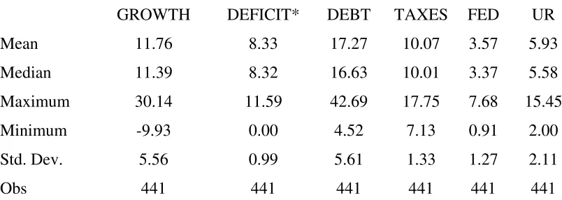
Table (1) reports summary statistics for the five-year-interval data used to estimate equation
8
range from zero to ten and have an average and median of about 8 and a standard deviation of
about 3.
V. ESTIMATES
We begin with ordinary least-squares (OLS) estimates as our baseline estimates eq. (1).
OLS estimates are reported in Table (2) for a lag of 2 periods (ten years), one period prior to the
base year for growth, which yields a strictly recursive structure.
The R-squared of 0.61 in Table 2 is respectably large for a five-year growth interval, and
the coefficient for the ACIIR-debt interaction (3.9) is significantly positive at the five percent
level, consistent with the WW argument that BBRs increase growth by increasing the productive
effect of debt by restricting public borrowing to investments in productive infrastructure.
Coefficients for all other fiscal variables are insignificant at p<.05 at this long-lag interval,
although lagged DEBT is significantly negative at p<.10. Carlino and Inman (2013) and Eberts
and Stone (1992) also report insignificant effects for similarly long horizons. In this context, the
significance of the ACIR-debt interaction is striking. Note, again, that ACIR cannot be included
independently because it contains no variation independent from state and period fixed effects,
so any direct effects of the ACIR index if any, are captured by the fixed effects. We turn next to
the issue of whether the coefficient for the interaction is identified by endogenous or exogenous
variation and then to issues of robustness and placebo regressions.
V.1 Exogeneity
To perform a standard Hausman test of the null hypothesis of exogeneity, we rely on
three-period lagged values of the independent variables as instruments for the ACIR-debt interaction.
That is, we use the ACIR-debt interaction lagged fifteen years and similarly lagged values of the
9
0.83 and an F statistic of 32, well above the Stock-Yogo (2001) critical value for the null
hypothesis of weak instruments.3 Results for the Hausman test are reported in Table (3), where
the p value for the coefficient for the first-stage residual (H-TEST) fails to reject the null
hypothesis of exogeneity for the ACIR-debt interaction at the five percent level. Even so, we
also report estimates based on the two-step, generalized method of moments (GMM) estimator in
Table (4). The coefficient for the interaction term is significantly positive and rises
insignificantly (based on the Hausman test) from the OLS estimate of 3.9 to 4.5; the Hansen’s J
statistic of 27.3 fails to reject exogeneity for the instruments at the five percent level;4 the null
hypothesis for an insignificant AR2 is not rejected; and the coefficient for lagged growth (-0.01)
in Table (4) is notably small and insignificant. We have no reason thus far, to abandon the OLS
estimates in Table (2), so we take the OLS estimate of 3.9 as our preferred estimate and report
the GMM estimates in Table (4) merely for comparison.
V.2 Robustness
The OLS results in Table (2) are qualitatively invariant to several alternative specifications,
including the addition of controls for the age composition of the population5 or the addition of
PROD, the lagged state income share invested in productive public infrastructure. The latter
suggests that the coefficient for the ACIR-debt interaction is not significantly influenced by
cyclical investments in public infrastructure. What aspect of the specification is not robust?
Shortening the lag interval from two periods to only one (from ten to five years) disrupts the
3
Individual unit roots are rejected for all variables.
4
(Chi-square/37-17/.05= 31.4).
5
(percent of population 5-17, 18-64, and the implicit remainder for younger than 5 or older than
10
strictly recursive structure and yields an insignificant coefficient of (3.0) for the ACIR-DEBT
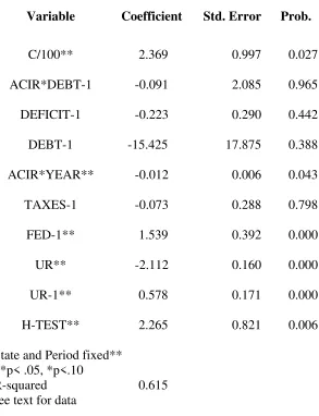
interaction in Table (5). Not surprisingly, results in Table (6) for a Hausman test for the one-lag
specification identified analogously to the longer two-period lag specification that is, with
independent variables lagged j+1 (two) periods as instruments reject exogeneity at the five
percent level at this shorter lag. Evidence that single-lagged values are endogenous is a useful
finding, given that previously published studies have relied on single-period lags for
identification. The two-period lag specification appears superior even for the five-year intervals.
In light of the endogeneity present in the one-lag specification, we present GMM estimates for
the one-period lagged specification with two-period lagged instruments. Table (7) reports these
estimates, and the ACIR-debt coefficient is again significantly positive at (3.3). Unlike the
two-lag GMM specification based on three-period two-lagged instruments, the one-period two-lag GMM
coefficient for lagged growth in Table (7) is significantly positive at (0.19). Even so, an
insignificant AR2 is not rejected, and the Hansen J-statistic of 27.3 fails to reject the null
hypothesis of exogeneity for the instruments.6 All estimates in Tables 2 through 7 for which
exogeneity is not rejected yield a significantly positive coefficient for the ACIR-debt interaction,
regardless of specification or estimator. The median across the range of these estimates (3.3 to
4.5) is 3.9, which coincides with the OLS estimate for the two-lag strictly recursive,
specification—our preferred specification. We now turn to placebo regressions as another form
of robustness check.
V.3 Placebo regressions
Placebo regressions are useful as a test for whether or not an effect is spurious because it is
present where it should not be. An expedient choice for a placebo regression in the present
6
11
context is to test whether the ACIR-debt interaction in one region has a significant effect in other
regions, even though it should not, unless region spillovers are important. To test whether the
ACIR-debt interaction in any of the nine Census regions has a significant effect on growth of
other regions, we regress growth across all states in turn, on the ACIR-DEBT variable for each
of the nine Census regions. Note that these placebo regressions are not a test for the general
significance of regional spillovers from one specific region to another individual region. Instead,
they are a test of whether regional spillovers or other factors spuriously common to states are
responsible for the positive estimate for the effect of the ACIR-debt interaction in Table (2).
Placebo regressions in this context are expediently conservative in the sense that regional
spillovers will bias results toward a false placebo effect. Even so, we find no significantly
positive effect for the ACIR-debt interaction in any of the nine regressions. To illustrate the
results of the nine placebo regressions in a compact form, Table (8) presents results for the
ACIR-DEBT interaction for Census region 4, which closely coincide with the median result
across the nine placebo regressions. The next robustness check is to gauge the sensitivity of the
results to outlying observations.
V.4 Outliers
To address the issue of sensitivity to outlying observations, residuals that are more than two
standard deviations above or below the regression norm are identified, and dummy variables
identifying these observations are added to the primary regression specification. Results from
this augmented regression are equivalent and the correlations between the outlier residuals and
the two key variables, growth and ACIR*DEBT are insignificant. The final robustness check is
to determine the sensitivity of the standard errors to alternative correction procedures.
12
We explore the sensitivity of the standard errors by obtaining state-specific residual variances
and period-specific residual variances from the OLS residuals from the specification in Table 2,
including both state and period fixed effects. The variance across the state-specific residuals is
3.43, and the variance across the period-specific residuals is 3.59. The ratio of the latter to the
former is 1.06, indicating slightly greater dispersion across periods than across states, which is
why Table (2) reports period-weight panel corrected standard errors (PCSEs). If cross-section
weight PCSEs are used instead, results are equivalent. The cross-section weight PCSE for the
ACIR–DEBT coefficient is (2.12). We also calculate the period SUR (PCSE) for the
ACIR-DEBT coefficient, and again the results are equivalent. The period SUR PCSE is (2.03).
VI. DISCUSSION
Given the regression estimates in Table (2), we are now in a position to discuss whether
or not BBRs change the effect of debt on growth, and if so, how. The significantly positive
coefficient for the ACIR-debt interaction suggests that the answer to the first question is ‘yes’:
more stringent BBRs make debt more productive, consistent with the WW view that these rules
increase the productiveness of debt by restricting borrowing to productive public infrastructure.
This effect could work either directly through the greater productivity of investments in public
infrastructure or more indirectly by assuring lenders that future borrowing will be limited to
public infrastructure, resulting in lower costs of borrowing. Both channels are consistent with
the evidence in Alt and Lowry (1997) and others that borrowing costs are lower for states with
more stringent budget rules.
How large is the effect of BBRs on the productivity of debt in terms of growth? With no
BBR in place (i.e., with an ACIR index of zero) and evaluated at sample means, the coefficients
13
5.6 percent of personal income) decreases the steady-state (five-year) growth rate by 17.4
percent of real income—just over 3 percent per year. However, with a strict BBR in place (i.e.,
with an ACIR index of 10), the coefficients predict instead an increase in the steady-state
(five-year) growth rate of about 15 percent for a one-standard-deviation increase in debt.
VII. POLICY CONSIDERATIONS
Evidence elsewhere indicates that balanced-budget rules lower borrowing costs and
restrain levels of state and local debt. Our evidence also indicates that high levels of debt can
slow growth, but our unique contribution is to provide an arguably well-identified test of the
hypothesis that state-level balanced-budget restrictions in the U. S. increase growth by restricting
borrowing to productive public infrastructure. Evidence that state balanced-budget restrictions
increase growth via this channel provides the first formal test of the WW hypothesis and adds a
new perspective to the effects of balanced-budget rules by suggesting that the benefits of tax
smoothing and fiscal flexibility (permitted in the absence of a balanced-budget restriction) may
come at the expense of lower growth. We close however, with caveats; we provide evidence
relevant to the WW hypothesis, not a comprehensive analysis of the merits of balanced-budget
and other fiscal restrictions. In particular, the context for fiscal policy differs in obvious and
important ways for countries and sub-national states. Auerbach (2007) for example, analyzes
14
REFERENCES
Adam, C. S. and Bevan, D. L. (2005). “Fiscal Deficits and Growth in Developing Countries.”
Journal of Public Economics, 89: 571-597.
Advisory Commission on Intergovernmental Relations. 1987. Fiscal Discipline in the Federal
System: national reform and the experience of the states. Washington, DC: ACIR.
Ash, M. Herndon, T. and Robert Pollin (2013). ‘Does High Public Debt Consistently Stifle
Economic Growth? A Critique of Reinhart and Rogoff’ working paper, U. Mass.
Alesina, A, and Bayoumi, T. (2006). “The Costs and Benefits of Fiscal Rules: Evidence From
U.S. States,” NBER working paper.
Auerbach, A. J. (2000). “Formation of Fiscal Policy: The Experience of the Past Twenty-Five
Years”, Federal Reserve Bank of New York Economic Policy Review, April, 1-15.
Bania, N., Gray, J. A. and Stone, J. A. 2007. “Growth, Taxes, and Government Expenditures:
Growth Hills for U.S. states,” National Tax Journal, 60:193-204.
Barro, R. J. (1989). “Government Spending in a Simple Model of Endogenous Growth,”
Journal of Political Economy, 98: S103-26.
Bleaney, M., Gemmell, N., and Kneller, R. (2001). “Testing the Endogenous Growth Model:
Public expenditure, taxation, and growth over the long run,” Canadian Journal of
Economics, 34: 36-57.
Carlino, G. and R. Inman (2013). “Local Deficits and Local Jobs: Can States Stabilize Their
Own Economies? NBER working paper number 18930.
Checherita-Westphal, C., A.H. Hallett and P. Rother (2012) “Fiscal Sustainability using
15
Eberts, R. W. and J. A. Stone (1992). Wage and Employment Dynamics in Urban Labor
Markets, Kalamazoo: W.E. Upjohn Institute for Employment Research.
Gray, J. and J. Stone (2012). “Nonlinearities in the Effects of Debt and Fiscal Policy: Evidence
from the States,” Economic Research Guardian 2:2: 152-159.
Greiner A. and B Fincke (2012) Public Debt and Economic Growth, Berlin and Heidelberg:
Springer-Verlag Press.
Greiner, A. (2013)”Debt and growth: Is There a Non-Monotonic Relation?” Economics Bulletin,
33: 340-47.
Krol, R. and S. Svorny (2007). “Budget Rules and State Business Cycles,” Public Finance
Review, 35: 530-544.
Poterba, J. and K. Reuben. eds. (1999). Fiscal Institutions and Fiscal Performance: U. Chicago.
Bohn, H. and R. Inman (1995). “Constitutional Limits and Public Deficits: Evidence From the
U.S. States,” Carnegie-Rochester Conference Series on Public Policy, 45: 3-76.
Capeci, J. (1994). “Local Fiscal Policies, Default Risk, and Municipal Borrowing Costs,”
Journal of Public Economics, 53: 73-89.
Inman, R. (1996). “Do Balanced Budget Rules Work? U.S. Experience and Possible Lessons
for the EMU,” NBER Working Paper no. 5838.
Levinson, A. (1997. “Balanced Budgets and Business Cycles: Evidence from the States,” Dept.
of Economics, U. Wisconsin, photocopy.
Lowry, R. and J. Alt. 1997). “A Visible Hand? Bond markets, Political Parties, Balanced
Budget Laws, and State Government Debt,” Dept. of Government, Harvard, photocopy.
Mofidi, Ala and Joe Stone (1990). “Do State and Local Taxes Affect Economic Growth?” The
16
Poterba, J. (1989). “Tax Reform and the Market for Tax-Exempt Debt,” Regional Science and
Urban Economics, 195: 37-62.
Poterba, J. (1994). “State Responses to Fiscal Crises: The Effects of Budgetary Institutions and
Politics,” Journal of Political Economy, 102: 799-8.
Reed, R. (2008). ‘The Robust Relationship between Taxes and U. S. State Income Growth,’
National Tax Journal, 61:5-80.
Reinhart, C. and K. Rogoff (2010). Growth in a Time of Debt. American Economic Review,
100, 2: 573-8.
Wallis, J. and B. Weingast (2009). “Dysfunctional or Optimal Institutions? State Debt
Limitations, the Structure of State and Local Governments and the Finance of American
Infrastructure” in Fiscal Challenges: An Interdisciplinary Approach, Elizabeth Garrett,
17
TABLE 1 Summary Statistics (49 states 1957-2007)
GROWTH DEFICIT* DEBT TAXES FED UR
Mean 11.76 8.33 17.27 10.07 3.57 5.93
Median 11.39 8.32 16.63 10.01 3.37 5.58
Maximum 30.14 11.59 42.69 17.75 7.68 15.45
Minimum -9.93 0.00 4.52 7.13 0.91 2.00
Std. Dev. 5.56 0.99 5.61 1.33 1.27 2.11
Obs 441 441 441 441 441 441
GROWTH is the log change in real personal income per capita (five-year intervals).
Fiscal data are percentage points of state personal income. See text for data.
18
TABLE 2 Two-Lag OLS Growth Estimates
49 states 1957-2007 no. obs. 391)
(period weight PCSEs)
Variable Coeff Std. Error Prob.
C/100** 2.740 0.861 0.000
DEFICIT-2 0.226 0.256 0.378
DEBT-2* -20.406 10.727 0.058 ACIR*DEBT-2** 3.878 1.230 0.002 ACIR*YEAR** -0.014 0.004 0.001 TAXES-2 0.106 0.340 0.755 FED-2 0.209 0.529 0.692 UR** -2.105 0.234 0.000 UR-2** 0.459 0.126 0.003 State and period fixed**
R-squared 0.611 **p< .05 *p<.10
19
TABLE 3 Hausman Test, Two-Lag Estimates
(no. obs. 391)
(period weight PCSEs)
Variable Coefficient Std. Error Prob.
C/100** 2.52 1.05 0.02
DEFICIT-2 0.01 0.30 0.97
DEBT-2 -9.61 18.41 0.60
ACIR*DEBT-2* 3.84 2.26 0.09
ACIR*YEAR** -0.01 .001 0.02
TAXES-2 0.38 0.29 0.19
FED-2 0.45 0.40 0.26
UR** -2.08 0.17 0.00
UR-2* 0.28 0.16 0.09
H-TEST* -2.25 1.29 0.08 State fixed**
Period fixed**
R-squared 0.58 ** p<.05, * p<.10
See text for data
20
TABLE 4 Two-Lag GMM Growth Estimates
Notes: **p<.05 *p<.10
See text for data
(No.obs. 391)
White period instrument weighting matrix (White-period std.err.)
Variable Coefficient Std. Error
Prob.
GROWTH-1) -0.013 0.042 0.743 DEFICIT-2) 0.138 0.148 0.353 DEBT-2)** -26.361 7.134 0.000 ACIR*DEBT-2)** 4.535 0.898 0.000 TAXES-2) 0.086 0.141 0.540 ACIR*YEAR** -0.013 0.002 0.000 FED-2)** 0.396 0.254 0.119 UR** -1.936 0.125 0.000 UR-2)** 0.478 0.081 0.000 State and Period fixed**
R-squared 0.522
AR2 (p=0.433)
21
TABLE 5 One-Lag OLS Growth Estimates
(No. obs. 489)
(period weight PCSEs)
Variable Coefficient Std. Error Prob.
C/100** 2.945 84.133 0.005
ACIR*DEBT-1 2.976 1.927 0.123
DEFICIT-1 -0.069 0.285 0.806
DEBT-1 -30.583 16.918 0.071
ACIR*YEAR** -0.013 0.005 0.009
TAXES-1 0.291 0.264 0.272
FED-1** 0.994 0.364 0.006
UR** -2.070 0.160 0.000
UR-1** 0.662 0.159 0.000
Cross-section fixed**
Period fixed**
R-squared 0.583
**p<.05 *p<.10
See text for data
22
TABLE 6 Hausman Test One-Lag Estimates
(No. obs. 391)
(period weight PCSEs)
Variable Coefficient Std. Error Prob.
C/100** 2.369 0.997 0.027
ACIR*DEBT-1 -0.091 2.085 0.965
DEFICIT-1 -0.223 0.290 0.442
DEBT-1 -15.425 17.875 0.388
ACIR*YEAR** -0.012 0.006 0.043
TAXES-1 -0.073 0.288 0.798
FED-1** 1.539 0.392 0.000
UR** -2.112 0.160 0.000
UR-1** 0.578 0.171 0.000
H-TEST** 2.265 0.821 0.006
State and Period fixed** **p< .05, *p<.10
23
TABLE 7 One-Lag GMM Growth Estimates
(No. obs.489) period weight instrument matrix) White-period standard errors)
Variable Coefficient Std. Error Prob.
GROWTH-1** 0.199 0.062 0.001
DEFICIT-1 0.114 0.363 0.752
DEBT-1 -14.390 13.498 0.287
ACIR*DEBT-1** 3.273 1.526 0.032
ACIR*YEAR** -0.009 0.002 0.000
TAXES-1** -0.734 0.258 0.004
FED-1** 1.890 0.213 0.000
UR** -2.107 0.114 0.000
UR-1** 1.141 0.246 0.000
State and Period fixed**
**p< .05. *p<.10 See text for data.
24
TABLE 8 Placebo Regressions: Median Result for Census Regions (Census Region 4)
Dependent Variable: GROWTHREG4 Total panel (unbalanced) observations: 440 White-period standard errors)
Variable Coefficient Std. Error Prob.
C/100** 0.767 0.385677 0.0470
ACIR*DEBT-2 0.320 0.540276 0.5538
DEFICIT-2 0.171 0.140513 0.2231
DEBT-2 -3.881 4.266604 0.3635
ACIR*YEAR* -0.004 0.002400 0.0568
FED-2 0.228 0.168553 0.1760
UR 0.032 0.044967 0.4749
UR-2 0.053 0.086337 0.5395
TAXES-2 -0.216 0.251445 0.3907
Cross-section fixed**
Period fixed** R-squared
**sig at .05 see text for data and variables.
0.846