S Bandyopadhyay, D S Sharma and R Sangal. Proc. of the 14th Intl. Conference on Natural Language Processing, pages 466–475, Kolkata, India. December 2017. c2016 NLP Association of India (NLPAI)
Open Set Text Classification using Convolutional Neural Networks
Sridhama Prakhya†, Vinodini Venkataram‡and Jugal Kalita‡
†School of Engineering & Technology, BML Munjal University, Gurugram, India ‡Department of Computer Science, University of Colorado Colorado Springs, USA
†[email protected] ‡{vvenkata,jkalita}@uccs.edu
Abstract
In a closed world setting, classifiers are trained on examples from a number of classes and tested with unseen examples belonging to the same set of classes. However, in most real-world scenarios, a trained classifier is likely to come across novel examples that do not belong to any of the known classes. Such examples should ideally be categorized as belonging to an unknown class. The goal of anopen set classifier is to anticipate and be ready to handle test examples of classes unseen during training. The classifier should be able to declare that a test example belongs to a class it does not know, and possi-bly, incorporate it into its knowledge as an example of a new class it has encoun-tered. There is some published research in open world image classification, but open set text classification remains mostly un-explored. In this paper, we investigate the suitability of Convolutional Neural Net-works (CNNs) for open set text classifi-cation. We find that CNNs are good fea-ture extractors and hence perform better than existing state-of-the-art open set clas-sifiers in smaller domains, although their open set classification abilities in general still need to be investigated.
1 Introduction
With increasing amounts of textual data being gen-erated by various online sources like social net-works, text classifiers are essential for the anal-ysis and organization of data. Text classification usually consists of training a classifier on a la-beled text corpus where individual examples be-long to one or more classes based on their
In the recent past, many-layered Artificial Neu-ral Networks (ANN) or deep learning techniques (Goodfellow et al., 2016) have become popular in Computer Vision and Natural Language Process-ing. This is mainly attributed to the increase in performance compared to standard machine learn-ing techniques. As discussed later, current open set text classifiers do not rely on deep learning models. They employ either a clustering-based ap-proach (Doan and Kalita, 2017) or a modified Sup-port Vector Machine (SVM) (Fei and Liu, 2016). To this end, we explore the possibility of using a CNN for open set text classification and compare it to existing techniques.
2 Related Work
To allow for the possibility that the set of classes is open or expandable during deployment, the classi-fication algorithms need to be adaptive. (Scheirer et al., 2013) combine empirical risk and open space risk due to the existence of a space in which classification probabilities are not currently known. Empirical risk comes from actual ex-amples being misclassified by a trained classifier, and the open space risk recognizes the fact that the presence of unknown classes is likely to in-troduce errors into classification decisions. Their model reduces the risk by introducing parallel hy-perplanes, one near the class boundary and an-other far from it to introduce slabs of subspaces for the classes, and then develops a greedy op-timization algorithm that modifies a linear SVM and moves the planes incrementally. This work was extended to multi-class open set classification by introducing what (Scheirer et al., 2014) call a Compact Abating Probability (CAP) model. They build a classifier called W-SVM using properties of Extreme Value Theory for calibration of scores produced by 1-class and binary SVMs. Extreme Value Theory (EVT) (Smith, 1990; De Haan and Ferreira, 2007; Castillo, 2012) is usually used to deal with and predict rare events or values that oc-cur at the tails of distributions. The unnormalized probability of inclusion for each class is estimated by fitting a Weibull distribution (Sharif and Islam, 1980) over the positive class scores from SVM classifiers. The assumption here is when a trained classifier cannot classify an example as belonging to any of the known classes, it is a case of “fail-ure” of the classifier and is deemed unusual. (Jain et al., 2014) also use EVT to formulate the open
set classification problem as one of modeling pos-itive training data at the decision boundary. They introduce a new algorithm called the Pi-SVM for estimating the unnormalized posterior probability of class inclusion. Their approach is different from the one introduced by (Platt and others, 1999) of taking SVM outputs and converting them to prob-abilities by fitting a sigmoid function to the SVM scores.
(Bendale and Boult, 2015) present an approach to minimize the weighted sum of empirical risk and open set risk using thresholding sums of monotonically decreasing recognition functions, and use their approach to extend the Nearest Cen-troid Classifier (NCM) (Rocchio, 1971). This classifier represents classes by the mean feature vector of its elements. An unseen example is as-signed a class with the closest mean. The Near-est Non-Outlier (NNO) algorithm (Bendale and Boult, 2015) adapts NCM for open set classifica-tion, taking into account open space risk and met-ric learning. The nearest class mean metmet-ric learn-ing (NCMML) (Mensink et al., 2013) approach extends the NCM technique by replacing the Eu-clidean distance with a learned low-rank Maha-lanobis distance. This gives better results than the former as the algorithm is able to learn features inherent in the training data.
All the work mentioned so far have been in the context of computer vision. Work in open set clas-sification for textual data is limited. (Fei and Liu, 2016) use CBS learning (Fei and Liu, 2015) where a document is represented as a vector of similari-ties from centers of spheres that correspond to in-dividual classes. Around the sphere that represents positive examples of a class, they draw a slightly bigger sphere to provide additional space for a class to accommodate unseen examples. They also use SVM hyperplanes to bound the bigger spheres. The unbounded regions correspond to unknown classes.
The Nearest Centroid Class (NCC) algorithm (Doan and Kalita, 2017) builds upon the NCM, but uses a density-based method following the approach of the clustering algorithm called DB-SCAN (Ester et al., 1996). They represent a class not by a sphere but a set of density-connected gions and also consider the centroids of these re-gions and not the means.
2012) to perform open set classification in the vi-sion domain. In closed set classification, the final softmax layer of the CNN essentially chooses the output class with the highest probability with re-spect to all other output labels. Bendale and Boult propose OpenMax, which is a new model layer that estimates the probability of an input belong-ing to an unknown class instead of softmax. (Ge et al., 2017) adapt OpenMax to generative adver-sarial networks (GANs) for open set vision prob-lems. There have been no such attempts in the text processing domain.
3 Method
Along the lines of existing open set techniques, our work was also motivated by the Rocchio method (Rocchio, 1971). We wanted to use pre-trained word vectors (Mikolov et al., 2013) for open set determination. This led us to perform experiments to see whether simple cosine com-putation can be used for open set classification. We used a naive approach to construct document vectors by averaging all word vectors (Le and Mikolov, 2014) in a document. We calculated the cosine similarities between the mean of all docu-ment vectors and a test example. Due to the sim-ilarities being too close (sometimes overlapping), we concluded that calculating cosine similarity at the document level was not suitable for open set classification.
Prior open set text classification models (CBS learning and NCC) do not use artificial neural net-works. We decided to pursue a novel approach to open set text classification that relied on a deep learning model, viz. CNNs due to their ability of extracting useful features. Since (Bendale and Boult, 2016) explored the use of CNNs in open set image classification, we started with their ap-proach as the basis and extend the work as nec-essary. The work of (Kim, 2014) in CNNs for sentence classification helped us arrive at an ef-ficient neural network architecture. Thus, we per-form experiments with a single-layer CNN, using the Weibull-modified final layer instead of soft-max. We also examine if increasing the number of CNN layers changes performance of open set text classification. We develop a novel ensemble approach to deal with the activations of the penul-timate layer of the CNN. The penulpenul-timate layer is the focus because this is the layer that contains the real activations for nodes corresponding to the
var-ious classes for the problem at hand. Since these are raw activations, in a standard CNN, they are converted into probability-like values by perform-ing the softmax operation.
sof tmax(x)i = Pexi
jexj
(1)
However, in our case, there is an unknown class to be considered as well and we do not know the activations or probabilities associated with such an unknown class. Therefore, this softmax layer needs to be modified. (Bendale and Boult, 2016) replace the layer that computes softmax with the so-called OpenMax layer, which uses a learned distance metric taking into account the open set risk.
Our new model uses an ensemble approach to make a decision with the activations in the penul-timate layer. Our model is also incremental in na-ture. This means, the model does not have to be retrained after the introduction of a new unknown class. This is because open set determination hap-pens after training, rather than during or before.
In our experiments discussed here, we compare the performance of our ensemble-based open set text classifier with other open set classifiers that have been previously used for image classification and the methods of (Fei and Liu, 2016) and (Doan and Kalita, 2017), which were used for open set text classification.
3.1 Datasets
For efficacious open world evaluation, we must choose a dataset with a large number of classes. This allows us to hide classes during training. These hidden classes can later be used during test-ing to gauge the open world accuracy. We use the following two freely available datasets.
• 20 Newsgroups (McCallum et al., 1998; Slonim and Tishby, 2000) - Consists of 18,828 documents partitioned (nearly) evenly across 20 mutually exclusive classes.
• Amazon Product Reviews(Jindal and Liu, 2008) - Consists of 50 classes of products or domains, each with 1,000 review documents. 3.2 Evaluation Procedure
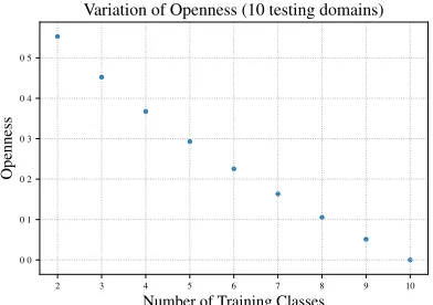
the model was trained on. In open set evaluation, the classifier has incomplete knowledge during the training phase. Examples of unknown classes can be submitted to the classifier during the testing phase. During the training phase, we train the classifiers on a limited number of classes. While testing, we then present the model with additional classes that were not learned during training. We evaluate the performance of the classifier based on how well it identifies these new classes. “Open-ness”, proposed by (Scheirer et al., 2013; Scheirer et al., 2014), is a measure to estimate the open world range of a classifier. This measure is only concerned with the number of classes rather than the open space itself.
openness= 1−p(2×CT)/(CR+CE) (2)
where:
CT =number of classes used for training
CR=number of classes to be recognized
CE =number of classes used during
evaluation/testing
As a special case, whenCT = CR = CE, the
value ofopennessis 0, i.e., it is the case of tradi-tional classification when the numbers of classes trained on, tested on, and recognized are the same. Accuracy, precision, recall, and F-score are used to measure the closed set performance of our model. These metrics are expanded to the open set scenario by grouping all unknown classes into the same subset. A True Positive is when an exam-ple of a known class is correctly classified and a True Negative is when an example of an unknown class is correctly predicted as unknown. False Pos-itives (an unknown class predicted as known) and False Negatives (a known class predicted as un-known) are the two types of incorrect class assign-ment. Figure 1 shows howopenness varies with the number of training classes when there are 10 testing classes.
4 Experiments
For all experiments, the CNN-static architecture proposed by (Kim, 2014) is used. We use pre-trained word2vec1 (Mikolov et al., 2013) vec-tors as our word embeddings. These embeddings are kept static while other parameters of the model
1https://code.google.com/p/word2vec/
2 3 4 5 6 7 8 9 10
Number of Training Classes
0.0 0.1 0.2 0.3 0.4 0.5
Openness
[image:4.612.326.522.46.184.2]Variation of Openness (10 testing domains)
Figure 1: Variation of openness with number of training classes
Table 1: CNN baseline configuration
Description Values
word embedding word2vec
filter sizes (3,4,5)
feature maps 100
activation function ReLU
pooling 1-max pooling
dropout rate 0.5 L2norm constraint 0.0
are learned. According to the experiments of (Zhang and Wallace, 2015), imposing anL2norm constraint on the weight vectors generally does not improve performance drastically. Figures 3 and 4 show the accuracies achieved on the 20 News-groups dataset while varying the L2 norm con-straint. Increasing theL2 norm constraint proved
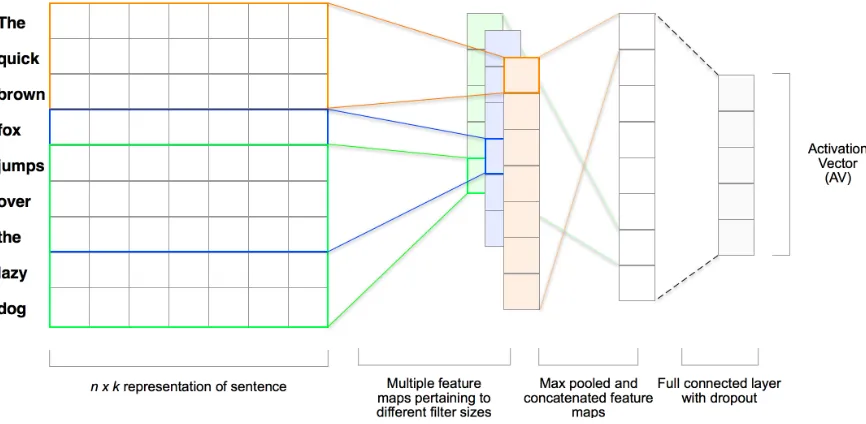
detrimental to the model accuracy. The configura-tion details of the CNN used in all our experiments are shown in Table 1. Figure 2 shows a depiction of the CNN architecture we implemented. In our case, we use a single static channel instead of mul-tiple channels.
4.1 Multi-layer CNN
In addition to Kim’s architecture, we have also ex-perimented with multi-layer CNNs. We used 2 convolutional layers, the initial layer used a ker-nel of size 3×1, while the second layer used a
kernel of size 3×300. The first layer convolves
[image:4.612.317.533.265.378.2]Figure 2: Model architecture with multiple filter sizes (3, 4, 5) for an example sentence
Figure 3: L2 constraint = 0.0, Model Accuracy: 0.710
Figure 4: L2 constraint = 3.0, Model Accuracy: 0.672
tors from the antepenultimate layer, which may represent the document more accurately. Unfor-tunately, the closed set (trained on 3 classes) accu-racy of the muli-layer CNN was around 75%. The accuracy decreased significantly as we increased the number of training classes. A high closed set accuracy is necessary to achieve respectable open set results. Intuitively, the model must have a com-prehensive understanding of what it knows. Only
then can it be competent enough to classify un-known inputs correctly.
4.2 Ensemble Approach
In our open set classifier, we use an ensemble of approaches to determine whether a test example is from a known class or not. This ensemble in-cludes probabilistic and high dimensional outlier detectors.
4.2.1 Isolation Forest
The isolation forest algorithm (Liu et al., 2008) de-tects outliers using combinations of a set of iso-lation trees. Isoiso-lation trees recursively partition the data at random partition points with randomly chosen features. Doing so isolates instances into nodes containing only one instance. The heights of branches containing outliers are comparatively less than other data points. The height of the branch is used as the outlier score. The scores ob-tained from the isolation forest are min-max nor-malized and calculated for every training class. Examples with scores below a predefined thresh-old are labelled as unknown. In case of multi-ple scores above the threshold, the exammulti-ple is as-signed to the class with the highest score.
4.2.2 Probabilistic Approach
[image:5.612.81.302.452.555.2]network. We call these scores activation vectors (AV). We deviate from the original OpenMax by finding thek-nearest examples to the centroid of every training class. We refer to these examples as k-Class Activation Vectors (k-CAV). For ev-ery example in a training class, we calculate the distances between the respective AV and the k-CAVs. Doing so, results in k distances per AV. We then take the average of thesekcalculated dis-tances. As the number of classes in our dataset is far less than those used in image classification, the k-CAVs of a class are used represent a class more accurately than a single mean activation vec-tor. This also mitigates the effect of outlier AVs in a class. We observed that whenk is around 10, the trade-off between performance and computa-tion time is optimized. Therefore, for all experi-ments, we fix the value ofk= 10.
In our outlier ensemble, we use two distance metrics – Mahalanobis distance and Euclidean-cosine (Eucos) distance (Bendale and Boult, 2016). Ideally, we want a distance metric that can tell us how much an example deviates from the class mean. The Mahalanobis distance precisely does this by giving us a multi-dimensional gener-alization of the number of standard deviations a point is from the distribution’s mean. The closer an example is to the distribution mean, the lower is the Mahalanobis distance. The Mahalanobis dis-tance between point x and point y is given by:
d(~x, ~y) = q
(~x−~y)TC−1(~x−~y) (3)
whereCis the covariance matrix, among the fea-ture variables calculated a priori. The Euclidean-cosine distance is a weighted combination of Eu-clidean and cosine distances.
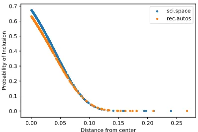
The distances obtained are used to generate a Weibull model for every training class. We use the libMR2(Scheirer et al., 2011)FitHighmethod
to fit these distances to a Weibull model that re-turns a probability of inclusion of the respective class. Figure 5 shows the probabilities of inclusion obtained from the generated Weibull model for 2 training classes belonging to the 20 Newsgroups dataset. As an example deviates more from the class center (k-CAVs), the probability of inclusion decreases.
The sum of all inclusion probabilities is taken as the total closed set probability. Open set prob-ability (OSP) is computed by subtracting the total
2https://github.com/Vastlab/libMR
0.00 0.05 0.10 0.15 0.20 0.25 Distance from center
0.0 0.1 0.2 0.3 0.4 0.5 0.6 0.7
Probability of Inclusion
sci.space rec.autos
Figure 5: Weibull distribution generated using libMR for two classes belonging to the 20 News-groups dataset
closed set probability from 1.
OSP = 1−total closed set probability (4)
[image:6.612.323.522.52.185.2]We then compare the maximum closed set prob-ability and total open set probprob-ability. If the total open set probability is greater than the former, we label the example as unknown, otherwise, the ex-ample is assigned the class with the highest closed set probability. Parameters like threshold and dis-tribution tail-size can be be adjusted to decrease the open-space risk.
Figure 6: Our ensemble model
We use a voting scheme to combine the three approaches (Mahalanobis Weibull, Eucos Weibull and Isolation Forest), see Figure 6. It has been observed that Mahalanobis and Eucos perform nearly the same. Predictions from the Isolation Forest are usually used as a tie-breaker in case of differing predictions. When all 3 predictions dif-fer, we give the Eucos Weibull the highest priority.
5 Results and Discussion
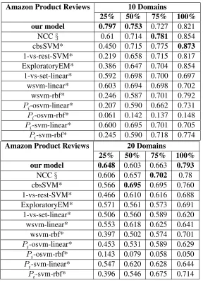
[image:6.612.314.544.418.515.2]Table 2: Experiments on Amazon Product Reviews dataset (10, 20 domains)
Amazon Product Reviews 10 Domains
25% 50% 75% 100%
our model 0.797 0.753 0.727 0.821
NCC§ 0.61 0.714 0.781 0.854
cbsSVM* 0.450 0.715 0.775 0.873
1-vs-rest-SVM* 0.219 0.658 0.715 0.817
ExploratoryEM* 0.386 0.647 0.704 0.854
1-vs-set-linear* 0.592 0.698 0.700 0.697
wsvm-linear* 0.603 0.694 0.698 0.702
wsvm-rbf* 0.246 0.587 0.701 0.792
Pi-osvm-linear* 0.207 0.590 0.662 0.731
Pi-osvm-rbf* 0.061 0.142 0.137 0.148
Pi-svm-linear* 0.600 0.695 0.701 0.705
Pi-svm-rbf* 0.245 0.590 0.718 0.774
Amazon Product Reviews 20 Domains
25% 50% 75% 100%
our model 0.648 0.603 0.663 0.793
NCC§ 0.606 0.657 0.702 0.78
cbsSVM* 0.566 0.695 0.695 0.760
1-vs-rest-SVM* 0.466 0.610 0.616 0.688
ExploratoryEM* 0.571 0.561 0.573 0.691
1-vs-set-linear* 0.506 0.560 0.589 0.620
wsvm-linear* 0.553 0.618 0.625 0.641
wsvm-rbf* 0.397 0.502 0.574 0.701
Pi-osvm-linear* 0.453 0.531 0.589 0.629
Pi-osvm-rbf* 0.143 0.079 0.058 0.050
Pi-svm-linear* 0.547 0.620 0.628 0.644
Pi-svm-rbf* 0.396 0.546 0.675 0.714
usually overlap in vector space. Similar to (Fei and Liu, 2016; Doan and Kalita, 2017), we conduct our experiments by introducing “unseen” classes during testing. In reality, as the train-test partition can be random, we arbitrarily specify the number of testing domains. For every domain, we report our results using 5 random train-test partitions for each dataset. Both datasets are evaluated on the same number of test classes (10, 20). We also eval-uate our model on smaller domains, shown in Ta-ble 4. The number of testing classes used during training is varied in quarter-step increments (25%, 50%, 75% and 100%). We take the floor value in case of fractional percentages. Using 100% of the testing classes during training corresponds to closed set classification.
Results of the Amazon Product Reviews and 20 Newsgroups datasets are shown in Tables 2 and 3 respectively. We report only the F-scores due to
space constraints. Classifiers used as baselines for comparison are described below.
• 1-vs-rest-SVM - Standard 1-vs-rest multi-class SVM with Platt Probability Estimation (Platt and others, 1999)
• 1-vs-set-linear - 1-vs-set machine model proposed by (Scheirer et al., 2013)
• W-SVM- Weibull-calibrated SVM (Scheirer et al., 2014)
• Pi-SVM- SVM model that estimates the
un-normalized posterior probability of class in-clusion (Jain et al., 2014)
• ExploratoryEM - “Exploratory” version of Expectation-Maximization algorithm (EM) (Dalvi et al., 2013)
• cbsSVM - Center-Based Similarity Space SVM (Fei and Liu, 2016)
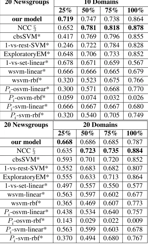
Table 3: Experiments on 20 Newsgroups dataset (10, 20 domains)
20 Newsgroups 10 Domains
25% 50% 75% 100%
our model 0.719 0.747 0.738 0.864
NCC§ 0.652 0.781 0.818 0.878
cbsSVM* 0.417 0.769 0.796 0.855
1-vs-rest-SVM* 0.246 0.722 0.784 0.828 ExploratoryEM* 0.648 0.706 0.733 0.852 1-vs-set-linear* 0.678 0.671 0.659 0.567
wsvm-linear* 0.666 0.666 0.665 0.679
wsvm-rbf* 0.320 0.523 0.675 0.766
Pi-osvm-linear* 0.300 0.571 0.668 0.770 Pi-osvm-rbf* 0.059 0.074 0.032 0.026 Pi-svm-linear* 0.666 0.667 0.667 0.680 Pi-svm-rbf* 0.320 0.540 0.705 0.749
20 Newsgroups 20 Domains
25% 50% 75% 100%
our model 0.668 0.686 0.685 0.787
NCC§ 0.635 0.723 0.735 0.884
cbsSVM* 0.593 0.701 0.720 0.852
1-vs-rest-SVM* 0.552 0.683 0.682 0.807 ExploratoryEM* 0.555 0.633 0.713 0.864 1-vs-set-linear* 0.497 0.557 0.550 0.577
wsvm-linear* 0.563 0.597 0.602 0.677
wsvm-rbf* 0.365 0.469 0.607 0.773
Pi-osvm-linear* 0.438 0.534 0.640 0.757 Pi-osvm-rbf* 0.143 0.029 0.022 0.009 Pi-svm-linear* 0.563 0.599 0.603 0.678 Pi-svm-rbf* 0.370 0.494 0.680 0.767
• NCC - Nearest Centroid Class model (Doan and Kalita, 2017)
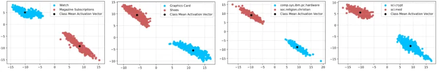
F-score performances of 1-vs-rest-SVM, 1-vs-set SVM, W-SVM,Pi-SVM, and cbsSVM are from study (Fei and Liu, 2016), marked as *. Re-sults pertaining to the Nearest Centroid Class model (NCC) are from study (Doan and Kalita, 2017), marked as §. Our model performs bet-ter than cbsSVM and NCC classifiers in smaller domains. Figure 7 shows the activation vectors obtained from models trained on 2 classes plot-ted in 2-dimensional space. The plots show dis-tinct clusters of activation vectors. We believe the CNN approach effectively isolates documents in smaller domains compared to other SVM-based approaches.
[image:8.612.316.531.518.591.2]Unlike cbsSVM, our model is an incremental model i.e., we do not have to retrain the model
Table 4: Open set results of Amazon Product Re-views Dataset in smaller domains (3, 4, 5)
Classes Trained on Classes Tested on
3 4 5
2 0.802 0.824 0.808
3 - 0.725 0.763
4 - - 0.797
when new unknown classes are introduced. Such models are more viable in real world scenarios.
6 Conclusion
Figure 7: Activation vectors obtained from models trained on 2 randomized classes.
classifying novel data, applications of which can be used to tackle tough text classification problems in domains like forensic linguistics.
Our future work will involve improving the number and diversity of classifiers used in the en-semble. In addition, we plan to consider different neural network architectures that learn sequential information from text, namely variants of recur-rent neural networkslikeLong Short-Term Mem-orynetworks withattentionmechanism.
Acknowledgments
This material is based upon work supported by the National Science Foundation under Grant Nos. IIS-1359275 and IIS-1659788. We are thankful for the support of BML Munjal University, partic-ularly Prof. Sudip Sanyal and Dr. Satyendr Singh. We also thank Diptodip Deb and Kyle Yee for their insightful discussions and constant encour-agement.
References
Abhijit Bendale and Terrance Boult. 2015. Towards
open world recognition. InProceedings of the IEEE
Conference on Computer Vision and Pattern Recog-nition, pages 1893–1902.
Abhijit Bendale and Terrance E Boult. 2016. Towards
open set deep networks. InProceedings of the IEEE
Conference on Computer Vision and Pattern Recog-nition, pages 1563–1572.
Enrique Castillo. 2012. Extreme value theory in engi-neering. Elsevier.
Bhavana Dalvi, William W Cohen, and Jamie Callan.
2013. Exploratory learning. InJoint European
Con-ference on Machine Learning and Knowledge Dis-covery in Databases, pages 128–143. Springer.
Laurens De Haan and Ana Ferreira. 2007. Extreme
value theory: an introduction. Springer Science & Business Media.
Tri Doan and Jugal Kalita. 2017. Overcoming the challenge for text classification in the open world. In
Computing and Communication Workshop and Con-ference (CCWC), 2017 IEEE 7th Annual, pages 1–7. IEEE.
Martin Ester, Hans-Peter Kriegel, J¨org Sander, Xiaowei Xu, et al. 1996. A density-based algorithm for discovering clusters in large spatial databases with noise. InKdd, volume 96, pages 226–231.
Geli Fei and Bing Liu. 2015. Social media text classi-fication under negative covariate shift. In Proceed-ings of the 2015 Conference on Empirical Methods in Natural Language Processing, pages 2347–2356.
Geli Fei and Bing Liu. 2016. Breaking the closed
world assumption in text classification. In
HLT-NAACL, pages 506–514.
ZongYuan Ge, Sergey Demyanov, Zetao Chen, and Rahil Garnavi. 2017. Generative openmax for multi-class open set classification. arXiv preprint arXiv:1707.07418.
Ian Goodfellow, Yoshua Bengio, and Aaron Courville.
2016.Deep learning. MIT press.
Lalit P Jain, Walter J Scheirer, and Terrance E Boult. 2014. Multi-class open set recognition using
prob-ability of inclusion. In European Conference on
Computer Vision, pages 393–409. Springer.
Nitin Jindal and Bing Liu. 2008. Opinion spam and
analysis. InProceedings of the 2008 International
Conference on Web Search and Data Mining, pages 219–230. ACM.
Yoon Kim. 2014. Convolutional neural
net-works for sentence classification. arXiv preprint
arXiv:1408.5882.
Alex Krizhevsky, Ilya Sutskever, and Geoffrey E Hin-ton. 2012. Imagenet classification with deep
con-volutional neural networks. InAdvances in neural
information processing systems, pages 1097–1105.
Quoc Le and Tomas Mikolov. 2014. Distributed
repre-sentations of sentences and documents. In
Proceed-ings of the 31st International Conference on Ma-chine Learning (ICML-14), pages 1188–1196.
Fayin Li and Harry Wechsler. 2005. Open set
face recognition using transduction. IEEE
transac-tions on pattern analysis and machine intelligence, 27(11):1686–1697.
Fei Tony Liu, Kai Ming Ting, and Zhi-Hua Zhou.
2008. Isolation forest. In Data Mining, 2008.
ICDM’08. Eighth IEEE International Conference
on, pages 413–422. IEEE.
Andrew McCallum, Kamal Nigam, et al. 1998. A comparison of event models for naive bayes text classification. InAAAI-98 workshop on learning for text categorization, volume 752, pages 41–48. Madi-son, WI.
Thomas Mensink, Jakob Verbeek, Florent Perronnin, and Gabriela Csurka. 2013. Distance-based image classification: Generalizing to new classes at
near-zero cost. IEEE transactions on pattern analysis
and machine intelligence, 35(11):2624–2637.
Tomas Mikolov, Ilya Sutskever, Kai Chen, Greg S Cor-rado, and Jeff Dean. 2013. Distributed representa-tions of words and phrases and their
compositional-ity. InAdvances in neural information processing
systems, pages 3111–3119.
John Platt et al. 1999. Probabilistic outputs for sup-port vector machines and comparisons to regularized
likelihood methods.Advances in large margin
clas-sifiers, 10(3):61–74.
Ajita Rattani, Walter J Scheirer, and Arun Ross. 2015. Open set fingerprint spoof detection across novel
fabrication materials. IEEE Transactions on
Infor-mation Forensics and Security, 10(11):2447–2460.
Joseph John Rocchio. 1971. Relevance feedback in
information retrieval. The Smart retrieval
system-experiments in automatic document processing.
Walter J Scheirer, Anderson Rocha, Ross J Micheals, and Terrance E Boult. 2011. Meta-recognition: The theory and practice of recognition score analysis.
IEEE transactions on pattern analysis and machine intelligence, 33(8):1689–1695.
Walter J Scheirer, Anderson de Rezende Rocha, Archana Sapkota, and Terrance E Boult. 2013.
Toward open set recognition. IEEE
transac-tions on pattern analysis and machine intelligence, 35(7):1757–1772.
Walter J. Scheirer, Lalit P. Jain, and Terrance E. Boult. 2014. Probability models for open set recognition.
IEEE Transactions on Pattern Analysis and Machine Intelligence (T-PAMI), 36, November.
M Nawaz Sharif and M Nazrul Islam. 1980. The weibull distribution as a general model for
forecast-ing technological change. Technological
Forecast-ing and Social Change, 18(3):247–256.
Noam Slonim and Naftali Tishby. 2000. Document clustering using word clusters via the information
bottleneck method. InProceedings of the 23rd
an-nual international ACM SIGIR conference on Re-search and development in information retrieval, pages 208–215. ACM.
Richard L Smith. 1990. Extreme value theory.
Hand-book of applicable mathematics, 7:437–471.
Ye Zhang and Byron Wallace. 2015. A sensitiv-ity analysis of (and practitioners’ guide to) convo-lutional neural networks for sentence classification.
arXiv preprint arXiv:1510.03820.