Variable Mini-Batch Sizing and Pre-Trained Embeddings
Mostafa Abdou and Vladan Glonˇc´ak and Ondˇrej Bojar Charles University, Faculty of Mathematics and Physics,
Institute of Formal and Applied Linguistics
[email protected], {gloncak,bojar}@ufal.mff.cuni.cz
Abstract
This paper describes our submission to the WMT 2017 Neural MT Training Task. We modified the provided NMT system in order to allow for interrupting and con-tinuing the training of models. This al-lowed mid-training batch size decremen-tation and incremendecremen-tation at variable rates. In addition to the models with variable batch size, we tried different setups with pre-trained word2vec embeddings. Aside from batch size incrementation, all our ex-periments performed below the baseline.
1 Introduction
We participated in the WMT 2017 NMT Training Task, experimenting with pre-trained word em-beddings and mini-batch sizing. The underly-ing NMT system (Neural Monkey,Helcl and Li-bovick´y,2017) was provided by the task organiz-ers (Bojar et al.,2017), including the training data for English to Czech translation. The goal of the task was to find training criteria and training data layout which leads to the best translation quality. The provided NMT system is based on an atten-tional encoder-decoder (Bahdanau, Cho, and Ben-gio,2014) and utilizes BPE for vocabulary size re-duction to allow handling open vocabulary ( Sen-nrich, Haddow, and Birch,2016).
We modified the provided NMT system in order to allow for interruption and continuation of the training process by saving and reloading variable files. This did not result in any noticeable change in the learning. Furthermore, it allowed for mid-training mini-batch size decrementation and incre-mentation at variable rates.
As our main experiment, we tried to employ pre-trained word embeddings to initialize embed-dings in the model on the source side
(monolin-gually trained embeddings) and on both source and target sides (bilingually trained embeddings).
Section1.1describes our baseline system. Sec-tion 2 examines the pre-trained embeddings and Section 3 the effect of batch size modifications. Further work and conclusion (Sections 4 and 5) close the paper.
1.1 The Baseline System
Our baseline model was trained using the provided NMT system and the provided data, including the given word splits of BPE (Sennrich, Haddow, and Birch,2016). Of the two available configurations, we selected the 4GB one for most experiments to fit the limits of GPU cards available at MetaCen-trum.1 This configuration uses a maximum sen-tence length of 50, word embeddings of size 300, hidden layers of size 350, and clips the gradient norm to 1.0. We used a mini-batch size of 60 for this model.
Due to resource limitations at MetaCentrum, the training had to be interrupted after a week of training. We modified Neural Monkey to en-able training continuation by saving and loading the model and we always submitted the continued training as a new job. When tested with restarts ev-ery few hours, we saw no effect on the training. In total, our baseline ran for two weeks (one restart), reaching BLEU of 15.24.
2 Pre-trained Word Embeddings
One of the goals of NMT Training Task is to re-duce the training time. The baseline model needed two weeks and it was still not fully converged. Due to the nature of back-propagation, variables closer to the expected output (i.e. the decoder) are trained faster while it takes a much higher number of iterations to propagate corrections to early parts
1https://metavo.metacentrum.cz/
0 5 10
0 2 4 6 8 10 12 14 16 18 20
BLEU
Steps (in millions examples)
[image:2.595.122.474.71.190.2]Baseline Both Sides Source-Only Larger Source-Only
Figure 1: Results of pre-trained embeddings initialized models as compared to baseline model.
Baseline Source-Only Both Sides Larger Source-Only
Config for 4GB 4GB 4GB 8GB
Mini-batch size 60 60 60 150
Aux. symbols init. N(0,0.012) U(0,1) N(0,0.012) N(0,0.012)
Pre-trained embeddings none source source and target source
Embeddings model – CBOW Skip-gram CBOW
Pre-trained with – gensim bivec gensim
Table 1: The different setups of models initialized with pre-trained embeddings.
of the network. The very first step in NMT is to en-code input tokens into their high-dimensional vec-tor embeddings. At the same time, word embed-dings have been thoroughly studied on their own (Mikolov et al.,2013b) and efficient implementa-tions are available to train embeddings outside of the context of NMT.
One reason for using such pre-trained embed-dings could lie in increased training data size (us-ing larger monol(us-ingual data), another reason could be the faster training: if the NMT system starts with good word embeddings (for either language but perhaps more importantly for the source side), a lower number of training updates might be nec-essary to specialize the embeddings for the trans-lation task. We were not allowed to use additional training data for the task, so we motivate our work with the hope for a faster convergence.
2.1 Obtaining Embeddings
We trained monolingual word2vec CBOW embed-dings (continuous bag of words model, Mikolov et al.,2013a) of size 300 on the English side of the corpus after BPE was applied to it, i.e. on the very same units that the encoder in Neural Monkey will be then processing. The training was done using Gensim2(ˇReh˚uˇrek and Sojka,2010).
We started with CBOW embeddings because they are significantly faster to train. However, as
2https://radimrehurek.com/gensim/
they did not lead to an improvement, we decided to switch to the Skip-gram model which is slower to train but works better for smaller amounts of training data, according to T. Mikolov.3
Bilingual Skip-gram word embeddings were trained on the parallel corpus after applying BPE on both sides. The embeddings were trained using the bivec tool4based on the work ofLuong, Pham,
and Manning(2015).
In all setups, the pre-trained word embeddings were used only to initialize the embedding ma-trix of the encoder (monolingual embeddings) or both encoder and decoder (bilingual embeddings). These initial parameters were trained with the rest of the model.
The embeddings of the four symbols which are added to the vocabulary for start, end, padding, and unknown tokens were initialized randomly with uniform and normal distributions.
2.2 Experiments with Embeddings
The tested setups are summarized in Table1 and the learning curves are plotted in Figure 1. The line “Config for” indicates which of the provided model sizes was used (the 4GB and 8GB setups differ in embeddings and RNN sizes, otherwise, the network and training are the same).
3https://groups.google.com/d/ msg/word2vec-toolkit/NLvYXU99cAM/ E5ld8LcDxlAJ
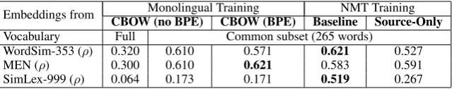
Embeddings from CBOW (no BPE) CBOW (BPE) Baseline Source-Only Vocabulary Full Common subset (265 words)
WordSim-353 (ρ) 0.320 0.610 0.571 0.621 0.527
MEN (ρ) 0.300 0.610 0.621 0.583 0.591
[image:3.595.141.461.62.125.2]SimLex-999 (ρ) 0.064 0.173 0.171 0.519 0.267
Table 2: Pairwise cosine distances between embeddings correlated with standard human judgments for the common subset of the vocabularies. Best result in each row in bold.
We used uniform distribution from 0 to 1 in the first experiment with embeddings and returned to the baseline normal distribution in subsequent ex-periments.
The best results we were able to obtain are from a third experiment “Larger Source-Only” with batch size increased to 150 but also with dif-ferences in other model parameters. (We ran this setup on a K80 card at Amazon EC2.) This run is therefore not comparable with any of the remain-ing runs, but we nevertheless submitted it as our secondary submission for the WMT 2017 training task (i.e. not to be evaluated manually).
2.3 Discussion
Due to lack of resources, we were not able to run pairs of directly comparable setups. As Fig-ure1however suggests, all our experiments with pre-trained embeddings performed well below the baseline of the 4GB model. This holds even for the larger model size.
2.3.1 Analysis of Embeddings
In search for understanding the failure of pre-trained embeddings,5we tried to analyze the em-beddings we are feeding and getting from our sys-tem.
Recent work by Hill et al. (2017) has demon-strated that embeddings created by monolingual models tend to model non-specific relatedness of words (e.g.teacherbeing related tostudent) while those created from NMT models are more ori-ented towards conceptual similarity (teacher ≈
professor) and lexical-syntactic information (the Mikolov-style arithmetic with embedding vectors for morphosyntactic relations like pluralization but not for “semantic” relations likeFrance-Paris). It is therefore conceivable, that embeddings pre-trained with the monolingual methods are not suit-able for NMT.
5This negative result actually contradicts another set of
experiments using the Google News dataset embeddings cur-rently carried out at our department.
We performed a series of tests to diagnose four sets of embeddings: the baseline for the compar-ison are embeddings trained monolingually with the CBOW model without BPE processing. BPE may have affected the quality of embeddings, so we also evaluate CBOW trained on the training corpus after applying BPE. These embeddings were used to initialize the Source-Only setup. Fi-nally two sets of embeddings are obtained from Neural Monkey after the NMT training: from the Baseline run (random initialization) and Source-Only (i.e. the CBOW model used in initialization and modified through NMT training).
The tests check the capability of the respective embeddings to predict similar words, as manually annotated in three different datasets: WordSim-353, MEN and Simlex-999. WordSim-353 and MEN contain a set of 353 and 3000 word pairs, respectively, rated by human subjects according to their relatedness (any relation between the two words). Simlex-999, on the other hand, is made up of 999 word pairs which were explicitly rated according to their similarity. Similarity is a spe-cial case of relatedness where the words are re-lated by synonymy, hyponymy, or hypernymy (i.e. an “is a” relation). For example,car is related to but not similar to road, however it is similar to automobile or to vehicle. Spearman’s rank cor-relation (ρ) is then computed between the ratings
of each word pair (v, w) from the given dataset
and the cosine distance of their word embeddings,
cos(emb(v),emb(w))over the entire set of word
pairs. The results of the tests are shown in Table2. The tests were performed for the intersecting subset of all four vocabularies, i.e. the words not broken by BPE and known to all three datasets. (265 words). For the CBOW embeddings which were trained without BPE being applied, the scores of the full vocabulary (which has a much higher coverage of the testing dataset pairs) is also included.
com-0 5 10
0 2 4 6 8 10 12 14 16 18 20
Decrease every 12h
Decrease every 24h
BLEU
Steps (in millions examples)
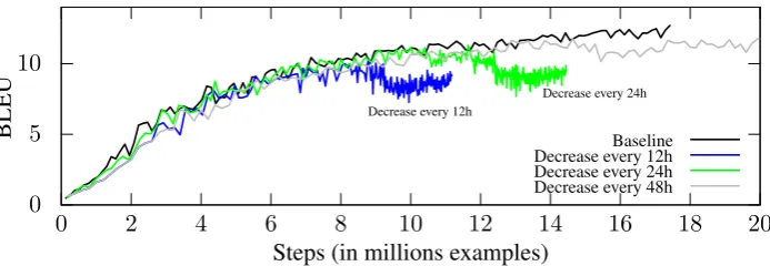
[image:4.595.126.473.70.190.2]Baseline Decrease every 12h Decrease every 24h Decrease every 48h
Figure 2: Results of mini-batch decrementation compared to baseline model.
Baseline Decrease every 12h Decrease every 24h Decrease every 48h*
Starting mini-batch Size 60 100 100 150
Lowest mini-batch Size 60 5 5 20
Decreased every — 12 hours 24 hours 48 hours
Table 3: The different setups with mini-batch size decrementation. The run reducing every 48h was our primary submission (*).
ing from NMT perform markedly better (0.519) than other embeddings. The embeddings extracted from the Source-Only model which was initialized with the CBOW embeddings score somewhere in the middle (0.267), which indicates that the NMT model is learning word similarity and it moves to-wards similarity from the general relatedness.
To a little extent, this is apparent even in the values of the embedding vectors of the individual words: we measured the cosine distance between the embedding attributed to a word by the Base-line NMT training and the embedding attributed to it by “CBOW (BPE)”. The average cosine dis-tance across all words in the common subset of vocabularies was 1.003. After the training from “CBOW (BPE)” to “Source-only”, the model has moved closer to the Baseline, having an average cosine distance of 0.995 (cosine of “Baseline” vs. “Source-only” averaged over all words in the com-mon subset). In other words, the training tried to “unlearn” something from the pre-trained CBOW (BPE).
For MEN, the general relatedness test set, CBOW (BPE) embeddings perform best (0.621) but Baseline NMT is also capable of learning these relations quite well (0.583). The Source-Only setup again moves somewhat to the middle in the performance.
The poor performance of the CBOW embed-dings on the full vocabulary (cf. columns 1 and 2 in Table2) can be attributed to a lack of sufficient coverage of less frequent words in the training
cor-pus. When “CBOW (no BPE)” is tested on the common subset of vocabulary, it performs much better. Our explanation is that words not broken by BPE are likely to be frequent words. If the corpus was not big enough to provide enough con-text for all the words which were tested against the human judgment datasets, suitable embeddings would only be learned for the more frequent ones (including those that were not broken by BPE). In-deed, 263 words out of the set of 265 are among the 10000 most frequent words in the full vocabu-lary (of size 350881).
3 Mini-Batch Sizing
The effect of mini-batch sizing is primarily com-putational. Theoretically speaking, mini-batch size should affect training time, benefiting from GPU parallelization, and not so much the final test performance. It is common practice to choose the largest mini-batch size possible, due to its com-putational efficiency. Balles, Romero, and Hen-nig (2016) have suggested that dynamic adapta-tion of mini-batch size can lead to faster conver-gence. What we experiment with in this set of ex-periments is a much naiver concept based on in-crementation and dein-crementation heuristics.
3.1 Decrementation
0 5 10
0 5 10 15 20 25 30 35 40 45 50 55
BLEU
Steps (in millions examples)
Increase every 12h Baseline
0 5 10 15
0 50 100 150 200 250 300
BLEU
Time (in hours)
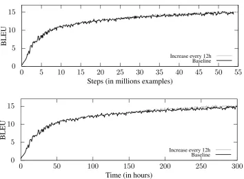
[image:5.595.122.477.66.326.2]Increase every 12h Baseline
Figure 3: Results of the setup with increasing mini-batch size.
approximation of the gradient of the entire train-ing set. Previous work byKeskar et al.(2016) has shown that models trained with smaller mini-batch size consistently converge to flat minima which re-sults in an improved ability to generalize (as op-posed to larger mini-batch size which tends to con-verge to sharp minima of the training function). By starting with a large mini-batch size, we aim to benefit from larger steps early in the training process (which means the optimization algorithm will proceed faster) and then to reduce the risk of over-fitting in a sharp minimum by gradually decrementing mini-batch size.
In the first experiment, our primary submission, we begin with the mini-batch size of 100 and de-crease it by 20 every 48 hours down to mini-batch size of 20. This was chosen heuristically.
In another two experiments, the mini-batch size was decremented every 12 hours and every 24 hours starting from 100 and reaching down to the size of 5. For these, the mini-batch size was re-duced by 20 at each interval till it reached 20, then it was halved twice and fixed at 5. A summary of the different mini-batch size decrementation set-tings tried can be seen in Table3.
The performance of the setups when reducing mini-batch is displayed in Figure 2. We see that the more often we reduce the size, the sooner the
model starts losing its performance.
The plots are the performance on a held-out dataset (as provided by the task organizers), so what we are be seeing is actually over-fitting, the opposite of what we wanted to achieve and what one would expect from better generalization.
3.2 Incrementation
Due to time and resource restrictions, we managed to complete the set of experiments with batch size increasing only after the deadline for the training task submissions. Interestingly, it is the only ex-periment which managed to outperform our base-line.
The model was trained for a week with batch size 65 and then for another week with mini-batch size increased to 100. Although both the baseline and this run are yet to converge, the in-creased mini-batch size resulted in a very small gain in terms of learning speed (measured in time), as seen in the lower part of Figure3. In terms of training steps, there is no observable difference.
4 Further Work 4.1 Mini-Batch Size
incre-mentation and decreincre-mentation functions or trying some method online mini-batch size adaptation, e.g. based on the dissimilarity of the current sec-tion of the corpus with the rest. This could be par-ticularly useful in the common technique of model fine-tuning when adapting to new domains.
Contrary to our expectations, reducing mini-batch size during training leads to a loss on both the heldout dataset and the training dataset. It is therefore not a simple overfitting but rather gen-uine loss in ability to learn. We assume that the larger mini-batch size plays an important role in model regularization and reducing it makes the model susceptible to keep falling into very local optima. Our not yet published experiments how-ever suggest that if we used the smaller mini-batch from the beginning, the model would not perform badly, which is worth further investigation.
4.2 Pre-Trained Embeddings
The word2vec embeddings were not suitable for the model. Scaling the whole embedding vector space so that the euclidean distances are very small but the cosine dissimilarities are preserved could make it easier for the translation model to adjust the embeddings but so far we did not manage to obtain any positive results in this respect.
We can also speculate that since NMT models produce embeddings which are best suited to the translation task, initializing word embeddings us-ing embeddus-ings from previously trained models could be a promising method of speeding up train-ing.
5 Conclusion
In our submission to the WMT17 Training Task, we tried two approaches: varying the mini-batch size on the fly and initializing the models with pre-trained word2vec embeddings. None of these techniques resulted in any improvement, except for a setup with mini-batch incrementation where at least the training speed in wallclock time in-creased (thanks to better use of GPU).
When analyzing the failure of the embeddings, we confirmed the observation byHill et al.(2017) than NMT learns direct word similarity while monolingual embeddings (CBOW) learn general word relatedness.
Acknowledgments
We would like to thank Jindˇrich Helcl and Jindˇrich Libovick´y for their advice and their previous work that we were able to use.
This work has been supported by the EU grant no. H2020-ICT-2014-1-645452 (QT21), as well as by the Ministry of Education, Youth and Sports of the Czech Republic SVV project no. 260 453.
Computational resources were in part supplied by the Ministry of Education, Youth and Sports of the Czech Republic under the Projects CES-NET (Project No. LM2015042), CERIT-Scientific Cloud (Project No. LM2015085) provided within the program Projects of Large Research, Develop-ment and Innovations Infrastructures. We are also grateful for Amazon EC2 vouchers we obtained at MT Marathon 2016.
References
Bahdanau, Dzmitry, Kyunghyun Cho, and Yoshua Ben-gio. (2014). Neural Machine Translation by Jointly Learning to Align and Translate. CoRR. arXiv: 1409.0473v7.
Balles, Lukas, Javier Romero, and Philipp Hennig. (2016). Coupling adaptive batch sizes with learning rates. Computing Research Repository. arXiv: 1508.07909v1.
Bojar, Ondˇrej, Jindˇrich Helcl, Tom Kocmi, Jindˇrich Li-bovick´y, and Tom´aˇs Musil. (2017). Results of the WMT17 Neural MT Training Task. InProceedings of the Second Conference on Machine Translation (WMT17), Copenhagen, Denmark.
Helcl, Jindˇrich and Jindˇrich Libovick´y. (2017). Neural Monkey: An open-source tool for sequence learn-ing. The Prague Bulletin of Mathematical Linguis-tics.doi:10.1515/pralin-2017-0001.
Hill, Felix, Kyunghyun Cho, S´ebastien Jean, and Yoshua Bengio. (2017). The representational geom-etry of word meanings acquired by neural machine translation models. Machine Translation. doi: 10.1007/s10590-017-9194-2.
Keskar, Nitish Shirish, Dheevatsa Mudigere, Jorge No-cedal, Mikhail Smelyanskiy, and Ping Tak Peter Tang. (2016). On large-batch training for deep learning: Generalization gap and sharp minima.
arXiv:1609.04836v2.
Mikolov, Tom´aˇs, Kai Chen, Greg Corrado, and Jeffrey Dean. (2013)a. Efficient Estimation of Word Rep-resentations in Vector Space. Computing Research Repository.arXiv:1301.3781v3.
Mikolov, Tom´aˇs, Ilya Sutskever, Kai Chen, and Greg Corrado. (2013)b. Distributed Representations of Words and Phrases and their Compositionality.
arXiv:1310.4546v1.
ˇReh˚uˇrek, Radim and Petr Sojka. (2010). Software Framework for Topic Modelling with Large Cor-pora. InProceedings of the LREC 2010 Workshop on New Challenges for NLP Frameworks, pages 45– 50, Valletta, Malta. ELRA.