Investigation into the Performance of a MIMO System Equipped with ULA or UCA Antennas: BER, Capacity and Channel Estimation

Investigation into the Performance of a MIMO System

Equipped with ULA or UCA Antennas: BER, Capacity

and Channel Estimation

Xia LIU1_{, Marek E. BIALKOWSKI}2_{, Feng WANG}1_{, Konstanty BIALKOWSKI}3

1_{Student Member IEEE, School of ITEE, The University of Queensland, Brisbane, Australia} 2_{Fellow IEEE, School of ITEE, The University of Queensland, Brisbane, Australia}

3_{Member IEEE, NationalICT Australia-Queensland Lab, Brisbane, Australia}

Email:{xialiu, meb, fwang, ksb}@itee.uq.edu.au

Received June 15, 2009; revised July 27, 2009; accepted August 30, 2009

ABSTRACT

This paper reports on investigations into the performance of a Multiple Input Multiple Output (MIMO) wireless communication system employing a uniform linear array (ULA) at the transmitter and either a uni-form linear array (ULA) or a uniuni-form circular array (UCA) antenna at the receiver. The transmitter is as-sumed to be surrounded by scattering objects while the receiver is postulated to be free from scattering ob-jects. The Laplacian distribution of angle of arrival (AOA) of a signal reaching the receiver is postulated. The performance of bit error rate (BER), capacity and channel estimation for a MIMO system are evaluated for the two cases that the receiver is equipped with ULA or with UCA antennas.

Keywords: MIMO, BER, BPSK, FSK, Channel Capacity, EDOF, Channel Estimation, ULA, UCA, Spatial Correlation

1. Introduction

In recent years, there has been a growing interest in the communication research community in the signal trans-mission technique employing multiple element antennas both at the transmitter and receiver sides of a wireless communication system. The reason is that it can sig-nificantly improve the transmission quality in terms of data throughput (capacity) and coverage area without the need for extra operational frequency bandwidth. Known as the multiple-input multiple-output (MIMO) technique, it is one of the promising techniques for the next genera-tion of mobile communicagenera-tions. For its physical imple-mentation, the MIMO technique frequently assumes uniform linear arrays (ULA) at both the transmitter and receiver ends of a wireless communication system. However, to obtain operation with larger angular views, uniform circular arrays (UCA) and their similarities such as triangular, square, pentagonal or hexagonal arrays are also considered. It can be expected that different con-figurations of antenna arrays will result in different spa-tial correlations of transmitted/received signals and thus they will influence channel properties between

transmit-ter and receiver in a different way. It is well known that MIMO channel capacity performance is based on the properties or channel matrix. According to [1] and [2], MIMO system BER performance and training-based channel estimation performance are determined by the channel correlation matrix which is affected by channel properties. These, in turn, the MIMO systems employ ULA or UCA receiver will affect the bit error rate (BER), channel estimation and the MIMO system capacity dis-tinctly.

2. System Model

2.1. System Configuration and Spatial Correlations

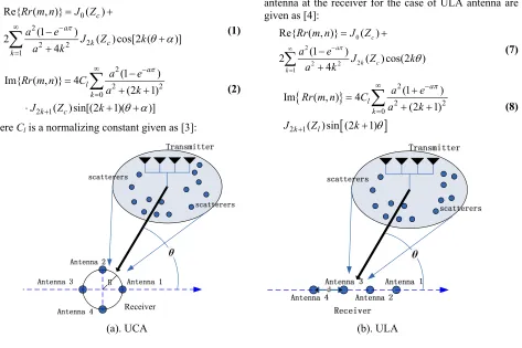
Figure 1 shows the configuration of the investigated MIMO system. The case of 4x4 MIMO is considered.

The transmitter is assumed to be equipped with a ULA antenna surrounded by scattering objects that are uni-formly distributed in a circle. Antenna elements in the array have an omnidirectional radiation pattern in the azimuth plane. The considered case represents a mobile station operating close to the ground where many sur-rounding obstacles are expected. In turn, the receiver is assumed to be equipped with either ULA or UCA of om-nidirectional antenna elements free from any surrounding obstacles. This configuration can represent a base station with antennas located high above the ground where there are no scattering objects.

In Figure 1, θ stands for the central AOA which is de-termined by the physical position of dominant scatterers with respect to the receiving antenna array. Assuming that the AOA follows the Laplacian distribution, the mathematical expressions for the real and imaginary parts of spatial correlation between the m-th and n-th antenna for the case of UCA receiving antenna are given as [3]:

0 2

2 2 2 1

Re{ ( , )} ( )

(1 )

2 ( ) cos[2

4

c a

k c k

Rr m n J Z

a e

J Z k

a k



( )]

 



 



 



2 2 0 2 1

(1 )

Im{ ( , )} 4

(2 1) ( )sin[(2 1)( )]

a l

k k c

a e

Rr m n C

a k

J Z k



 

 





 

 

 





(2)

where Cl is a normalizing constant given as [3]:

2(1 )

l a

a C

e



 (3)

with a representing a decay factor related to the angle spread (AS). When a increases the angle spread de-creases. J_n(.)is an n-th order Bessel function of the first kind. Zc is related to the antenna spacing and α is the

relative angle between the m-th and n-th antenna. If we let

1 2 R[cos( _m) cos( )]

K   _n



  (4)

2 2 R[sin( _m) sin( )]

K   _n



  (5)

where _mis the angle of m-th antenna in azimuthal planes, then:

2 2

2 2 2 2

1 sin( )

1 2

2 cos( )

1 2

1 2

c

K

K K

K

K K

Z K K













 

(6)

The mathematical expressions for real and imaginary components of spatial correlation between m-th and n-th antenna at the receiver for the case of ULA antenna are given as [4]:

0 2

2

2 2

1

Re{ ( , )} ( )

(1 )

2 ( ) c

4

c a

k c k

Rr m n J Z

a e

os(2 )

J Z k

a k





 



 

 











2 2 0 2 1

(1 )

Im ( , ) 4

(2 1)

( )sin (2 1)

a l

k k l

a e

Rr m n C

a k

J Z k





 





 

 





θ

Receiver

(a). UCA (b). ULA

0 0.5 1 1.5 2 2.5 3 0.2

0.4 0.6 0.8 1

d/λ

|R

(1,

2

)|,

S

C

b

et

w

ee

n 1 an

d 2 el

eme

nt

ULA SC pattern at central AOA = 60 deg

a = 3 a = 10 a = 30

0 0.5 1 1.5 2 2.5 3

0 0.2 0.4 0.6 0.8 1

d/λ

|R

(1,

2)

|, S

C

b

et

w

ee

n 1 and

2 el

eme

n

ULA SC pattern at central AOA = 30 deg

a = 3 a = 10 a = 30

0 0.5 1 1.5 2 2.5 3

0.5 0.6 0.7 0.8 0.9 1

d/λ

|R

(1

,2

)|,

S

C

be

tw

ee

n 1 an

d 2 el

eme

nt

ULA SC pattern at central AOA = 90 deg

a = 3 a = 10 a = 30

0 0.5 1 1.5 2 2.5 3

0 0.2 0.4 0.6 0.8 1

d/λ

|R

(1

,2

)|,

S

C

be

tw

e

en 1 a

nd 2 e

le

m

e

n

UCA SC pattern at central AOA = 30 deg

a = 3 a = 10 a = 30

0 0.5 1 1.5 2 2.5 3

0 0.2 0.4 0.6 0.8 1

d/λ

|R

(1,

2)

|, S

C

b

et

w

ee

n 1 and

2 el

eme

nt

UCA SC pattern at central AOA = 60 deg

a = 3 a = 10 a = 30

0 0.5 1 1.5 2 2.5 3

0 0.2 0.4 0.6 0.8 1

d/λ

|R

(1

,2

)|

, S

C

be

tw

ee

n 1 an

d 2 el

em

ent UCA SC pattern at central AOA = 90 deg

a = 3 a = 10 a = 30

Figure 2. Spatial correlation between antenna 1 and 2 for UCAandULA at AOA of 30o_{, 60}o _{and 90}o_.

where Zl = 2π(m-n)d/λ and d is antenna spacing.

The above expressions (1) (2) and (7) (8) can be ap-plied to determine spatial correlations between any two antenna elements in UCA or ULA receiving antennas. Note that these expressions do not include the effect of antenna mutual coupling. This condition is approximately fulfilled when the antenna element spacing is about half of the wavelength or more.

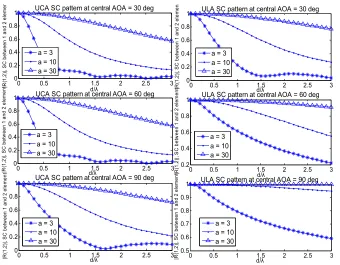
Figure 2 shows the spatial correlation between two antenna elements (1 and 2) of a UCA or ULA antenna when the central AOA is 30o_{, 60}o _{and 90}o_{. There are}

three curves in each plot. These curves correspond to a different decay factor a of 3, 10 and 30.

From the results presented in Figure 2, it is apparent that for the same antenna spacing d/λ the spatial correla-tion in ULA is higher than that in UCA when the central AOA increases from 30o to 90o_{. This can be due to the}

fact that ULA offers limited diversity when signals arrive from directions close to the ULA end-fire direction. UCA eliminates this deficiency as it offers almost a uni-form view angle for all directions.

2.2. Channel model

A flat block-fading narrow-band MIMO system with Mt

array antennas at transmitter and Mr array antennas at

receiver is considered. The relationship between the re-ceived and transmitted signals is given by (9):

( ) ( )

s

Y Hs t v t (9)

where Ys is the Mrx N complex matrix representing the

received signals; s(t) is the Mtx N complex matrix

rep-resenting transmitted signals at time domain t; H is the

Mrx Mt complex channel matrix and v(t) is the Mrx N

complex zero-mean white noise matrix at time domain t.

N is the length of transmitted signal. The channel matrix

H describes the channel properties which depend on an-tenna array configuration and signal propagation envi-ronment.

In order to simulate properties of the MIMO channel we apply the Kronecker model [5,6]. In this model, the transmitter and receiver correlations are assumed to be separable and the channel matrix H is represented as:

1/ 2 1/ 2

R g T

HR H R (10)

where Hg is a matrix with identical independent

dis-tributed (i.i.d) Gaussian entries with zero mean and unit variance and RR

}

and RT are spatial correlation matrices at

the receiver and transmitter, respectively. The channel correlation is expressed as,

{ H

H

R E HH (11)

where E{} stands for expected statistic value.

For the array configurations shown in Figure 1, the cor-relation experienced by pairs of transmitting antennas can be written as [7]:

0

( , ) [2 ( ) / ]

t

R m n J  m n  (12)

trans-t

M

r

M

 

mitting antennas can be generated using (13)

(1,1) (1, )

( ,1) ( , )

t t

t

t t t t t

R R

R

R M R M M

 

 

  

 

 



  



(13)

In turn, the correlation matrix for the receiving anten-nas, Rr, can be obtained using Equations (1) (2) and (7)

(8) and can be shown to be given as (14).

(1,1) (1, )

( ,1) ( , )

r r

r

r r r r r

R R

R

R M R M M

 

 

  



  



(14)

Having determined Rt and Rr, the channel matrix H

can be calculated using Equation (10).

3. BER Performance with BPSK Modulation

Scheme

3.1. BER Performance Analysis

Under a fading channel scenario, the average error prob-ability can be obtained by averaging the conditional error probability over the probability density function (pdf) of instantaneous SNR γ as:

0 ( | ) ( )

e

P 

_

To obtain p(γ), the method in [14] can be used to find the characteristic function Фγ of γ. By applying the

op-eration of an inverse Fourier transform (IFT) to the characteristic function, p(γ) can be derived. According to [1], the general expression for the characteristic function of γ is given as:

( ) | _r | m

M

w I nw R

m



 

   (16)

In which, w=t/ρ and ρ is the transmit SNR; m indicates the fading distribution properties. Such as m=1 and

m=1/2 corresponds Rayleigh and the one-sided Gaussian distribution, respectively; R is the channel correlation matrix.

Here, we assume the modulation schemes for the MIMO system under investigation are differential binary phase-shift key (DBPSK) and binary orthogonal fre-quency-shift key (BFSK). In the noncoherent case, the conditional BER for DBPSK and BFSK is given as [8],

1

( | ) exp( )

2

P e    (17)

in which α is modulation constant. BFSK corresponds to

α=1/2 and DBPSK corresponds to α=1. The average BER can be written as:

0

1

exp( ) ( )

2 1

( ) | 2 1

| |

2 r

noncoherent e

nt

m M

P P

t

I R

m

 

d

  









 

 

 



(18)

In turn, for the noncoherent case, the conditional BER for DBPSK and BFSK is given as [8],

( | ) ( 2 )

P e  Q  (19)

in which, Q(x) is Gaussian Q function and is expressed as [9],

2 /2

2 0

1

( ) exp( ) , 0

2sin

x

Q x  d x

 



_

The average BER can be written as

2 /2

2 0 0

/2

/sin 0

2

1

exp( ) ( )

2 sin

1

( ) |

1

| |

sin r coherent e

nt

m M

P d

t

I R d

m





  



P d

   



 _

 







 

 

 

 



3.2. Numerical Results

For the convenience of simulation, average BER of non-coherent DBPSK and BFSK are applied to evaluate the BER performance for the MIMO system. We assume that a ULA is present at the transmitter and either a UCA or ULA is located at the receiver. Simulations are per-formed for different values of the central AOA, decay factor, SNR and varying numbers of transmit/receive antennas.

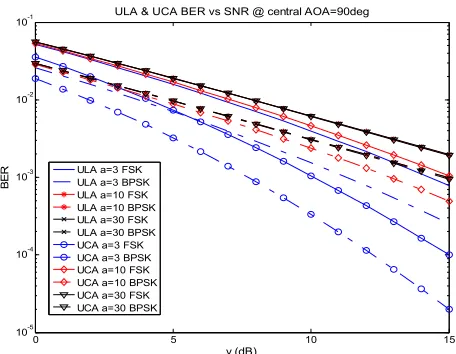
In the first scenario, 4-element array antennas are used at both the transmitter and receiver of a MIMO system. The spacing d between adjacent elements of ULA or the radius R of UCA at transmitter is set at 0.5 wavelength (λ). To reduce the antenna mutual coupling (which is neglected here) and correlation, d and R can be made larger than 0.5λ. Figures 3, 4, 5and 6 show BER as a function of SNR for both UCA and ULA for three values of decay factor a, and for the central AOA equal to 0o_,

30o_{, 60}o _{and 90}o_{. The modulation schemes are}

nonco-herent BFSK and DBPSK.

The presented results indicate that BER decreases when SNR increases. At a higher decay factor, BER performances are worse. This can be explained by the fact that a larger decay factor corresponds to a smaller angle spread (AS) indicating a higher spatial correlation level. BER performances are degraded due to correlation.

In Figures 3 and 4, one can see that for the central AOA of 0o _{and 30}o _{BER for both BFSK and DBPSK for ULA}

0 5 10 15

10-6

10-5

10-4

10-3

10-2

10-1 ULA & UCA BER vs SNR @ central AOA=0deg

γ (dB)

BER

ULA a=3 FSK ULA a=3 BPSK ULA a=10 FSK ULA a=10 BPSK ULA a=30 FSK ULA a=30 BPSK UCA a=3 FSK UCA a=3 BPSK UCA a=10 FSK UCA a=10 BPSK UCA a=30 FSK UCA a=30 BPSK

Figure 3. Noncoherent FSK and BPSK BER of UCA and ULA vs SNR at central AOA=0 o _{for three values of decay} factor a of 3, 10 and 30.

0 5 10 15

10-5

10-4

10-3

10-2

10-1 ULA & UCA BER vs SNR @ central AOA=60deg

γ (dB)

BE

R ULA a=3 FSK

ULA a=3 BPSK ULA a=10 FSK ULA a=10 BPSK ULA a=30 FSK ULA a=30 BPSK UCA a=3 FSK UCA a=3 BPSK UCA a=10 FSK UCA a=10 BPSK UCA a=30 FSK UCA a=30 BPSK

Figure 5. Noncoherent FSK and BPSK BER of UCA and ULA vs SNR at central AOA=60 o _{for three values of decay} factor a of 3, 10 and 30.

better than BFSK.

However, when the central AOA is increased to 60o

and 90o _{an opposite result is observed in Figures 5 and 6.}

In the latter case, performance of UCA is superior in comparison with ULA. These opposite trends indicate that at a certain value of central AOA, the performances of UCA and ULA should be equal.

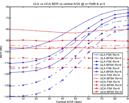
In order to determine the cross point (for BER) further simulations are performed. The results are shown in Fig-ure 7. BER is presented in unit of dB. One can see in Figure 7 that BER for ULA increases when the central AOA increases. This is because the ULA’s spatial corre-lation level increases as the central AOA gets larger. While the BER curve for UCA is almost constant through the central AOA range. The cross point is be-

0 5 10 15

10-6

10-5

10-4

10-3

10-2

10-1 ULA & UCA BER vs SNR @ central AOA=30deg

γ (dB)

BE

R ULA a=3 FSK

ULA a=3 BPSK ULA a=10 FSK ULA a=10 BPSK ULA a=30 FSK ULA a=30 BPSK UCA a=3 FSK UCA a=3 BPSK UCA a=10 FSK UCA a=10 BPSK UCA a=30 FSK UCA a=30 BPSK

Figure 4. Noncoherent FSK and BPSK BER of UCA and ULA vs SNR at central AOA=30 o _{for three values of decay} factor a of 3, 10 and 30.

0 5 10 15

10-5

10-4

10-3

10-2

10-1 ULA & UCA BER vs SNR @ central AOA=90deg

γ (dB)

BER

ULA a=3 FSK ULA a=3 BPSK ULA a=10 FSK ULA a=10 BPSK ULA a=30 FSK ULA a=30 BPSK UCA a=3 FSK UCA a=3 BPSK UCA a=10 FSK UCA a=10 BPSK UCA a=30 FSK UCA a=30 BPSK

Figure 6. Noncoherent FSK and BPSK BER of UCA and ULA vs SNR at central AOA=90 o _{for three values of decay} factor a of 3, 10 and 30.

tween approximate AOA=40o _{and AOA=50}o_{. To the left}

of the cross point, BER of ULA is lower than the one for UCA. In turn, on the right hand side, UCA’s perform-ance is better.

Using the earlier described settings for the 4x4 MIMO, the number of receiving antenna elements is increased and then the spatial correlation patterns and channel ca-pacity versus the number of transmit and receive anten-nas are simulated.

0 10 20 30 40 50 60 70 80 90 -120

-110 -100 -90 -80 -70

-60 ULA vs UCA BER vs central AOA @ γ=15dB & a=3

Central AOA (deg)

BE

R

(

dB

)

ULA FSK Rx=4 ULA BPSK Rx=4 UCA FSK Rx=4 UCA BPSK Rx=4

Figure 7. Noncoherent BFSK & DBPSK BER of UCA and ULA vs central AOA.

(a). ULA

(b). UCA

Figure 8. ULA and UCA antenna arrays.

Figure 8(a). In turn, for a UCA the number of antenna elements with the same spacing d increases on the circle, as shown in Figure 8(b). In the UCA case, when the number of elements on the circle increases with spacing d unchanged, the radius R increases correspondingly.

Figure 9 presents the spatial correlation between an-tenna elements 1 and 2 for receiving UCA and ULA for the new settings. From Figure 9(a), one can see that when the number of antenna elements increases the spa-tial correlation for UCA varies from 0 to 1. However, the variation due to an increased number of antenna ele-ments is very small. For the ULA case, the spatial corre-lation level of receiving antennas is unchanged when the number of antennas increases.

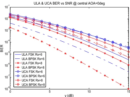
Similarly as Figures 3–6, Figures 10, 11 and 12 show the results of BER for a different number of receiving antenna elements for the cases of ULA and UCA receiveing

0 0.5 1 1.5 2 2.5 3

0 0.2 0.4 0.6 0.8 1

d/

|R

(2

,1

)|

B. ULA SC pattern with different number of Rx @ central AOA=30 and a=3

Number of Rx=4 Number of Rx=6 Number of Rx=8 Number of Rx=10

0 0.5 1 1.5 2 2.5 3

0 0.2 0.4 0.6 0.8 1

d/

|R

(2

,1

)|

A. UCA SC pattern with different number of Rx @ central AOA=30 and a=3 Number of Rx=4 Number of Rx=6 Number of Rx=8 Number of Rx=10

Figure 9. Spatial correlation between antenna 1 and an-tenna for different numbers (4,6,8,and 10) of anan-tenna ele-ments in receiving UCA (A) and ULA (B) antenna arrays at central AOA of 30° and decay factor a of 3.

0 5 10 15

10-8 10-7

10-6 10-5 10-4 10-3 10-2

10-1 ULA & UCA BER vs SNR @ central AOA=0deg

γ (dB)

BER

ULA FSK Rx=6 ULA BPSK Rx=6 ULA FSK Rx=8 ULA BPSK Rx=8 UCA FSK Rx=6 UCA BPSK Rx=6 UCA FSK Rx=8 UCA BPSK Rx=8

Figure 10. ULA vs UCA BER with different number of Rx antenna array elements at decay factor a equal to 3 and central AOA equal to 0o_.

antennas. An increase in the number of antenna elements in ULA and UCA brings improvement to the BER per-formance. The cross points between red curves repre-senting ULA and blue curves standing for UCA move to the right from approximate 40° to 50° as the number of antennas increases.

4. MIMO Channel Capacity with Perfect

Knowledge of Channel Matrix

4.1. MIMO Channel Capacity & EDOF

If CSI is perfectly known at the receiver but unknown at the transmitter, the capacity of a MIMO system with Mr

deter-mined using [10,11]:

2

(log {det[ _R ( H)]})

M t

C E I HH

M



  (22)

where {.}H _{stands for the transpose-conjugate; ρ is the}

total transmitted SNR.

An alternative expression for the capacity in such a case can be obtained by decomposing the channel into n = min(Mr, Mt) virtual single input single output (SISO)

sub-channels, and can be shown to be given as (23),

2

log (1 )

n

i i i

C

n

 _





where

n

i i





and the gains of sub-channels are represented by the ei-genvalues of the channel correlation matrix HHH_.

Here, it is assumed that the transmitted power is equally allocated to each sub-channel, which is easy to accomplish in practice. The channel capacity can be fur-ther maximized by applying power allocation schemes such as ‘water-filling’. However, this is not easy to im-plement, as CSI is required at the transmitter, which must be sent from the receiver to the transmitter.

It has to be noted that the MIMO channel capacity can be related to the channel effective degree of freedom (EDOF) [12]. In order to determine EDOF, the channel matrix properties and the signal to noise ratio (SNR) are required. According to [12], the EDOF is defined as:

0

(2 )

d

EDOF C

d 





 

 (24)

Given the eigenvalues of the channel correlation HHH_,

it can be rewritten as

2

0 0

2

(2 ) [log (1 )]

1

n n i

i

i i

i

d d _n

C

d d n

n 



 

  

 



    _

  







It is apparent that when ρλi /n >>1, (18) is approxi-mately equal to n and EDOF becomes maximum. In this case, every sub-channel is useful to transmit signals. In turn, when ρλi/n <1, EDOF is smaller than n, some sub-channels are not efficient to transmit signals. Rea sons for the reduced EDOF can be due to an increased level of channel correlation and decreased SNR.

4.2. Numerical Results

Based on the presented theory, the channel EDOF and capacity are simulated for a 4x4 MIMO system. The

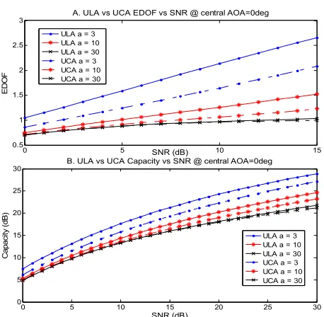
spacing d between adjacent elements of ULA or the ra-dius R of UCA at transmitter is set at 0.5 wavelength (λ). Figures 13, 14, 15and 16 show EDOF and capacity as a function of SNR for both UCA and ULA for three values of decay factor a, and for the central AOA equal to 0o_,

30o_{, 60}o _{and 90}o_.

The presented results reveal that both EDOF and ca-pacity increase when SNR increases. At a higher decay factor, both EDOF and capacity are lower. This is be-cause of the fact that a larger decay factor corresponds to a smaller angle spread (AS) indicating a higher spatial correlation level. EDOF and capacity are degraded due to correlation.

In Figures 13 and 14, one can see that for the central AOA of 0o _{and 30}o _{both EDOF and capacity for ULA are}

higher than for UCA for the three chosen values of decay factor.

0 5 10 15

10-7

10-6

10-5

10-4

10-3

10-2

10-1 ULA & UCA BER vs SNR @ central AOA=90deg

γ (dB)

BER

ULA FSK Rx=6 ULA BPSK Rx=6 ULA FSK Rx=8 ULA BPSK Rx=8 UCA FSK Rx=6 UCA BPSK Rx=6 UCA FSK Rx=8 UCA BPSK Rx=8

Figure 11. ULA vs UCA BER with different number of Rx antenna array elements at decay factor a equal to 3 and central AOA equal to 90o_.

0 10 20 30 40 50 60 70 80 90 -140

-130 -120 -110 -100 -90 -80 -70

-60 ULA vs UCA BER vs central AOA @ γ=15dB & a=3

Central AOA (deg)

BER (d

B

)

ULA FSK Rx=4 ULA BPSK Rx=4 ULA FSK Rx=6 ULA BPSK Rx=6 ULA FSK Rx=8 ULA BPSK Rx=8 UCA FSK Rx=4 UCA BPSK Rx=4 UCA FSK Rx=6 UCA BPSK Rx=6 UCA FSK Rx=8 UCA BPSK Rx=8

0 5 10 15 0.5

1 1.5 2 2.5

3 A. ULA vs UCA EDOF vs SNR @ central AOA=0deg

SNR (dB)

ED

O

F

ULA a = 3 ULA a = 10 ULA a = 30 UCA a = 3 UCA a = 10 UCA a = 30

0 5 10 15 20 25 30

0 5 10 15 20 25

30 B. ULA vs UCA Capacity vs SNR @ central AOA=0deg

SNR (dB)

Capa

ci

ty

(

dB

)

ULA a = 3 ULA a = 10 ULA a = 30 UCA a = 3 UCA a = 10 UCA a = 30

Figure 13. EDOF and capacity of UCA and ULA vs SNR at central AOA=0 o _{for three values of decay factor a of 3, 10} and 30.

0 5 10 15

0.8 1 1.2 1.4 1.6 1.8 2

2.2 A. ULA vs UCA EDOF vs SNR @ central AOA=60deg

SNR (dB)

ED

O

F

ULA a = 3 ULA a =10 ULA a = 30 UCA a = 3 UCA a = 10 UCA a = 30

0 5 10 15 20 25 30

0 5 10 15 20 25

30 B. ULA vs UCA Capacity vs SNR @ central AOA=60deg

SNR (dB)

Capac

ity

(

dB

)

ULA a = 3 ULA a = 10 ULA a = 30 UCA a = 3 UCA a = 10 UCA a = 30

Figure 15. EDOF and capacity of UCA and ULA vs SNR at central AOA=60o _{for three values of decay factor a of 3, 10} and 30.

When the central AOA is increased to 60o _{and 90}o _an

opposite result is observed in Figure 5 and 6. In the latter case, performance of UCA is superior in comparison with ULA.

To determine the cross point (for EDOF or capacity) further simulations are performed. The results are shown in Figure 17. One can see in Figure 17 that both EDOF and capacity decrease for the case of ULA when the cen-tral AOA increases at two different SNR. This is because the ULA’s spatial correlation level increases as the central

0 5 10 15 20 25 30

0 5 10 15 20 25

30 B. ULA vs UCA Capacity vs SNR @ central AOA=30deg

SNR (dB)

C

ap

ac

ity

(

dB

)

ULA a = 3 ULA a = 10 ULA a = 30 UCA a = 3 UCA a = 10 UCA a = 30

0 5 10 15

0.5 1 1.5 2

2.5 A. ULA vs UCA EDOF vs SNR @ central AOA=30deg

SNR (dB)

ED

O

F

ULA a = 3 ULA a = 10 ULA a = 30 UCA a = 3 UCA a = 10 UCA a = 30

Figure 14. EDOF and capacity of UCA and ULA vs SNR at central AOA=30 o _{for three values of decay factor a of 3, 10} and 30.

0 5 10 15

0.8 1 1.2 1.4 1.6 1.8 2

2.2 A. ULA vs UCA EDOF vs SNR @ central AOA=90deg

SNR (dB)

EDO

F

ULA a = 3 ULA a = 10 ULA a = 30 UCA a = 3 UCA a = 10 UCA a = 30

0 5 10 15 20 25 30

0 5 10 15 20 25

30 B. ULA vs UCA Capacity vs SNR @ central AOA=90deg

SNR (dB)

Capac

ity

(

dB

)

ULA a = 3 ULA a = 10 ULA a = 30 UCA a = 3 UCA a = 10 UCA a = 30

Figure 16. EDOF and capacity of UCA and ULA vs SNR at central AOA=90o_{for three values of decay factor a of 3, 10} and 30.

AOA gets larger. This degrades channel capacity. The cross point is between AOA=40o _{and AOA=50}o_{. To the}

left of the cross point, EDOF and capacity of ULA is higher than for UCA. In turn, on the right hand side, UCA’s performance is better.

The cross points between red curves representing ULA and blue curves standing for UCA move to the right as the number of antennas increases. When the number of receiving antenna elements is 10, the capacity of ULA is superior to UCA for the central AOA of 0o _{to 50}o_.

5. MIMO Channel Estimation

For the training based channel estimation method, the relationship between the received signals and the training sequences is given by Equation (26) as

Y HP V (26)

0 10 20 30 40 50 60 70 80 90 1

1.2 1.4 1.6 1.8 2 2.2 2.4 2.6

2.8 ULA vs UCA EDOF vs central AOA @ a = 3

Central AOA (deg)

EDO

F

ULA SNR = 10dB UCA SNR = 10dB ULA SNR = 15dB UCA SNR = 15dB

0 10 20 30 40 50 60 70 80 90 4

5 6 7 8 9 10 11

12 ULA vs UCA Capacity vs central AOA @ a=3

Central AOA (deg)

C

hanne

l C

apa

ci

ty

ULA SNR = 10dB UCA SNR = 10dB ULA SNR = 15dB UCA SNR = 15dB

Figure 17. EDOF and capacity of UCA and ULA vs central AOA.

0 5 10 15 20 25 30 5

10 15 20 25 30

35 ULA vs UCA Capacity with different number Rx antennas @ central AOA=0deg

SNR (dB)

Cap

ac

ity

(

dB

)

ULA Number of Rx=4 ULA Number of Rx=6 ULA Number of Rx=8 ULA Number of Rx=10 UCA Number of Rx=4 UCA Number of Rx=6 UCA Number of Rx=8 UCA Number of Rx=10

Figure 18. ULA vs UCA capacity with different number of Rx antenna array elements at decay factor a equal to 3 and central AOA equal to 0o_.

0 5 10 15 20 25 30

5 10 15 20 25 30

35 ULA vs UCA Capacity with different number Rx antennas @ central AOA=90deg

SNR (dB)

C

apa

ci

ty

(

dB

)

ULA Number of Rx=4 ULA Number of Rx=6 ULA Number of Rx=8 ULA Number of Rx=10 UCA Number of Rx=4 UCA Number of Rx=6 UCA Number of Rx=8 UCA Number of Rx=10

Figure 19. ULA (blue lines) vs UCA (red lines) capacity for different number of Rx antenna array elements at decay factor a equal to 3 and central AOA equal to 90o_.

0 10 20 30 40 50 60 70 80 90 16

17 18 19 20 21 22 23 24 25

26 ULA vs UCA Capacity vs central AOA with different number of Rx antennas at SNR=15dB

Central AOA (deg)

C

han

nel

C

apa

ci

ty

ULA Number of Rx=4 ULA Number of Rx=6 ULA Number of Rx=8 ULA Number of Rx=10 UCA Number of Rx=4 UCA Number of Rx=6 UCA Number of Rx=8 UCA Number of Rx=10

Figure 20. ULA vs UCA capacity with different number of Rx antenna array elements decay factor a equal to 3.

Here the transmitted signal S in (1) is replaced by P, which represents the Mt x L complex training matrix

(sequence) where L is the length of the training sequence. The goal is to estimate the complex channel matrix H

from the knowledge of Y and P. The transmitted power in the training mode is assumed to be given by a constant value. According to [13] and [14], the estimation using SLS or MMSE method requires orthogonality of the training matrix P. In the undertaken analysis, the training matrix P is assumed to satisfy this condition.

The performance of SLS method can be obtained by scaling up the results from the least square (LS) method. Using the LS method, the estimated channel can be writ-ten as [13,14],

†

ˆ LS

where {.}† _{stands for pseudo-inverse. The mean square}

error (MSE) of the LS method is given as 2

ˆ {

LS LS _F}

MSE E H H (28)

in which E{.} denotes a statistical expectation. Accord-ing to [13] and [14], the minimum value of MSE for the LS method is given as

2

min

LS t r

t M M MSE



 (29)

in which ρt _{stands for transmitted SNR in training}

mode.

The SLS method reduces the estimation error of the LS method and the improvement is given by the scal-ing factor γ as

{ } { }

H

LS H

tr R

MSE tr R

 

 (30)

The estimated channel matrix is represented by [13,14]

†

2 1

{ }

ˆ

{( ) } { }

H

SLS H

n r H

tr R

H YP

M tr PP tr R

 



  (31)

Here, σn2 _{is the noise power; R}

H is the channel

correla-tion matrix defined as RH=E{HHH} and tr{.} implies the

trace operation.

The MSE for SLS is given as [13,14]

2

2 2

ˆ

{ }

(1 ) { }

SLS LS _F

H LS

MSE E H H

tr R MSE



 

 

  

(32)

The minimized MSE of MMSE method can be written as [7,8]

min

{ } { }

SLS LS H

LS H

MSE tr R MSE

MSE tr R



 (33)

By taking into account expression (23), the mini-mized MSE of the SLS method (27) can be rewritten as

1 1

2

1 1

2

[( { }) ]

[( ) ]

t

SLS H

t r

n

t i

i t r

M SE tr R

M M

M M



 

 

 

 





(34)

where n=min(Mr, Mt) and is λi the i-th eigenvalue of

the channel correlation RH.

In the MMSE method, the estimated channel matrix is given as (35) [13,14],

2 1

ˆ ₍ H ₎ H

MMSE H n r H

H _Y P R P_ M I  P R ₍₃₅₎

The MSE of MMSE estimation is given as 2

ˆ

{ }

in which RE is estimation error correlation written as

1 2 1 1

ˆ ˆ

{( )( ) }

( )

H

E MMSE MMSE

H

H n r

R E H H H H

R M PP 

  

  (37)

The minimized MSE for MMSE is obtained as [7,8]

1 2 1 1

{( H H ) }

MMSE n r

MSE _tr _{ } M Q PP Q  ₍₃₈₎

In (38), Q is the unitary eigenvector matrix of RH and Λ is the diagonal matrix with eigenvalues of RH. The

minimized MSE for the MMSE method, given by Equa-tion (38), can be rewritten using the orthogonality prop-erties of the training sequence P and the unitary matrix Q, as shown by

1 1

1 1 1

{( ) }

( )

MMSE t r

n

i t r

i

MSE tr M I

M



 

 

  

  





1



(39)

From Equations (33), (38) and (39), one can see that MSE of SLS and MMSE methods depends on the chan-nel correlation which, in turn, is affected by the trans-mitter and receiver spatial correlations.

In the first instance, the SLS and MMSE channel es-timation methods are assessed via computer simulations. In the undertaken simulations, the transmitter of the MIMO system is assumed to be equipped with ULA while the receiver uses either UCA or ULA. The case of 4x4 MIMO system is considered. The simulations are performed for different values of central AOA, decay factor a and the transmitted SNR (ρt = ρ). The other as-sumptions are similar to the ones already described in Subsection 3.2.

Simulations of MSE as a function of ρ (ρ=Ps/σn2) for

the SLS and MMSE channel estimation are performed for two decay factors of 3 and 30 assuming the central AOA of 0o_{, 30}o_{, 60}o _{and 90}o_{. The results are shown in}

Figures 21, 22, 23and 24.

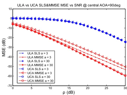
In all of the cases presented in Figures 21, 22, 23and 24 it is apparent that when ρ increases MSE decreases for both SLS and MMSE irrespectively from the choice of decay factor. MSE of SLS looks to be independent of the decay factor. Also only negligible changes in MSE of SLS are observed when CLA replaces ULA at the re-ceiver. However, MSE of MMSE is sensitive to the choice of decay factor and is smaller for larger decay factors.

With reference to the choice of the central AOA of 0o

and 30o _{in Figures 21 and 22, one can see that MSE of}

MMSE for ULA is larger than for UCA.

This happens irrespectively of the choice of the decay factor value. However, in the case of central AOA of 60o

and 90o_{, shown in Figures 23 and 24, one can see that the}

opposite conclusion takes place. The MSE of MMSE for the UCA is getting greater than when the ULA is used at the receiver.

{ }

MMSE MMSE _F E

0 5 10 15 20 25 30 -60

-50 -40 -30 -20 -10 0

10 ULA vs UCA SLS&MMSE MSE vs SNR @ central AOA=0deg

ρ (dB)

M

SE (

dB

)

ULA SLS a = 3 ULA MMSE a= 3 ULA SLS a = 30 ULA MMSE a = 30 UCA SLS a =3 UCA MMSE a=3 UCA SLS a = 30 UCA MMSE a = 30

Figure 21. MSE vs ρ for receiving ULA (blue lines) and UCA (red lines) at central AOA=0o_.

0 5 10 15 20 25 30

-60 -50 -40 -30 -20 -10 0

10 ULA vs UCA SLS&MMSE MSE vs SNR @ central AOA=30deg

ρ (dB)

M

SE (

dB)

ULA SLS a = 3 ULA MMSE a = 3 ULA SLS a = 30 ULA MMSE a = 30 UCA SLS a = 3 UCA MMSE a = 3 UCA SLS a = 30 UCA MMSE a = 30

Figure 22. MSE vs ρ for UCA and ULA at central AOA=30o_.

0 5 10 15 20 25 30

-60 -50 -40 -30 -20 -10 0

10 ULA vs UCA SLS&MMSE MSE vs SNR @ central AOA=60deg

ρ (dB)

M

SE (

dB)

ULA SLS a = 3 ULA MMSE a = 3 ULA SLS a = 30 ULA MMSE a = 30 UCA SLS a = 3 UCA MMSE a = 3 UCA SLS a = 30 UCA MMSE a = 30

Figure 23. MSE vs ρ for receiving ULA (blue lines) and UCA (red lines) at central AOA=60o_.

0 5 10 15 20 25 30

-70 -60 -50 -40 -30 -20 -10 0 10

ULA vs UCA SLS&MMSE MSE vs SNR @ central AOA=90deg

ρ (dB)

MS

E

(

dB

)

ULA SLS a = 3 ULA MMSE a = 3 ULA SLS a = 30 ULA MMSE a = 30 UCA SLS a = 3 UCA MMSE a = 3 UCA SLS a = 30 UCA MMSE a = 30

Figure 24. MSE vs ρ for receiving ULA (blue lines) and UCA (red lines) at central AOA=90o_.

0 10 20 30 40 50 60 70 80 90

-34 -32 -30 -28 -26 -24 -22 -20

-18 ULA vs UCA MSE vs central AOA

Central AOA (deg)

MS

E

(

dB

)

ULA MMSE ρ = 15dB

UCA MMSE ρ = 15dB

ULA MMSE ρ = 20dB

UCA MMSE ρ = 20dB

Figure 25. MSE vs central AOA for ULA (blue line) and UCA (red line) at decay factor a equal to 3.

Figure 25 shows the simulated results for MSE versus central AOA for two cases of ρ equal to 15dB and 20dB, respectively. One can see that when ρ is equal to 15dB, MSE of MMSE for ULA is larger than for UCA when the central AOA is smaller than 50o_{. In turn, when the}

central AOA is larger than 50o _{an opposite situation takes}

place: MSE of MMSE for UCA is larger than the one for ULA.

Similar observations are made when ρ is equal to 20dB. However, in this case the central AOA cross point is moved to about 60o_.

Figure 26 shows the results for MSE similar to those of Figure 25. However, they are obtained for different number of receiving antenna elements of 4, 6, 8 and 10.

It can be seen in Figure 26 that when the receiving ar-ray includes 4 antenna elements, the channel estimation shows the best performance for both ULA and UCA. When the number of antenna elements is increased from 4 to 6, 8 and 10, the channel estimation accuracy is get-ting worse for both ULA and UCA cases. These results confirm our expectation that larger size MIMO systems face the problem of decreased estimation of MIMO channel.

6. Conclusions

In this paper, we have reported on investigations into the performance of BER, channel capacity and channel es-timation of a MIMO system employing Uniform Linear Array at the transmitter and either a Uniform Circular Array or Uniform Linear Array at the receiver. In the presented investigations, the transmitter is assumed to be surrounded by scattering objects while the receiver is postulated to be free of scatterers. The signal angle of arrival (AOA) has been assumed to follow the Laplacian distribution. The angle spread (AS) is characterized by the decay factor.

The attention has been paid to the effect of different spatial correlation in receiving linear and circular arrays. The obtained results have shown that for the central AOA varying from 0o _{to 90}o_{, UCA’s spatial correlation}

pattern (as a function of element antenna spacing) is relatively constant while ULA’s spatial correlation level increases; both UCA’s and ULA’s spatial correlation patterns are not sensitive to the increased number of ar-ray elements.

At a larger decay factor corresponding to a smaller angular spread (and thus a higher level of spatial correla-tion), the BER of both FSK and BPSK are increased for both the UCA and ULA receiving antenna cases. Simu-lation results also presented the variation of BER as a function of central AOA varying from 0o _{to 90}o _{when the}

signal to noise ratio γ is equal to 15dB. It has been shown that at γ=15dB, BER for ULA is lower in comparison with UCA when the central AOA is smaller than 45o_.

When central AOA becomes larger than 50o_{, the UCA}

performance is better in terms of lower value of BER. When the number of receiving antennas increases, the performance gets better in terms of BER for both ULA and UCA cases.

The obtained results have also shown that for a larger decay factor, the channel capacity is reduced for both UCA and ULA receiving antennas. The 4x4 MIMO sys-tem employing the receiving ULA shows higher capacity when the central AOA is smaller than 40o_{. For central}

AOA greater than 50° the opposite happens and the sys-tem using UCA outperforms the one using ULA. When the number of receiving antennas increases, improve-ments to channel capacity are demonstrated for both ULA and UCA. The cross points for ULA and UCA ca-pacity curves move to the right when the number of an-tennas increases. When the number of receiving anan-tennas is 10, the capacity performance for ULA is superior to UCA for central AOA of 0o _{to 50}o_.

For channel estimation performance, at a larger decay factor, the MSE of training based channel estimation methods such as SLS and MMSE is reduced for both the UCA and ULA receiving antenna cases. This agrees with the findings of [15] and [16]. Other presented results have concerned the variation of MSE as a function of central AOA varying from 0o _{to 90}o _{when the signal to}

noise ratio ρ is equal to 15dB or 20dB. It has been shown that at ρ=15dB, MSE of MMSE for ULA is higher in comparison with UCA when the central AOA is smaller than 50o_{. When central AOA becomes larger than 50}o_,

the ULA performance is better in terms of lower value of MSE. For ρ of 20dB a similar trend has been observed but the cross point occurs for the central AOA equal to 60o_{. When the number of receiving antennas increases,}

the performance gets worse in terms of MSE for both ULA and UCA cases.

7. References

[1] J. Luo, J. R. Zeidler, and S. McLaughlin, “Performance analysis of compact antenna arrays with MRC in corre-lated Nakagami fading channels,” IEEE Transactions on Vehicular Technology, Vol. 50, No. 1, January 2001. [2] X. Liu, M. E. Bialkowski, and F. Wang, “Investigations

into the effect of spatial correlation on channel estimation and capacity of multiple input multiple output system,” International Journal of Communications, Network and System Sciences, Vol. 2, No. 3, June 2009.

[3] J. Tsai, R. M. Buehrer, and B. D. Woerner, “Spatial fad-ing correlation function of circular antenna arrays with Laplacian energy distribution,” IEEE Communications Letters, Vol. 6, No. 5, pp. 178–180, May 2002.

[5] E. G. Larsson and P. Stoica, “Space-time block coding for wireless communication,” Cambridge University Press, 2003.

[6] C. N. Chuah, D. N. C. Tse, and J. M. Kahn, “Capacity scaling in MIMO wireless systems under correlated fad-ing,” IEEE Transactions on Information Theory, Vol. 48, pp. 637–650, March 2002.

[7] W. C. Jakes, Microwave Mobile Communications, John Wiley & Sons, New York, 1974.

[8] J. G. Proakis, Digital Communications, 3rd Edition, McGraw-Hills, New York, 1995.

[9] M. Simon and M. S. Alouini, “A unified approach to the performance analysis of digital communication over gen-eralized fading channels,” Proceedings of IEEE, pp. 1860–1877, September 1998.

[10] E. Telatar, “Capacity of multi-antenna Gaussian chan-nels,” Europe Transactions on Telecommunication, Vol. 10, No. 6, pp. 585–596, November 1999.

[11] T. L. Marzetta and B. M. Hochwald, “Capacity of a mo-bile multiple-antenna communication link in Rayleigh flat fading,” IEEE Transactions on Information Theory, Vol. 45, No. 1, pp. 139–157, January 1999.

[12] D. Shiu, J. Foschini, M. J. Gans, and J. M. Kahn, “Fading correlation and its effect on the capacity of multielemnt antenna system,” IEEE Transactions on Communications, Vol. 48, No. 3, March 2000.

[13] M. Biguesh and A. B. Gershman, “MIMO channel esti-mation: Optimal training and tradeoffs between estima-tion techniques,” Proceedings of ICC’04, Paris, France, June 2004.

[14] M. Biguesh and A. B. Gershman, “Training-based MIMO channel estimation: A study of estimator tradeoffs and optimal training signals,” IEEE Transactions on Signal Processing, Vol. 54, No. 3, March 2006.

[15] X. Liu, M. E. Bialkowski, and S. Lu, “Investigations into training-based MIMO channel estimation for spatial cor-related channels,” Proceedings of IEEE AP-S Symposium, Hawaii, USA, 2007.