Estimating the effective population size from temporal allele frequency changes in experimental evolution

| INVESTIGATION

Estimating the Effective Population Size from

Temporal Allele Frequency Changes in

Experimental Evolution

Ágnes Jónás,*,†_{Thomas Taus,*},†_{Carolin Kosiol,}†_{Christian Schlötterer,}†_{and Andreas Futschik}†,‡,1

*Vienna Graduate School of Population Genetics, 1210 Vienna, Austria,†_{Institut für Populationsgenetik, Vetmeduni Vienna, 1210}

Vienna, Austria, and‡Department of Applied Statistics, Johannes Kepler Universität Linz, 4040 Linz, Austria ORCID ID: 0000-0002-7980-0304 (A.F.)

ABSTRACT The effective population size (Ne) is a major factor determining allele frequency changes in natural and experimental populations. Temporal methods provide a powerful and simple approach to estimate short-termNe:They use allele frequency shifts between temporal samples to calculate the standardized variance, which is directly related toNe:Here we focus on experimental evolution studies that often rely on repeated sequencing of samples in pools (Pool-seq). Pool-seq is cost-effective and often outper-forms individual-based sequencing in estimating allele frequencies, but it is associated with atypical sampling properties: Additional to sampling individuals, sequencing DNA in pools leads to a second round of sampling, which increases the variance of allele frequency estimates. We propose a new estimator ofNe;which relies on allele frequency changes in temporal data and corrects for the variance in both sampling steps. In simulations, we obtain accurateNeestimates, as long as the drift variance is not too small compared to the sampling and sequencing variance. In addition to genome-wideNeestimates, we extend our method using a recursive partitioning approach to estimateNelocally along the chromosome. Since the type I error is controlled, our method permits the identification of genomic regions that differ significantly in theirNeestimates. We present an application to Pool-seq data from experimental evolution withDrosophilaand provide recommendations for whole-genome data. The estimator is computationally efficient and available as an R package athttps://github.com/ThomasTaus/Nest.

KEYWORDSeffective population size; genetic drift; Pool-seq; experimental evolution

D

et al.2012; Longet al.2015; Schlöttereret al.2015). In sexually reproducing organisms, the census population size is typically keptfixed at fairly low numbers, rarely exceeding 2000 individ-uals. With such small population sizes, genetic drift causes sto-chasticfluctuations in allele frequencies. Under neutrality, the level of random frequency changes is determined by the

effec-tive population size (Ne) (Wright 1931). Furthermore, the effi -cacy of selection is influenced byNe:For weakly selected alleles, the probability offixation is directly proportional to the product ofNeand the intensity of selection (Fisher 1930; Kimura 1964). As changes in allele frequency are greatly affected by the pop-ulation size, it is fundamental to estimateNeaccurately to un-derstand molecular variation in experimental evolution studies. Krimbas and Tsakas (1971) estimated Ne using the stan-dardized variance of allele frequency (F, see also Falconer and Mackay 1996) from longitudinal samples in natural popula-tions of olive flies. AsFwas calculated from these samples, they accounted for the sampling variance that also contributed to the true allele frequency variance. This approach was fur-ther improved and used by several authors (Nei and Tajima 1981; Pollak 1983; Waples 1989; Jorde and Ryman 2007).

With the widespread availability of powerful computers, also maximum-likelihood-based methods became popular (Williamson and Slatkin 1999; Andersonet al.2000; Wang 2001; Hui and Burt 2015) in addition to the moment-based

Copyright © 2016 Jónáset al. doi: 10.1534/genetics.116.191197

Manuscript received May 4, 2016; accepted for publication July 30, 2016; published Early Online August 19, 2016.

Available freely online through the author-supported open access option.

This is an open-access article distributed under the terms of the Creative Commons Attribution 4.0 International License (http://creativecommons.org/licenses/by/4.0/), which permits unrestricted use, distribution, and reproduction in any medium, provided the original work is properly cited.

Supplemental material is available online atwww.genetics.org/lookup/suppl/doi:10. 1534/genetics.116.191197/-/DC1.

1_{Corresponding author: Department of Applied Statistics, Johannes Kepler Universität}

approaches discussed above. Although these methods show less bias than the moment-based approaches (Wang 2001), they are still computationally demanding, in particular for the large numbers of markers typically obtained with novel sequencing technologies (Follet al.2015).

EstimatingNewith temporal methods requires samples col-lected at least at two time points. Alternative methods that use only a single time point are based on linkage disequilibrium (LD) (Hill 1981; Waples and Do 2008, 2010; Waples and England 2011), heterozygote excess (Pudovkinet al.1996), molecular coancestry (Nomura 2008), sibship frequencies (Wang 2009, 2013), or combinations of summary statistics using approxi-mate Bayesian computation (Tallmon et al. 2008). LD-based methods are widespread but require haplotype or unphased diploid genotype information, which limits their applicability.

Although the cost for sequencing has dropped considerably, the separate sequencing of thousands of individuals in replicate populations in experimental evolution studies is still out of reach. Sequencing samples in pools (Pool-seq) can provide a cost-effective alternative (Schlöttereret al.2014). Pool-seq has also been shown to outperform individual-based sequencing in estimating allele frequencies and inferring population genetic parameters under several conditions (Futschik and Schlötterer 2010; Zhuet al.2012; Gautieret al.2013). For these reasons, Pool-seq has become the basis of many experimental evolution

“evolve and resequence”(E&R) studies (Turner et al.2011; Schlötterer et al. 2015). Following the emergence of E&R, many population genetic estimators have been adjusted to handle the properties of Pool-seq data (Futschik and Schlöt-terer 2010; Kofleret al. 2011a,b; Kolaczkowski et al.2011; Boitard et al.2013; Ferrettiet al.2013). To the best of our knowledge, noNeestimators have been developed so far that properly deal with Pool-seq data.

In this article, we present a novel temporal method to estimateNe from pooled samples. We show that previously proposed estimators can lead to substantial bias, as they ne-glect the variance component due to pooled sequencing. We introduce a new model accounting for the two-step sampling process associated with Pool-seq data. In thefirst sampling step individuals are drawn from the population to create pooled DNA samples. In the second step, pooled sequencing is modeled as binomial sampling of reads out of the DNA pool. We show on simulated data that our method outper-forms standard temporalNeestimators. For real data, we also suggest to use a segmentation algorithm, to partition the genome-wide sequence data into stretches of DNA with sig-nificantly differentNeestimates. Finally, we present an appli-cation to a genome-wide experimental evolution data set fromDrosophila melanogaster(Franssenet al.2015).

Materials and Methods

Sampling schemes

Nei and Tajima (1981) investigated the sampling properties of temporalNeestimators and proposed two different

sam-pling schemes. Under thefirst scheme (plan I), individuals are either sampled after reproduction or returned to the pop-ulation after their genotypes have been examined. In con-trast, under the second scheme (plan II) sampling takes place before reproduction and the sampled individuals are permanently removed from the population and their geno-types do not contribute to the next generation. By assuming different sampling distributions, they derived separate Ne estimators under sampling plans I and II.

Waples (1989) unified the calculations under the two plans by assuming binomial sampling out of an infinitely large paren-tal gamete pool for both sampling schemes. He concluded that the measure of variance under the two sampling plans differs only in a covariance term. For plan I, there is a positive corre-lation between allele frequencies sampledtgenerations apart because they are both derived from the same population at generation 0. In contrast, for plan II, the initial sample and individuals contributing to the next generation can be consid-ered as independent binomial samples; thus sample frequen-cies at generations 0 andtare uncorrelated.

For a typical E&R study, outbred experimental populations are created by mixing a large number of inbred lines (e.g., Turner and Miller 2012; Huang et al.2014; Franssenet al.

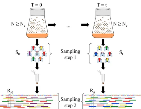
2015). The populations are then propagated under the de-sired experimental conditions while keeping the census size of the population controlled through time (Figure 1). How-ever, the experimenter has no direct influence on the effective population size, which is in general lower than the census size. In E&R studies with Drosophila, the census size rarely exceeds some hundreds of individuals, and sampling usually takes place after reproduction according to plan I. For organ-isms maintained at larger sizes, such as yeast, the sample for genetic analysis is not returned to the population (Burkeet al.

2014). Plan II applies to such cases.

In E&R studies, sampled individuals are often pooled to-gether for DNA extraction (Schlöttereret al.2014). The size of the pool can be as large as the whole population. Depend-ing on the experimental design, it is also possible that only a fraction of the population is sequenced, for instance, only females (Tobler et al. 2014; Franssenet al. 2015). Pooled individuals are used to create DNA libraries, which are, in turn, subjected to high-throughput sequencing.

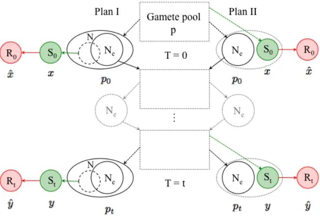
We consider two separate sampling steps when estimating

Ne from Pool-seq samples (Figure 1). In the first step, we model the sampling of individuals out of the population. This can take place according to either plan I or plan II. In the second step, we model the sequencing of a DNA pool by drawing reads at random with replacement from the fi rst-step sample. The allele frequency variance inferred from the sample is corrected for the additional variance coming from the two-step sampling and used for estimatingNe:

Notation

tgenerations apart to estimateNe(Figure 1) and denote the estimated effective population size by Nbe:Multiallelic sites in populations with low mutation rates, such asDrosophila, exist but are rare and likely to be sequencing errors (Burke et al.

2010). Therefore we consider only biallelic SNPs atn polymor-phic sites. At each sitei(i¼1. . .n) the true population allele frequency is denoted bypij at timeT¼j;wherej2 f0;tg:To

obtain allele frequency estimates for an unknownpij;the

pop-ulation is subjected to sampling. We consider two sampling steps (Figure 1). AtT¼j;wefirst sampleSjindividuals out of

the population to create a pooled DNA library for sequencing. Note that the number of sampled individuals is constant over thensites, and therefore the indexiis omitted here. Sampling individuals can take place according to either plan I or plan II, as described above (also shown in Supplemental Material,Figure S1). As the second sampling step, we model Pool-seq by draw-ing Rij reads out of the pooled DNA sample at each site i

(i¼1. . .n). This allows for variation in sequence coverage. Below we derive the variance in allele frequency for a given site. To keep notation simple, we omit again the indexiand denote the unknown sample allele frequency among theS0individuals at thefirst sampling time point (T¼0) byxand the subsequent allele frequency estimate obtained via pool sequencing fromR0 reads by^x:Similarly, at someT¼t;the respective frequencies are denoted byyand^y:Note that under pool sequencing only^x

and^yare observed.

Estimating Nefrom temporal allele frequency changes

Under neutral Wright–Fisher evolution the variance in allele frequency (s2

p) generated by drift aftertgenerations at a single

locus in a diploid population is well described by the expression

s2

p¼pð12pÞ

"

12 12 1

2Ne

!t#

; (1)

wherepis the starting allele frequency (Falconer and Mackay 1996). Wright (1931) denoted the standardized variance by

F¼s2

p=pð12pÞ; which leads to a convenient closed-form

expression for Ne: Furthermore, if Ne is large enough,

F12e2t=2Ne _andN

ecan be calculated as

Ne 2

t

2 lnð12FÞ: (2)

The relation between Ne and allele frequency changes de-scribed in Equation 1 wasfirst used by Krimbas and Tsakas (1971) in natural populations of oliveflies. They estimated the variance using

F¼Fa:¼1

a Xa

k¼1

ðxk2ykÞ2

xkð12xkÞ ;

(3)

where xk and yk (k¼1;. . .;a) are the observed allele

fre-quencies in the samples collectedtgenerations apart anda

is the number of alleles at a specific locus. To eliminate the contribution of sampling errors to the variance, the total var-iance Fa was corrected for the random sampling noise by

simply subtracting the corresponding variance. This ap-proach was further investigated and developed by a number of authors (Pamilo and Varvio-Aho 1980; Nei and Tajima 1981; Pollak 1983; Waples 1989).

Possible sources of bias inNeestimators were later inves-tigated by Jorde and Ryman (2007). The authors pointed out that the expectation overFis typically approximated by tak-ing the expected values separately for the numerator and the denominator (Turneret al.2001). They suggested a different weighting scheme of alleles leading to an alternative less-biased estimator to measure temporal frequency change.

Correction for two-step sampling

We consider a random-mating population with discrete gen-erations. Neutral evolution is assumed with no selection, migration, and mutation. Samples are drawn from the pop-ulation at generationsT¼0 andt. Throughout the derivation we consider diploid populations, and therefore a sample ofSj

individuals leads to 2Sj sequences at times T¼j2 f0;tg:

Sampling is assumed to be binomial with parameters 2Sj

andpj(Waples 1989). In the second sampling step at time T¼j;sequencing a random poolRjof reads is also modeled

as binomial sampling.

In analogy to Jorde and Ryman (2007), we use the follow-ing expression as our measure of the temporal change in allele frequency for biallelic sites,

Figure 1 Two-step sampling in experimental evolution withDrosophila. In E&R studies, populations are propagated at a census sizeNdefined by the experimenter, which is in general larger than the effective population size

Ne:Using temporal methods,Necan be estimated from the variance in allele frequency between samples takentgenerations apart. To get an accurate representation of allele frequencies in population genetic studies, a large number of individualsSj(j2 f0;tg) are sampled and pooled. Sampling can

take place according to sampling plan I or II based on the mode of repro-duction. Pooled samples are then subjected to high-throughput sequencing. Sequenced reads are subsequently aligned to the reference genome (shown at the bottom). We represent pool sequencing by an additional sampling step (called sampling step 2). We correct for both sampling steps when estimatingNein pooled samples. Additionally, we take into account variable coverage levels across the genome (coverageRijfor siteiatT¼j;j2 f0;tg)

Fc¼

ð^x2^yÞ2 ^

z2^x^y ; (4)

where^z¼ ð^xþ^yÞ=2:

The expectation ofFcfor a single biallelic locus is approx-imated by

EðFcÞ

Eð^x2^yÞ2 Eð^z2^x^yÞ¼

Varð^xÞ þVarð^yÞ22Covð^x;^yÞ Eðbz2bxbyÞ : (5)

For both plans, we derive expressions for the numerator and denominator in Equation 5 separately under the two-step sam-pling procedure, described above. Here we summarize our main conclusions; details on the derivation are provided inFile S1. WithCj:¼1=2Sjþ1=Rj21=2SjRjforj2 f0;tg;andp

denot-ing the true population allele frequency in the gamete pool at generation 0, we obtain

Varð^xÞ ¼pð12pÞC0; (6)

and

Varð^yÞ ¼pð12pÞ "

12ð12CtÞ 12 1 2Ne

!t#

: (7)

Note that Equations 6 and 7 differ only in the correction term

Cjfrom that in Waples (1989).

Waples (1989) previously showed that the denominator in Equation 5 reduces to

Eð^z2^x^yÞ ¼pð12pÞ2Covð^x;^yÞ: (8)

For plan II, Covð^x;^yÞ ¼0 (Waples 1989), andFccorrected for the noise coming from the two-step sampling for a single locus is given by

Fc9¼

Fc2C02Ct

12Ct : (9)

For plan I, on the other hand, the sample allele frequency at generation 0 is positively correlated to the sample allele frequency attbecause both are derived from the same pop-ulation at generation 0. This requires us to calculate the sample covariance Covð^x;^yÞ in Equation 5. It turns out (see File S1 for details) that the covariance of^x and ^yis equal to

Covð^x;^yÞ ¼pð12pÞ

2N ; (10)

whereNis the census size of the population at generation 0. Equation 10 is in agreement with the corresponding term of the standard methods (Waples 1989). Substituting the in-ferred covariance into Equation 5 leads to the following cor-rected variance estimate,Fc9for plan I

Fc9¼Fcð121=2NÞ2C02Ctþ1=N

12Ct  :

(11)

We provide the corresponding formulas ofFc9in haploid pop-ulations inFile S1.

With Pool-seq data, randomness in sequencing and local structures in the genome can lead to different coverage across marker sites, which we denote byRijfor sitei(i¼1;. . .n) and

timej(j2 f0;tg). In the genome-wide data set, we calculate

Fc9acrossnSNPs by summing over all loci in the numerator and denominator separately before carrying out the division in Equation 9, leading to the following weighting scheme for plan II:

Fc9¼

Pn

i¼1ð^xi2^yiÞ 2_2ð^

z_i2^x_i^y_iÞðCi0þCitÞ

Pn

i¼1ð^zi2^xi^yiÞð12CitÞ

: (12)

Similarly,Fc9can be calculated for plan I using Equations 4 and 11. Analogous to the single-locus case, our proposed estima-torsNbeðPÞfor a diploid population are obtained by plugging

Fc9into Equation 2.

Long time series have recently become available for some E&R experiments (Barrick et al. 2009; Burke et al. 2010, 2014). Standard Neestimators (Krimbas and Tsakas 1971; Nei and Tajima 1981; Waples 1989) assume a small number of generationsðtÞ and approximateNeusing 2Net=F:If, however,t=Neis larger, using this approximation can lead to severe bias (Figure S2). To avoid such a bias, we use Equation 2 to estimateNe:

Simulations

We evaluate the performance of our estimator on data sim-ulated under the neutral Wright–Fisher model. With a given population size of 2Ne;we simulate the frequency trajectory of nindependent SNPs. As we focus on biallelic SNPs, we assume two possible nucleotides (alleles) to be present in the population with given frequencies at the start. To create a new generation, nucleotides are drawn independently at random with a probability given by their respective allele frequencies in the old generation. The population is propa-gated at a constant size of 2Nefortnonoverlapping genera-tions. The effective population size is then estimated from allele frequencies inferred from Pool-seq samples taken from the population at the start and aftertgenerations. The sam-pling of individuals to create the pooled DNA library is sim-ulated by using sampling without replacement. To model the uneven coverage of genome-wide sequence data, we simu-late a random coverage for each site, using a Poisson distri-bution with parameter equal to the given mean coverage. For every position, reads are then generated by binomial sam-pling from the library with sample size equal to the local coverage.

while keeping the allele frequencies unchanged to avoid in-troducing additional sampling variance. We simulated each scenario 100 times.

Linkage disequilibrium between loci can reduce the num-ber of independent SNPs, thereby increasing the variance of the estimate. The impact of dependence between SNPs is investigated based on 10 replicated whole-genome forward simulations with recombination, using the software tool MimicrEE (Kofler and Schlötterer 2014). As a starting pop-ulation for the forward simpop-ulations, we sampled 2000 haploid genomes out of 8000 genomes simulated with fastsimcoal v.1.1.2 (Excoffier and Foll 2011; Bastide et al. 2013). The parameters used to generate the genomes mimic a wild pop-ulation ofD. melanogasterfrom Vienna (Fiston-Lavieret al.

2010; Bastide et al. 2013; Kofler and Schlötterer 2014). Allele counts are subjected to binomial sampling to mimic Pool-seq with a given sequence coverage.Neis estimated in nonoverlapping windows, each containing afixed number of SNPs.

Estimating Neon simulated data

We denote our estimator corrected for the additional sampling step,i.e., pooling, byNeðPÞ:We compareNeðPÞto the stan-dard estimators NeðWÞ and NeðJRÞ proposed by Waples (1989) and Jorde and Ryman (2007) that correct only for a single sampling step.

We illustrate experimental sampling procedures by con-sidering two major scenarios: (i) The full population is se-quenced as one large pool and (ii) only a subset of the population is used to create pooled samples. Under scenario (i) we simulate only a single binomial sampling step to represent sampling reads out of the DNA pool. The pool size is set to be equal to the census size of the population (Sj¼N),

and the number of sampled reads (Rij) represents the per-site

coverage. For estimators that correct only for a single sam-pling step, we use the coverage (Rij) as the sample size. For

scenario (ii), the sampled individuals (Sj) and the read

num-ber (Rij) represent the pool size and coverage forNeðPÞ:The coverage (Rij) is taken as the sample size for theNeðWÞand

NeðJRÞestimators, as these methods consider only one sam-pling step.

Change point inference for genome-wide estimates

The effect of genetic drift on the variance in allele frequency specified in Equation 1 holds only under the assumptions of Wright–Fisher neutral evolution. Deviations from the Wright– Fisher model, such as the presence of selection or demogra-phy, may cause systematically different changes in allele frequency, affecting the variance and causing locally vari-able patterns in genetic diversity. Furthermore, the effect of selection on one site of the genome may cause changes in the behavior of variants at nearby sites (Maynard Smith and Haigh 1974; Barton 2000; Comeronet al.2008). As a result, the estimates ofNeat different locations of the genome may deviate from the true number of breeding individuals in the population (Kimura and Crow 1963; Charlesworth 2009). For example, regions under background selection are as-sociated with reducedNbevalues that extend to linked sites due to the Hill–Robertson effect (Charlesworth 1996, 2012a; Comeronet al.2008). Similarly, selectively favorable alleles can also drag nearby neutral sites to high frequency (Maynard Smith and Haigh 1974), causing a local reduction in the esti-matedNe(Liu and Mittler 2008). Such an event is also known as a selective sweep (Berryet al.1991). On the other hand, we expect the opposite pattern,i.e., a local elevation ofNbefor types of selection such as balancing selection that maintain variation in the genome (Baysal et al.2007; Charlesworth 2009).

To detect such patterns inNbe;we apply a segmentation algorithm to partition the genome into locally homogeneous

b

Nestretches. We use a method related to an approach sug-gested by Futschiket al.(2014) for partitioning DNA sequences with respect to GC content. It is based on a statistical multiscale criterion and provides statistical error control, in the sense

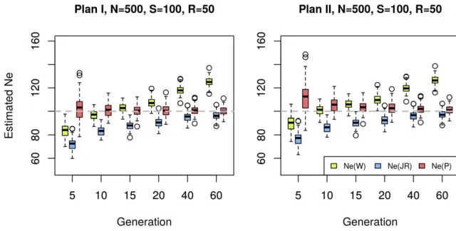
Figure 2 Effective population size estimated with different methods. Sixty generations of Wright– Fisher neutral evolution withNe¼100 diploid indi-viduals were simulated forn= 2000 unlinked loci (SNPs). Prior to sampling, the population was in-creased to a census size ofN¼500 individuals at each generation. At the starting population and at each indicated time point a sample was taken to create a pool ofS¼100 individuals. The pool was sequenced to an average coverage ofR¼50 and

Newas estimated on the resulting data set by sep-arately contrasting allele frequencies at generation 0 to each of the evolved generations denoted on thex-axis, usingNeðPÞ;NeðWÞ(Waples 1989), and

that the estimated number of windows will not exceed the true one except for a small error probabilityato be specified by the user. With ourNeestimates, we use a criterion pro-posed by Frick et al. (2014) for normally distributed re-sponses. It is implemented as part of the R package stepR

(Fricket al.2014). By using simulations with selection we also illustrate that this method is able to capture the signal of locally variableNbealong the chromosome.

Data availability

We estimatedNein an E&R study withD. melaongaster, pub-lished in Orozco-terWengelet al.(2012) and Franssenet al.

(2015). Pool-seq read libraries from these studies are available at the European Sequence Read Archive athttp://www.ebi.ac. uk/ena/under accession nos. ERP001290 and ERS460611– ERS460613.

Results and Discussion

Two-step correction is vital to avoid large bias inNbe

with Pool-seq data

Methods that do not correct for the additional sampling step caused by pooling can lead to substantial bias inNbeas illus-trated in Figure 2. Using simulated data, we compare our proposed estimatorNeðPÞto two commonly used estimators

NeðWÞ(Waples 1989) andNeðJRÞ(Jorde and Ryman 2007) that provide highly accurate estimates when only a single sampling event is simulated (Figure S3). Figure 2 shows that

the additional correction substantially decreases the bias for almost all scenarios (see alsoFigure S4,Figure S5, andFigure S6). Under plan I,NeðPÞis nearly unbiased. The plan II ver-sion of the estimator has a slight upward bias when applied on data simulated under plan I, if the samples are taken at very close time points.

As an alternative approach, we also estimated Ne sepa-rately for each locus, usingFc9in Equations 9 and 11. We then calculated the effective population size across thenloci as the harmonic mean over the single-locus Nbe estimates (Nb

* eðPÞ) (Peel et al. 2013). In our simulations, the harmonic mean estimator shows an accuracy similar to that of the original

b

NeðPÞ(Figure S7). However, fortlying in the midrange of the simulated interval (t¼15–40),Nb*eðPÞis slightly more biased under plan I.

Because of the additional sampling variance, bothNeðWÞ andNeðJRÞhave a downward bias in particular for smallt. Furthermore,NeðWÞis upwardly biased for larger values oft, probably reflecting that alleles closer tofixation or loss are contributing less to the variance (Waples 1989). The drift variance accumulates with an increasing number of genera-tions, while the sampling variance stays constant, making the initial bias ofNeðJRÞless pronounced for largert. When sam-ples are collected only a few generations apart, the variance ofNeðPÞestimators tends to be larger than that ofNeðWÞand

NeðJRÞunder both plans.

Plan I and II estimators differ by a factor resulting from the covariance between the sample frequencies at generations

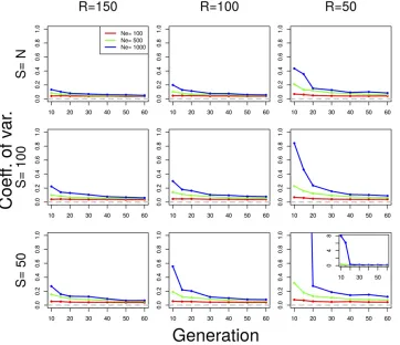
Figure 3 Coefficient of variation ofNeðPÞ under plan I for various parameter values. Neutral Wright–Fisher simulations were performed with various combinations of the parameters: effective population size (Ne¼100; 500; 1000 diploid individu-als), pool size (S¼100;50), and coverage (R¼150; 100; 50). Ne was estimated withNeðPÞunder plan I, usingn¼2000 SNPs.S¼Nindicates scenarios when the whole population is sequenced as a single pool. For all simulations, we assumed

0 andt(Equation 10), which is inversely proportional to the census population size. Consequently, the difference between plans I and II becomes smaller for increasing N. Waples (1989) investigated how the ratio between census and effec-tive population size (r¼N=Ne) affects the accuracy of the estimators and concluded that the ratio ofr$2 is sufficient to reach similar estimates for both sampling schemes. We tested the performance of NeðPÞ on simulated data with

Ne¼100 and N:Ne ratios ofr¼1;2;5 with different cov-erages and pool sizes (Figure S4,Figure S5, andFigure S6). WhenN¼Ne;theNeðPÞplan I method achieves highly accu-rate estimates for all time points in contrast to the other methods (Figure S4). If, however, theNeðPÞplan II estimator is applied to data simulated under plan I, we observe an up-ward bias for small t, which improves with an increasing number of generations. This pattern is not unexpected since the missing covariance term becomes less influential in view of the increasing drift variance after several generations. When the entire population is sequenced as a single pool (S¼100), the plan II estimators of Waples (1989) and Jorde and Ryman (2007) perform similarly to theNeðPÞplan I estimator because the correction for pooling inNeðPÞ can-cels out the additional covariance term whenS¼N;making the term used asFapproximately identical to that ofNeðJRÞ: This is a general pattern irrespective ofr.

Forr$2;NeðPÞplan I remains highly accurate (Figure S5 and Figure S6). Furthermore, when increasing the census size under a constant Ne (equivalent to increasing r), the covariance between sample allele frequencies decreases, making the difference between plans I and II almost negligi-ble (Waples 1989). The sampling variance becomes propor-tionally smaller compared to the drift variance with an increasing number of generations between the samples. This improves our ability to accurately estimateNe:

Correcting for the additional variance inherent to Pool-seq leads to an improved performance ofNeðPÞcompared to the

standard methods for both plans. In general, with Pool-seq data the extent of the bias of theNeðWÞandNeðJRÞestimates depends on the ratio betweenNandS, smaller sample sizes (S) leading to a larger bias. As we accounted for the sequenc-ing step with these estimators (Estimating Ne on simulated

data), decreasing the coverage at a given pool size does not change the bias much but rather increases the variance of the estimators.

In most of the experimental studies the investigator has control over the census population size; thus requiring the knowledge ofNforNeðPÞplan I does not restrict the analysis. We illustrate the performance of NeðPÞ plan I only when

Ne¼N in the main text, but according to Figure S5 and Figure S6,NeðPÞplan I is also highly accurate whenr$2:

We show the coefficient of variation (CV) of theNeðPÞplan I estimator in Figure 3. The CV is defined as the ratio between the standard deviation and the mean (CV¼s^=m^;where both

^

s and m^ are estimated from the sample). It measures the relative dispersion of the distribution of the estimated values.

NeðPÞestimators are highly precise in nearly all cases, except when the drift variance is negligible compared to the sam-pling variance (Figure 3; see alsoFigure S9andFigure S11 whereNe¼1000; t,30; S#100;andR¼50). The bias is coming from a few outlier estimates, but the median shows more robust results (Figure S13). For plan II estimators, the behavior of the method is similar (Figure S8, Figure S10, Figure S12, andFigure S14). Note that the simulations un-derlyingFigure S8,Figure S10,Figure S12, andFigure S14 have been done under plan I.

Increasing the number of SNPs reduces the variance of Ne(P)

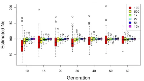
We test how the number of loci (n) used to inferNeaffects the accuracy and the precision of the estimates by gradually in-creasing the number of independent SNPs from 100 to 10,000 (Figure 4). We observe a larger variance and a slight downward bias for a small number of SNPs (100 SNPs). Both the bias and the variance become smaller with a larger

Figure 4 Effect of the number of SNPs used for estimatingNe: The effective population size is estimated usingNeðPÞplan I on simulated data with Ne¼N¼100:A total number ofS¼100 individuals are pooled and sequenced at a mean coverage ofR¼50:Based on 100 simulation runs,Ne is estimated using different numbers of SNPs at multiple time points.

number of SNPs. Some further improvement is obtained when.10,000 SNPs are used (not shown), but the benefit of additional independent SNPs levels off. We conclude that

n¼2000 SNPs usually provide sufficient precision and accu-racy. However, when linkage disequilibrium is present in a genome-wide data set, the number of truly independent SNPs per window is reduced and a larger number of loci is recommended.

A skewed starting allele frequency distribution only moderately increases the variance of Ne(P)

In natural populations, the neutral site frequency spectrum is skewed toward allele frequencies close to the boundaries.

NeðPÞuses a weighting scheme that is not very sensitive to this skew (see also Jorde and Ryman 2007). This makes it robust with respect to the shape of the starting allele fre-quency distribution. We illustrate this with a simulated data set having a starting allele frequency distribution that is skewed toward low- and high-frequency variants (Beta(0.2, 0.2)) as expected under neutrality. The estimates ofNefrom such data sets are compared to simulated data with matching parameters but uniform starting allele frequency distribution (Figure 5). We observe a very slight upward bias with neutral starting allele frequencies compared to uniform and a mod-erate increase in the variance given t$15: With an in-creasing number of generations, the difference becomes negligible.

The presence of linkage disequilibrium does not have a large effect on the precision of Ne(P)

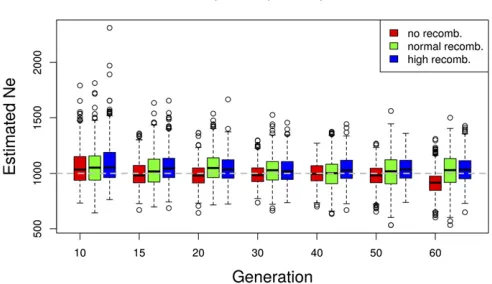
We investigated the sensitivity of our estimator to linkage disequilibrium between loci, using genome-wide neutral sim-ulations with recombination (Kofler and Schlötterer 2014).

We simulated data with three different rates of recombina-tion: high, normal, and no recombination. For thefirst case, the recombination rate is set to mimic the behavior of almost independent SNPs. In the normal recombination rate sce-nario, we use D. melanogasterrecombination rates (Fiston-Lavier et al. 2010). The effective population size was esti-mated in nonoverlapping windows with a fixed number of

n¼10;000 SNPs (Figure 6). Different levels of linkage dis-equilibrium affect the number of independent loci per win-dow. Nevertheless, we observe only a slight increase in the precision of theNeestimates with increasing recombination rate (Figure 6).

HeterogeneousNbe along the genome in an E&R study

with D. melanogaster

We estimatedNein a recent E&R study withD. melanogaster (Orozco-terWengelet al.2012; Franssenet al.2015). In this experiment replicate populations of 1000 individuals were subjected to afluctuating hot environment for 59 generations. Allele frequency estimates were obtained for founder and evolved populations, using Pool-seq.Newas estimated based on the allele frequency changes between founder and latest evolved populations in nonoverlapping windows containing 10,000 SNPs, using NeðPÞ under plan I. To determine the number of DNA stretches with differentNbe along the ge-nome, we use a segmentation algorithm provided in the software tool by Fricket al.(2014). This method requires homogeneity of variances. Since the variance of estimates increases withNe;the estimates were log-transformed before applying the partitioning procedure. The obtained step func-tion was back-transformed to the original scale and is shown for three biological replicates (Figure 7).

The mean and the median estimates for each chromosome arm as well as across the genome are stable across replicates (see Table 1 andTable S1). As experimental evolution stud-ies often aim tofind signals that are consistent across repli-cates, this can be an important check of the experimental setup. On the other hand, we see differences between chro-mosome arms. For example, the mean is clearly lower for 3R, emphasizing the added value of spatial analysis compared to genome-wide estimates.

In D. melanogaster Nbe ranges between 100 and 400. Around the centromere of chromosome 2, the estimatedNe decreases by two-thirds in replicates 1 and 3, which is in agreement with the expectation of low diversity and, as a consequence, lowNein regions with reduced recombination (Begun and Aquadro 1992; Presgraves 2005; Haddrillet al.

2007; Camposet al.2012). Furthermore,Nbe is low on the entire chromosome arm 3R and also on parts of 3L. Overall, these patterns can be attributed to strong LD, caused either by low recombination rates around the centromeres (Chan

et al.2012) or by segregating inversions (Kapunet al.2014) in combination with selection potentially on rare variants. The reduction inNbeis also well captured by the segmentation algorithm (Figure 7), which shows a similar pattern when applied on simulated data with selection (Figure S15). These

results are consistent with those of Tobleret al.(2014), who observed a massive amount of outlier SNPs around the cen-tromere of chromosome 2 and on 3R. Interestingly, certain regions of the genome show extensive differences inNbebetween the replicates, which might be reflecting different selection histories or differences in demography, such as replicate-specific bottlenecks.

b

Nemay also vary as a result of differences in the modes of transmission of different components in the genome. For ex-ample, on the X chromosome,Neis equal to three-quarters of the autosomal population size (Vicoso and Charlesworth 2006, 2009). Interestingly, our estimates in the E&R experi-ment do not reflect this expectation of reduced effective pop-ulation size. Instead, we estimateNeto be as high asNbeon the autosomes. Unequal sex ratio between males and females can be a source of such a pattern (Charlesworth 2009); however, unbalanced sex ratio has not been reported in this experi-ment. Another possible explanation for increasedNbeon the X can be the presence of background selection as suggested by Charlesworth (2012b). He argues that because of the lack of recombination in male Drosophila, the effect of back-ground selection is more effective on the autosomes than on the X chromosome. Orozco-terWengel et al. (2012) re-ported differences in the number of putatively selected sites between the X and autosomes. They found that candidate SNPs were underrepresented on the X. Their selection scan

identifies signatures of deviation from neutral expectation, which is also reflected in the reduction inNbe on the auto-somes, indicating higher selection pressure.

Recommendations for genome-wide data sets

Most of the methods proposed previously are not designed for genome-wide high-density SNP data sets. However, the method of Jorde and Ryman (2007) was successfully used for genome-wide data by Follet al.(2014). Reedet al.(2014) also used a similar approach to estimate Ne for whole-genome data, using sliding windows. We estimatedNein win-dows with afixed number of SNPs. Using windows offixed lengths in base pairs would affect the variance of the estima-tor (Figure 4) but does not disestima-tort the mean. All these ap-proaches, however, do not account for the ruggedness of the recombination landscape and can lead to windows with dif-ferent levels of linkage disequilibrium in them. To overcome this problem it would be possible to define windows based on recombination distance. Unfortunately, the lack of haplotype information in the Pool-seq data makes it difficult to infer linkage disequilibrium. One way to infer linkage information from pooled sequence data is provided by the software LDx (Federet al.2012). For model organisms such asDrosophila, readily available recombination maps can also be used as a proxy (Przeworskiet al.2001; Kulathinalet al.2008; Fiston-Lavieret al.2010). If only a single genome-wideNeestimate

Figure 7 Genome-widebNefrom an E&R study withD. melanogaster.Neis estimated based on the allele frequency changes between founder and evolved populations at generation 59 (Franssen

et al.2015). In the top panel, we show genome-wide estimates calculated withNeðPÞ(plan I), using

is required, one can alternatively use a set of randomly dis-tributed SNPs over the genome to obtainNbe:

Temporal methods make a number of assumptions, which, if violated, can lead to biasedNeestimates. For example, in our simulations, we considered only effective population sizes that are constant over time. FluctuatingNeis a frequent phenomenon in natural populations and can be an important component of an experimental design. For example, in re-peatedly bottlenecked populations, the smallest population size dominatesNbe(Luikartet al.1999; Charlesworth 2009). But even in strictly controlled populations the experimental regime can induce changes in Ne: When the population changes in size, the estimatedNeis generally interpreted as the harmonic mean of the effective population sizes over the generations (Wright 1938; Nei and Tajima 1981; Waples 1989). However, if time series allele frequency data are avail-able, such changes can be detected by estimating Ne from pairwise comparisons between consecutive time points.

All evolutionary forces (selection, demography, etc.) that lead to deviations from the neutral expectation will also affect our estimate. Nevertheless, systematic forces that result in locally different values ofNbecan be detected with a sliding-window approach, as illustrated with simulations under selec-tion (Figure S15). TheD. melanogasterdata set also illustrates this point; i.e., the hypothesized regions under selection co-incide with regions of reduced Ne (Orozco-terWengelet al. 2012; Tobleret al.2014; Franssenet al.2015). For this to be detected, however, most of the allele frequency change has to occur over the sampled time span.

In the E&R study withD. melanogaster, shown above, the criterion of nonoverlapping generations, assumed by tempo-ral methods, is met (see Orozco-terWengel et al. 2012 for details on experimental design). However, for samples from an age-structured population, the resultingNbecan be biased (Waples and Yokota 2007). In these cases, as suggested by Waples and Yokota (2007), larger spacing between samples maximizes the drift signal compared to sampling biases asso-ciated with age structure.

Using a small number of generations can lead to outlier estimates

In general,NeðPÞhas a lower bias but larger variance, espe-cially when tis small. As pointed out by Jorde and Ryman (2007) our weighting scheme leads to an increased variance but a smaller bias compared to other schemes. We observe outlier estimates among replicates at early generations

(gen-eration 5, Figure 2,Figure S4,Figure S5, andFigure S6) for

NeðPÞ:When the sampling variance is large compared to the drift variance (Ne¼1000;S#100;andR¼50;Figure S11 andFigure S12), the deviation of the outlier estimates from the true Ne is particularly large. For a few cases, we even observe large negative estimates. Negative estimates, in gen-eral, can be interpreted asNebeing infinity, that is, no evi-dence of genetic drift (Peelet al.2013). In our simulations this is plausible whenNeis large andtis small, such that drift has not had a large effect on the population allele frequencies yet. Note that the harmonic mean estimator (Nb*eðPÞ) has smaller variance for large Ne (Figure S16). This estimator, however, is less accurate thanNeðPÞfor smallNeas shown inFigure S17.

To eliminate potential outliers and an inflated variance we recommend increasing the signal-to-noise ratio by pooling a sufficient number of individuals. Using later generations or increasing the number of SNPs in the analysis also helps to avoid outlier estimates. When none of these strategies can be applied, we suggest using the genome-wide median NeðPÞ estimates or the harmonic mean estimator, as these are more robust to extreme outliers.

Conclusions

Effective population size is an important parameter for de-scribing evolutionary dynamics, making its accurate estima-tion essential for populaestima-tion genetic studies. Several methods have been designed to estimate Ne;and their performance was comprehensively evaluated on simulated as well as real data (Barker 2011; Serbezovet al.2012; Baalsrudet al.2014; Holleleyet al.2014; Gilbert and Whitlock 2015). These stud-ies mainly focused on genetic data collected from natural populations, which usually differ from experimental studies in terms of the census population size and sampling scheme. We designed a method that accurately infers the effective population size in genome-wide data from experimental populations sequenced in pools. Our approach improves temporal methods by explicitly correcting for two stages of sampling introduced by pooling and sequencing. Our re-sults on simulated data confirm that methods that fail to properly account for the two stages of sampling inherent to Pool-seq can lead to severely biasedNeestimates.

Pool-seq data are often considered to be overdispersed,i.e., displaying more variability than is predicted by the binomial sampling model (Yang et al. 2012). However, Zhu et al.

(2012) and Futschik and Schlötterer (2010) validated that

Table 1 Genome-wide meanNbefrom an E&R study withD. melanogaster

Mean

Replicate X 2L 2R 3L 3R Genome-wide

R1 257.9675 231.6854 257.0828 193.4339 131.7072 199.4463

R2 328.8878 297.9832 274.8529 193.3237 194.9571 239.3618

R3 263.4829 246.5448 211.8995 157.6411 133.9459 187.1573

The effective population size is estimated withNeðPÞplan I in windows of 10,000 SNPs (Figure 7). The mean estimates across windows are shown for the major chromosome

the error in allele frequency estimates is reasonably well ap-proximated by binomial sampling given that a large enough number of individuals are pooled. Nevertheless, if overdis-persion is present in the data, that will lead to additional variance, which is not modeled in our framework and will result in a downward bias of the estimatedNe:If the level of overdispersion can be inferred for the data (see,e.g., Gautier

et al.2013; Illingworth 2015), it is possible to introduce a parameter that accounts for the additional between-pool var-iation (seeFile S1, Equation S8).

We also illustrate the applicability of our method for estimating Ne from experimental data of D. melanogaster and show that in combination with a recursive partitioning method we can infer patterns of local variation inNealong the genome. Additionally, it is possible to calculate confi -dence intervals based on thex2 _{distribution (Waples 1989)} or alternatively apply a nonparametric bootstrap approach.

Software availability

Our proposed estimators along with standard methods from the literature are implemented within the R packageNest. The package is currently available at https://github.com/Tho-masTaus/Nest.

Acknowledgments

We thank Mads Fristrup Schou, Susanne U. Franssen, and Neda Barghi for helpful comments on the Nest software package and Robin S. Waples and an anonymous reviewer for their constructive comments that greatly improved the manuscript. A.J. and T.T. are members of the Vienna Grad-uate School of Population Genetics, which is funded by the Austrian Science Fund (FWF, W1225). C.S. is also supported by the European Research Council grant ”ArchAdapt,”and T.T. is a recipient of a Doctoral Fellowship (DOC) of the Austrian Academy of Sciences.

Literature Cited

Anderson, E. C., E. G. Williamson, and E. A. Thompson, 2000 Monte Carlo evaluation of the likelihood for N(e) from temporally spaced samples. Genetics 156(4): 2109_–2118. Baalsrud, H. T., B.-E. Saether, I. J. Hagen, A. M. Myhre, T. H.

Ringsby et al., 2014 Effects of population characteristics and structure on estimates of effective population size in a house sparrow metapopulation. Mol. Ecol. 23(11): 2653– 2668.

Barker, J. S. F., 2011 Effective population size of natural popula-tions ofDrosophila buzzatii, with a comparative evaluation of nine methods of estimation. Mol. Ecol. 20(21): 4452–4471. Barrick, J. E., D. S. Yu, S. H. Yoon, H. Jeong, T. K. Oh et al.,

2009 Genome evolution and adaptation in a long-term exper-iment withEscherichia coli. Nature 461(7268): 1243–1247. Barton, N. H., 2000 Genetic hitchhiking. Philos. Trans. R. Soc.

Lond. B Biol. Sci. 355(1403): 1553–1562.

Bastide, H., A. Betancourt, V. Nolte, R. Tobler, P. Stöbe et al., 2013 A genome-wide,_fine-scale map of natural pigmentation variation in Drosophila melanogaster. PLoS Genet. 9(6): e1003534.

Baysal, B. E., E. C. Lawrence, and R. E. Ferrell, 2007 Sequence variation in human succinate dehydrogenase genes: evidence for long-term balancing selection on SDHA. BMC Biol. 5: 12. Begun, D. J., and C. F. Aquadro, 1992 Levels of naturally

occur-ring DNA polymorphism correlate with recombination rates in

D. melanogaster. Nature 356(6369): 519–520.

Berry, A. J., J. W. Ajioka, and M. Kreitman, 1991 Lack of poly-morphism on theDrosophilafourth chromosome resulting from selection. Genetics 129: 1111–1117.

Boitard, S., R. Kofler, P. Françoise, D. Robelin, C. Schlöttereret al., 2013 Pool-hmm: a Python program for estimating the allele frequency spectrum and detecting selective sweeps from next generation sequencing of pooled samples. Mol. Ecol. Resour. 13 (2): 337–340.

Burke, M. K., J. P. Dunham, P. Shahrestani, K. R. Thornton, M. R. Roseet al., 2010 Genome-wide analysis of a long-term evolu-tion experiment withDrosophila. Nature 467(7315): 587_–590. Burke, M. K., G. Liti, and A. D. Long, 2014 Standing genetic var-iation drives repeatable experimental evolution in outcrossing populations ofSaccharomyces cerevisiae. Mol. Biol. Evol. 31(12): 3228_–3239.

Campos, J. L., B. Charlesworth, and P. R. Haddrill, 2012 Molecular evolution in nonrecombining regions of the

Drosophila melanogaster genome. Genome Biol. Evol. 4(3): 278–288.

Chan, A. H., P. A. Jenkins, and Y. S. Song, 2012 Genome-wide

fine-scale recombination rate variation in Drosophila mela-nogaster. PLoS Genet. 8(12): e1003090.

Charlesworth, B., 1996 Background selection and patterns of ge-netic diversity in Drosophila melanogaster. Genet. Res. 68(2): 131–149.

Charlesworth, B., 2009 Fundamental concepts in genetics: effec-tive population size and patterns of molecular evolution and variation. Nat. Rev. Genet. 10(3): 195–205.

Charlesworth, B., 2012a The effects of deleterious mutations on evolution at linked sites. Genetics 190(1): 5–22.

Charlesworth, B., 2012b The role of background selection in shaping patterns of molecular evolution and variation: evidence from variability on theDrosophilaX chromosome. Genetics 191: 233_–246.

Comeron, J. M., A. Williford, and R. M. Kliman, 2008 The Hill-Robertson effect: evolutionary consequences of weak selection and linkage in_finite populations. Heredity 100(1): 19_–31. Excof_fier, L., and M. Foll, 2011 Fastsimcoal: a continuous-time

coalescent simulator of genomic diversity under arbitrarily com-plex evolutionary scenarios. Bioinformatics 27(9): 1332_–1334. Falconer, D. S., and T. F. C. Mackay, 1996 Introduction to

Quan-titative Genetics. Benjamin-Cummings, Menlo Park, CA. Feder, A. F., D. A. Petrov, and A. O. Bergland, 2012 LDx:

estima-tion of linkage disequilibrium from high-throughput pooled re-sequencing data. PLoS One 7(11): e48588.

Ferretti, L., S. E. Ramos-Onsins, and M. Pérez-Enciso, 2013 Population genomics from pool sequencing. Mol. Ecol. 22(22): 5561–5576. Fisher, R., 1930 The Genetical Theory of Natural Selection. Oxford

University Press, Oxford.

Fiston-Lavier, A.-S., N. D. Singh, M. Lipatov, and D. A. Petrov, 2010 Drosophila melanogaster recombination rate calculator. Gene 463(1–2): 18–20.

Foll, M., Y.-P. Poh, N. Renzette, A. Ferrer-Admetlla, C. Banket al., 2014 Influenza virus drug resistance: a time-sampled popula-tion genetics perspective. PLoS Genet. 10(2): e1004185. Foll, M., H. Shim, and J. D. Jensen, 2015 WFABC: a Wright-Fisher

ABC-based approach for inferring effective population sizes and selection coefficients from time-sampled data. Mol. Ecol. Resour. 15(1): 87_–98.

evolving experimental Drosophila melanogasterpopulations. Mol. Biol. Evol. 32(2): 495–509.

Frick, K., A. Munk, and H. Sieling, 2014 Multiscale change point inference. J. R. Stat. Soc. Ser. B Stat. Methodol. 76(3): 495–580. Futschik, A., and C. Schlötterer, 2010 The next generation of mo-lecular markers from massively parallel sequencing of pooled DNA samples. Genetics 186(1): 207–218.

Futschik, A., T. Hotz, A. Munk, and H. Sieling, 2014 Multiscale DNA partitioning: statistical evidence for segments. Bioinfor-matics 30(16): 2255–2262.

Gautier, M., J. Foucaud, K. Gharbi, T. Cézard, M. Galan et al., 2013 Estimation of population allele frequencies from next-generation sequencing data: pool-vs.individual-based genotyp-ing. Mol. Ecol. 22(14): 3766–3779.

Gilbert, K. J., and M. C. Whitlock, 2015 Evaluating methods for estimating local effective population size with and without mi-gration. Evolution 69(8): 2154_–2166.

Haddrill, P. R., D. L. Halligan, D. Tomaras, and B. Charlesworth, 2007 Reduced ef_ficacy of selection in regions of theDrosophila

genome that lack crossing over. Genome Biol. 8(2): R18. Hill, W. G., 1981 Estimation of effective population size from data

on linkage disequilibrium. Genet. Res. 38: 209–216.

Holleley, C. E., R. A. Nichols, M. R. Whitehead, A. T. Adamack, M. R. Gunn et al., 2014 Testing single-sample estimators of effective population size in genetically structured populations. Conserv. Genet. 15: 23–35.

Huang, Y., S. I. Wright, and A. F. Agrawal, 2014 Genome-wide patterns of genetic variation within and among alternative se-lective regimes. PLoS Genet. 10(8): e1004527.

Hui, T.-Y. J., and A. Burt, 2015 Estimating effective population size from temporally spaced samples with a novel, efficient max-imum-likelihood algorithm. Genetics 200: 285–293.

Illingworth, C. J. R., 2015 Fitness inference from short-read data: within-host evolution of a reassortant H5N1 influenza virus. Mol. Biol. Evol. 32(11): 3012–3026.

Jorde, P. E., and N. Ryman, 2007 Unbiased estimator for genetic drift and effective population size. Genetics 177: 927–935. Kapun, M., H. van Schalkwyk, B. McAllister, T. Flatt, and C.

Schlöt-terer, 2014 Inference of chromosomal inversion dynamics from Pool-Seq data in natural and laboratory populations of

Drosophila melanogaster. Mol. Ecol. 23(7): 1813_–1827. Kawecki, T. J., R. E. Lenski, D. Ebert, B. Hollis, I. Olivieri et al.,

2012 Experimental evolution. Trends Ecol. Evol. 27(10): 547_–560. Kimura, M., 1964 Diffusion model in population genetics. J. Appl.

Probab. 1: 177_–223.

Kimura, M., and J. F. Crow, 1963 The measurement of effective population number. Evolution 17(3): 279–288.

Kofler, R., and C. Schlötterer, 2014 A guide for the design of evolve and resequencing studies. Mol. Biol. Evol. 31(2): 474–483. Kofler, R., P. Orozco-terWengel, N. De Maio, R. V. Pandey, V. Nolte

et al., 2011a PoPoolation: a toolbox for population genetic analysis of next generation sequencing data from pooled indi-viduals. PLoS One 6(1): e15925.

Kofler, R., R. V. Pandey, and C. Schlötterer, 2011b PoPoolation2: identifying differentiation between populations using sequenc-ing of pooled DNA samples (Pool-Seq). Bioinformatics 27(24): 3435–3436.

Kolaczkowski, B., A. D. Kern, A. K. Holloway, and D. J. Begun, 2011 Genomic differentiation between temperate and tropical Australian populations of Drosophila melanogaster. Genetics 187: 245–260.

Krimbas, C. B., and S. Tsakas, 1971 The genetics ofDacus oleae. V. Changes of esterase polymorphism in a natural population fol-lowing insecticide control – Selection or drift? Evolution 25: 454_–460.

Kulathinal, R. J., S. M. Bennett, C. L. Fitzpatrick, and M. A. F. Noor, 2008 Fine-scale mapping of recombination rate inDrosophila

refines its correlation to diversity and divergence. Proc. Natl. Acad. Sci. USA 105(29): 10051–10056.

Liu, Y., and J. E. Mittler, 2008 Selection dramatically reduces effective population size in HIV-1 infection. BMC Evol. Biol. 8: 133.

Long, A., G. Liti, A. Luptak, and O. Tenaillon, 2015 Elucidating the molecular architecture of adaptation via evolve and rese-quence experiments. Nat. Rev. Genet. 16(10): 567–582. Luikart, G., J. M. Cornuet, and F. W. Allendorf, 1999 Temporal

changes in allele frequencies provide estimates of population bottleneck size. Conserv. Biol. 13(3): 523–530.

Maynard Smith, J., and J. Haigh, 1974 The hitch-hiking effect of a favourable gene. Genet. Res. 23: 23–35.

Nei, M., and F. Tajima, 1981 Genetic drift and estimation of ef-fective population size. Genetics 98: 625_–640.

Nomura, T., 2008 Estimation of effective number of breeders from molecular coancestry of single cohort sample. Evol. Appl. 1(3): 462_–474.

Orozco-terWengel, P., M. Kapun, V. Nolte, R. Ko_fler, T. Flattet al., 2012 Adaptation ofDrosophilato a novel laboratory environ-ment reveals temporally heterogeneous trajectories of selected alleles. Mol. Ecol. 21(20): 4931–4941.

Pamilo, P., and S. L. Varvio-Aho, 1980 On the estimation of popula-tion size from allele frequency changes. Genetics 95: 1055–1057. Peel, D., R. S. Waples, G. M. Macbeth, C. Do, and J. R. Ovenden,

2013 Accounting for missing data in the estimation of contem-porary genetic effective population size (N(e)). Mol. Ecol. Re-sour. 13(2): 243–253.

Pollak, E., 1983 A new method for estimating the effective pop-ulation size from allele frequency changes. Genetics 104: 531– 548.

Presgraves, D. C., 2005 Recombination enhances protein adapta-tion inDrosophila melanogaster. Curr. Biol. 15(18): 1651–1656. Przeworski, M., J. D. Wall, and P. Andolfatto, 2001 Recombination and the frequency spectrum inDrosophila melanogasterand Dro-sophila simulans. Mol. Biol. Evol. 18(3): 291–298.

Pudovkin, A. I., D. V. Zaykin, and D. Hedgecock, 1996 On the potential for estimating the effective number of breeders from heterozygote-excess in progeny. Genetics 144: 383–387. Reed, L. K., K. Lee, Z. Zhang, L. Rashid, A. Poe et al.,

2014 Systems genomics of metabolic phenotypes in wild-type

Drosophila melanogaster. Genetics 197: 781_–793.

Schlötterer, C., R. Tobler, R. Ko_fler, and V. Nolte, 2014 Sequencing pools of individuals - mining genome-wide polymorphism data without big funding. Nat. Rev. Genet. 15(11): 749_–763. Schlötterer, C., R. Kofler, E. Versace, R. Tobler, and S. U. Franssen,

2015 Combining experimental evolution with next-generation sequencing: a powerful tool to study adaptation from standing genetic variation. Heredity 114(5): 431–440.

Serbezov, D., P. E. Jorde, L. Bernatchez, E. M. Olsen, and L. A. Vllestad, 2012 Short-term genetic changes: evaluating effec-tive population size estimates in a comprehensively described brown trout (Salmo trutta) population. Genetics 191: 579–592. Tallmon, D. A., A. Koyuk, G. Luikart, and M. A. Beaumont, 2008 Computer Programs: onesamp: a program to estimate effective population size using approximate Bayesian computa-tion. Mol. Ecol. Resour. 8(2): 299–301.

Tobler, R., S. U. Franssen, R. Kofler, P. Orozco-terWengel, V. Nolte

et al., 2014 Massive habitat-specific genomic response inD. melanogasterpopulations during experimental evolution in hot and cold environments. Mol. Biol. Evol. 31(2): 364–375. Turner, T. L., and P. M. Miller, 2012 Investigating natural

varia-tion inDrosophilacourtship song by the evolve and resequence approach. Genetics 191: 633–642.

Turner, T. L., A. D. Stewart, A. T. Fields, W. R. Rice, and A. M. Tarone, 2011 Population-based resequencing of experimen-tally evolved populations reveals the genetic basis of body size variation in Drosophila melanogaster. PLoS Genet. 7(3): e1001336.

Vicoso, B., and B. Charlesworth, 2006 Evolution on the X chro-mosome: unusual patterns and processes. Nat. Rev. Genet. 7: 645–653.

Vicoso, B., and B. Charlesworth, 2009 Effective population size and the faster-X effect: an extended model. Evolution 63(9): 2413_–2426.

Wang, J., 2001 A pseudo-likelihood method for estimating effec-tive population size from temporally spaced samples. Genet. Res. 78(3): 243_–257.

Wang, J., 2009 A new method for estimating effective population sizes from a single sample of multilocus genotypes. Mol. Ecol. 18(10): 2148–2164.

Wang, J., 2013 A simulation module in the computer program COLONY for sibship and parentage analysis. Mol. Ecol. Resour. 13(4): 734–739.

Waples, R. S., 1989 A generalized approach for estimating effec-tive population size from temporal changes in allele frequency. Genetics 121: 379–391.

Waples, R. S., and C. Do, 2008 LDNe: a program for estimating effective population size from data on linkage disequilibrium. Mol. Ecol. Resour. 8(4): 753–756.

Waples, R. S., and C. Do, 2010 Linkage disequilibrium estimates of contemporary Ne using highly variable genetic markers: a largely untapped resource for applied conservation and evolu-tion. Evol. Appl. 3(3): 244–262.

Waples, R. S., and P. R. England, 2011 Estimating contemporary effective population size on the basis of linkage disequilibrium in the face of migration. Genetics 189: 633–644.

Waples, R. S., and M. Yokota, 2007 Temporal estimates of effec-tive population size in species with overlapping generations. Genetics 175: 219–233.

Williamson, E. G., and M. Slatkin, 1999 Using maximum likeli-hood to estimate population size from temporal changes in al-lele frequencies. Genetics 152: 755_–761.

Wright, S., 1931 Evolution in Mendelian populations. Genetics 16: 97–159.

Wright, S., 1938 Size of population and breeding structure in re-lation to evolution. Science 87: 430–431.

Yang, X., J. A. Todd, D. Clayton, and C. Wallace, 2012 Extra-binomial variation approach for analysis of pooled DNA sequenc-ing data. Bioinformatics 28(22): 2898–2904.

Zhu, Y., A. O. Bergland, J. González, and D. A. Petrov, 2012 Empirical validation of pooled whole genome population re-sequencing in Drosophila melanogaster. PLoS One 7(7): e41901.

Supplement

´

Agnes J´

on´

as, Thomas Taus, Carolin Kosiol, Christian Schl¨

otterer, Andreas Futschik

1

Normalized allele frequency changes under two-step

sam-pling

1.1

Calculating the expected normalized variation

In the following, we calculate the expected value for a measure of allele frequency change due to

the combination oftgenerations of drift and sampling. As in Waples (1989), we consider

Fc =

Pa

i=1(ˆxk−yˆk)2 Pa

k=1zˆk−xˆkyˆk

, (S1)

as our measure, where ˆxand ˆy denote the observed allele frequencies in the pooled DNA sample

collected t generations apart, a is the number of alleles at a locus and ˆzk := (ˆxk+ ˆyk)/2. We

consider only biallelic sites, which reduces equation (S1) to

Fc=

(ˆx−y)ˆ 2

ˆ

z−ˆxˆy (S2)

for a given locus. The expectation ofFc is approximated in the following way:

E(Fc)≈

E(ˆx−y)ˆ 2 E(ˆz−xˆˆy) =

V ar(ˆx) +V ar(ˆy)−2Cov(ˆx,y)ˆ

E(ˆz−xˆˆy) . (S3)

We will provide expressions for the numerator and denominator in equation (S3) both for plan I and II under the two-step sampling process. For this purpose, we introduce the following notation: Let

pandptdenote the true allele frequency in the gamete pool preceding the first sampled generation

(0) and aftertgenerations, respectively. S0 is the number of individuals sampled at the first time

point (generation 0), and x denotes the relative allele frequency in this sample. As in the main

text, we distinguish between the allele frequencies (x, y) estimated after sampling individuals at

generations 0 andt, and the frequencies (ˆx,y) after pool sequencing based onˆ Rj (j∈ {0, t}) reads.

For a visual representation of our sampling schemes along with the notation see Fig. S1.

We refer to previous findings of Waples (1989) without carrying out the detailed derivations here, namely

1. The variance ofxis binomial under both plans:

V ar(x) =E(x−p)2=p(1−p)

2S0

. (S4)

2. The variance due totgenerations of genetic drift is:

V ar(pt|p) =E(pt−p)2=p(1−p) "

1−

1− 1

2Ne

t#

. (S5)

We consider the relevant terms in eq. (S3) separately:

V ar(ˆx) =E(V ar(ˆx|x)) +V ar(E(ˆx|x))

=E

_x(1−x)

R0

+V ar(x|p)

= 1

R0[p−E((x−p+p)

2_{)] +}p(1−p) 2S0

= 1

R0[p−p

2

−E(x−p)2] +p(1−p) 2S0

= 1

R0[p(1−p)−V ar(x)] +

p(1−p)

2S0

= 1

R0

p(1−p)−p(1−p)

2S0

+p(1−p)

2S0

=p(1−p)

₁ 2S0 + 1 R0 − 1 2S0R0 .

Note that we assume a diploid population with sample size of 2S0 and effective population size of

2Ne. Replacing 2S0 with S0 leads to the variance of ˆxin a haploid population with effective size

Ne. We now derive the variance of the sample allele frequency atT =t.

V ar(ˆy) =E(V ar(ˆy|y)) +V ar(E(ˆy|y))

=E

y(1−y)

Rt

+V ar(y|p)

= 1

Rt

(p−E(y−p+p)2) +V ar(y|p)

= 1

Rt

(p−p2−V ar(y|p)) +V ar(y|p)

= 1

Rt "

p(1−p)−p(1−p)

"

1−

1− 1

2Ne

t

1− 1

2St

##

+p(1−p)

"

1−

1− 1

2Ne

t

1− 1

2St

#

=p(1−p)

" 1 Rt − 1 Rt " 1−

1− 1

2Ne

t

1− 1

2St # + " 1−

1− 1

2Ne

t

1− 1

2St

##

=p(1−p)

"

1−

1− 1

Rt

1− 1

2St

1− 1

2Ne

t#

Here, 2Sj is the number of sampled chromosomes in a diploid population at time t. For a haploid

population, the factor 2 can be ignored for both the sample size and the effective population size.

We introduce a correction term Cj := _2S1 j +

1

Rj −

1

2SjRj for Fc at generationsj ∈ {0, t}. For

haploid populations an analogous correction term isCj(hapl.):= _S1_j +_R1_j −_Sj1_Rj (j∈ {0, t}). Based

on the results above, the variance in sample allele frequency atT = 0 andt can be written as

V ar(ˆx) =p(1−p)C0 , (S6)

and

V ar(ˆy) =p(1−p)

"

1−(1−Ct)

1− 1

2Ne

t#

. (S7)

In the haploid case, we haveV ar(ˆy) =p(1−p)

1−(1−Ct(hapl.))

1− 1

Ne

t

.

Pool-seq data can be over-dispersed, e.g. if different individuals in the pool have different

probabilities of contributing the sequenced reads.

If the level of overdispersion can be inferred from the data, then it is possible to account for

the additional variance by introducing an overdispersion parameter γ. This parameter can be

interpreted as the factor by which the actual variance exceeds the theoretical binomial variance.

Withγ, our correction term becomes

Cj(disp.)= 1

2Sj

+ γ

Rj

− γ

2SjRj

. (S8)

Following Waples (1989) the denominator in equation (S3) reduces to

E(ˆz−xˆˆy) =p(1−p)−Cov(ˆx,y)ˆ . (S9)

We now investigate the covariance term separately for both sampling plans.

1.2

Sampling plan II

Under sampling plan II, a sample of sizeS0 is taken before reproduction and is not replaced in the

population. Consequenty, the sample ofS0 individuals and the 2Ne chromosomes contributing to

the next generation are mutually exclusive, implying that the sample allele frequency at generation

0 is uncorrelated to the sample allele frequency att, i.e.Cov(ˆx,y) = 0 for sampling plan II. We nowˆ

plug equations (S6), (S7), and (S9) into equation (S3). With equation (S7), we use the equation (2) from the main text.

E(Fc)≈

V ar(ˆx) +V ar(ˆy)−2Cov(ˆx,y)ˆ p(1−p)−Cov(ˆx,y)ˆ

= V ar(ˆx) +V ar(ˆy)

p(1−p)

= p(1−p)C0+p(1−p)

1−(1−Ct)e−t/2Ne

p(1−p)

=C0+ 1−e−t/2Ne+Cte−t/2Ne

=C0+ 1−e−t/2Ne_−C

t(1−e−t/2Ne) +Ct

=C0+Ct+ (1−Ct)(1−e−t/2Ne)

By solving this equation and replacingE(Fc) byFc, under plan II we obtain a measure of variance

corrected for the two-step sampling

F_c0= Fc−C0−Ct

1−Ct

. (S10)

The effective population size can then be estimated using the method of moments, i.e. equating

F_c0 =E[F_c0] and solving for Ne.

1.3

Sampling plan I

Under sampling plan I, a sample ofS0 individuals is taken after reproduction, so the sample will

contain chromosomes that might contribute to the next generation. This implies that the sample

allele frequency at generation 0 is positively correlated with the sample allele frequency at t, i.e.

Cov(ˆx,y)ˆ >0, because both are derived from the same initial sample at generation 0. Note that

the covariance in equation (S3) would be zero, if the allele frequencyp0of this initial sample were

known because sampling itself at the two time points are independent. Similar to Waples (1989),

it can be shown that the covariance of ˆxand ˆy is simply the variance ofp0. Indeed

ˆ

x=p+ (p0−p) + (x−p0) + (ˆx−x) =p0+ (ˆx−p0), (S11)

and

ˆ

y=p+ (p0−p) + (pt−p0) + (y−pt) + (ˆy−y) =p0+ (ˆy−p0). (S12)

Thus

Cov(ˆx,y) =ˆ V ar(p0) =E(p0−p)2= p(1−p)

2N , (S13)

withN denoting the number of diploid individuals in the initial population, andpis the true allele

frequency in the gamete pool preceding generation 0. This leads to the following estimate ofE(Fc)

for plan I

E(Fc)≈

V ar(ˆx) +V ar(ˆy)−2Cov(ˆx,y)ˆ p(1−p)−Cov(ˆx,y)ˆ

= p(1−p)C0+p(1−p)

1−(1−Ct)e−t/2Ne−2p(1₂−_Np)

p(1−p)−p(1₂−_Np)

= C0+ 1−e

−t/2Ne_+C

te−t/2Ne−_N1

1− 1

2N

= C0+ (1−e

−t/2Ne_)−C

t(1−e−t/2Ne) +Ct−N1

1− 1

2N

= C0+Ct+ (1−e

−t/2Ne_)(1−C t)−_N1

1− 1

2N

ReplacingE(Fc) byFc leads to the corrected estimator ofF under plan I

F_c0 =Fc 1− 1 2N

−C0−Ct+N1

1−Ct

. (S14)

As under plan II, a method of moments estimator can now be computed usingF0

c. Note that for

haploid populations, the covariance in eq. (S13) reduces toCov(ˆx,y) =ˆ p(1_N−p), and eq. (S14) for

haploids will beF_c0= Fc(1−

1

N)−C0(hapl.)−Ct(hapl.)+N2

1−Ct(hapl.) .

References

H. Bastide, A. Betancourt, V. Nolte, R. Tobler, P. St¨obe, A. Futschik, and C. Schl¨otterer. A

genome-wide, fine-scale map of natural pigmentation variation inDrosophila melanogaster. PLoS

Genet, 9(6):e1003534, Jun 2013. doi: 10.1371/journal.pgen.1003534. URLhttp://dx.doi.org/

10.1371/journal.pgen.1003534.

A. Futschik, T. Hotz, A. Munk, and H. Sieling. Multiscale dna partitioning: statistical evidence

for segments.Bioinformatics, 30(16):2255–2262, Aug 2014. doi: 10.1093/bioinformatics/btu180.

URLhttp://dx.doi.org/10.1093/bioinformatics/btu180.

P. E. Jorde and N. Ryman. Unbiased estimator for genetic drift and effective population size.

Genetics, 177(2):927–935, Oct 2007. doi: 10.1534/genetics.107.075481. URL http://dx.doi.

org/10.1534/genetics.107.075481.

R. Kofler and C. Schl¨otterer. A guide for the design of evolve and resequencing studies. Mol Biol

Evol, 31(2):474–483, Feb 2014. doi: 10.1093/molbev/mst221. URL http://dx.doi.org/10.

1093/molbev/mst221.

M. Nei and F. Tajima. Genetic drift and estimation of effective population size. Genetics, 98(3):

625–640, Jul 1981.

Figure S1: Two-step sampling schemes. We follow the sampling schemes proposed by Nei and Tajima (1981) and generalized by Waples (1989). Under sampling scheme I (plan I) a sample is taken after reproduction. Under the second scheme (plan II), the sample is taken before reproduction and is not returned to the population, so the sampled individuals and the ones contributing to the next generation are mutually exclusive (Waples, 1989). Allele frequencies are obtained after a

two-step sampling process: First a sample ofSj (j ∈ {0, t}) individuals is taken to create a pooled

library for DNA extraction (green), that is subjected to high throughput sequencing. SamplingRj

(j ∈ {0, t}) reads is modeled in the second step (red). At each step the relative allele frequencies

in the corresponding samples are indicated under the circles representing the sample. This is a modified version of a figure in Waples (1989).