Spatial Regression Analysis of Pedestrian Crashes Based on Point of Interest Data

ISSN Online: 2327-7203 ISSN Print: 2327-7211

DOI: 10.4236/jdaip.2020.81001 Dec. 17, 2019 1 Journal of Data Analysis and Information Processing

Spatial Regression Analysis of Pedestrian

Crashes Based on Point-of-Interest Data

Yanyan Chen, Jiajie Ma, Shaohua Wang

College of Metropolitan Transportation, Beijing University of Technology, Beijing, China

Abstract

Pedestrian safety has recently been considered as one of the most serious is-sues in the research of traffic safety. This study aims at analyzing the spatial correlation between the frequency of pedestrian crashes and various predictor variables based on open source point-of-interest (POI) data which can pro-vide specific land use features and user characteristics. Spatial regression models were developed at Traffic Analysis Zone (TAZ) level using 10,333 pe-destrian crash records within the Fifth Ring of Beijing in 2015. Several spatial econometrics approaches were used to examine the spatial autocorrelation in crash count per TAZ, and the spatial heterogeneity was investigated by a geo-graphically weighted regression model. The results showed that spatial error model performed better than other two spatial models and a traditional ordi-nary least squares model. Specifically, bus stops, hospitals, pharmacies, res-taurants, and office buildings had positive impacts on pedestrian crashes, while hotels were negatively associated with the occurrence of pedestrian crashes. In addition, it was proven that there was a significant sign of locali-zation effects for different POIs. Depending on these findings, lots of recom-mendations and countermeasures can be proposed to better improve the traf-fic safety for pedestrians.

Keywords

Pedestrian Crashes, Traffic Analysis Zone (TAZ), Spatial Econometrics Approaches, Geographically Weighted Regression, Transportation Safety Planning

1. Introduction

Traffic safety has recently been considered as one of the greatest issues in urban management worldwide. Due to the influencing factors from different aspects,

How to cite this paper: Chen, Y.Y., Ma, J.J. and Wang, S.H. (2020) Spatial Regres-sion Analysis of Pedestrian Crashes Based on Point-of-Interest Data. Journal of Data Analysis and Information Processing, 8, 1-19.

https://doi.org/10.4236/jdaip.2020.81001

Received: October 31, 2019 Accepted: December 14, 2019 Published: December 17, 2019

Copyright © 2020 by author(s) and Scientific Research Publishing Inc. This work is licensed under the Creative Commons Attribution International License (CC BY 4.0).

DOI: 10.4236/jdaip.2020.81001 2 Journal of Data Analysis and Information Processing traffic crashes caused a huge loss in the economy and people’s happiness. It is reported that around 1.35 million people die on the world’s roads each year [1]. Road traffic injuries are the leading killer to people of 5 - 29 years of age, who are almost children and young adults. Even worse, approximately 23% of global road traffic deaths are pedestrians, who are still undervalued in road traffic sys-tem design in many countries. As we can see, there is a great gap between the current situation and safety target in the future. Pedestrians have no protection of vehicle body, seatbelt and so on, so they get direct strike in road accidents, facing more serious injury. If pedestrians were involved in accidents, the fatality risk increases about 3.7 times [2]. With rapid urbanization and motorization, the number of pedestrian crashes in China has increased a lot in the past few years.

In order to capture contributing factors for pedestrian crashes, their locations are usually aggregated into different spatial units [3], such as segments, intersec-tions, mid-blocks, corridors, zones and so on. Many studies have conducted the safety analysis of pedestrian crashes based on zone-level data and examined a lot of related features. A spatial analysis effectively allows for identifying spatial dis-tributions and trends in a larger area, which could help establish long-term planning schemes to improve pedestrians’ safety. Since crash occurrences are not independent across space, pedestrian crash risk may vary significantly in different urban areas. It has been shown that spatial autocorrelation and spatial heterogeneity in crash data are two critical properties when developing statistical models for macro-level safety analysis. Fortunately, important improvements in analytic methods facilitate procedures of safety research on pedestrian crashes. Geographic information system (GIS) is powerful platform supporting lots of spatial regression models. GeoDa software adopted in many recent studies can be used to establish Bayesian models on spatial correlation. The reproducibility of using R language to perform spatial data analysis is unparalleled, which in-cludes plenty of spatial packages for different purposes.

Pedestrian crash occurrences are correlated with various kinds of attributes, such as land use, vehicle kilometers traveled, road features, traffic volume, so-cio-demographic characteristics and so forth. However, the accuracy and relia-bility of these data can hardly be assured. Besides, the unavailarelia-bility is another concern; the sources are not open for the public by relevant authorities. Instead, point-of-interest (POI) data from anywhere in the world can be collected with help of web scraping and other open sources. Although POI data may not in-clude traditional information used in traffic accident analysis, they can represent specific land use factors with precise locations, which are expected to be highly related to pedestrian crashes in both macro- and micro-level aspects. Addition-ally, making good use of POI data may be effective in practice, for instance, as an assistance for transportation planning.

DOI: 10.4236/jdaip.2020.81001 3 Journal of Data Analysis and Information Processing crashes in different regions based on POI data. Section 2 presents a review of previous research on crash spatial analysis, including different perspectives, me-thods and types of traffic crashes. Section 3 narrates the data used in this study: pedestrian crash data and POI data are statistically described, and crash count for each spatial unit is visualized. Section 4 focuses on the methodology in two ways: ordinary least squares (OLS) regression model, spatial lag model (SLM), spatial error model (SEM) and spatial Durbin model (SDM) are introduced to deal with the spatial dependence in data, and geographically weighted regression (GWR) model is developed for analyzing the spatial heterogeneity. In Section 5, results of established models are presented, spatial characteristics are analyzed, and differences between different models are compared. In Section 6, conclu-sions of this study are provided, and relative measures for safety improving are recommended to policy makers.

2. Literature Review

In order to find out the contributing factors for pedestrian crashes, a lot of ap-proaches have been proposed. Some researchers used statistical analysis to mod-el accident frequency [4] [5] [6]. There are also studies focusing the accident in-jury severity [7] [8] [9] [10] [11]. However, spatial and temporal attributes of ac-cident data are considered by many researchers all the time [12]-[17]. From a macro scale, accident distribution characteristics can be depicted by spatially clustering methods. Using time series models, we can recognize the trend and seasonality of accident occurrence in one certain place.

An accident’s location is always an important factor, which can be used for identifying black spots. In many existing studies, kernel density estimation (KDE) is a very common method for identifying gatherings of traffic crashes. The KDE method has two branches specifically: one is the planar KDE [18] [19] [20]; and another is network KDE [21] [22] [23]. Planar KDE can provide a whole-scale view of black spots of traffic accidents. However, considering that traffic accidents mostly take place along roads and streets, a network KDE is more appropriate. Distribution of pedestrian crashes in the research area can al-so be realized by the KDE method, which can merge single crash points into continuous hazardous area [24] [25].

DOI: 10.4236/jdaip.2020.81001 4 Journal of Data Analysis and Information Processing correlation with the crash number.

Spatial dependence is prevalent in traffic crash data, which can be tested by two spatial statistical methods: Moran’s I and Getis-Ord Gi* [32]. In fact, Mo-ran’s I is for global spatial autocorrelation test, while Getis-Ord Gi* is for local spatial autocorrelation test. Besides, spatial econometrics approaches were used for analyzing road accidents in a number of studies. Based on the smallest ad-ministrative divisions, Simões used spatial autoregressive model (SAR), spatial error model (SEM) to analyze traffic accidents with victims in Lisbon [33]. They also tried different space weight matrices (Queen’s case, K Nearest Neighbor, Minimum Distance), but in all cases no spatial autocorrelation was detected.

Rhee et al. made a spatial research on traffic crashes at the traffic analysis zone

(TAZ) level [31]. The results showed SEM model outperformed both SAR model and ordinary least squares (OLS). They also concluded that road speed limit, number of residents, vehicle kilometers of travel were associated with the

num-ber of accidents. Combined crash data with POI data, Jia et al. developed two

spatial regression models [29]. They found that the performance of spatial lag model (SLM) and spatial error model (SEM) were even close, and bank density and hospital density had significantly positive impacts on road accidents.

There are also a group of studies using conditional autoregressive (CAR) to analyze crashes from different perspectives. Kaplan and Prato focused on the frequency and severity of bicycle accidents occurred on the Copenhagen Region [34]. The findings illustrated that the number of crashes and the increase in the

average bicycle daily traffic have a non-linear relation. Xie et al. developed a

multivariate CAR model to model crash counts by injury severity in considera-tion of spatial autocorrelaconsidera-tion [27]. The results showed that their model was able

to capture the spatial autocorrelation among different crash types. Saha et al.

developed two CAR models to investigate the influencing factors on the bicycle crash frequency at the census block group level [28]. The results revealed that the Besag’s model performed better than Leroux’s model, and 21 variables were identified to be significant in the crash model, including population, age, daily vehicle miles travelled, road density and so on. Based on the 263 TAZs in

Shanghai urban are, Wang et al. examined impact of different categories of

fac-tors on the traffic crash frequency [35]. Their Bayesian CAR model demonstrat-ed that higher population, road density, length of arterials, trip frequency and shorter intersection spacing are associated with the greater number of crashes.

Spatial heterogeneity of traffic accidents has been pursued by researchers in recent years. Based on the crash data in the Hillsborough, Florida, Xu and Huang developed the random parameter negative binomial (RPNB) model and the semi-parametric geographically weighted Poisson regression (S-GWPR) model to capture the spatially varying relationship [36]. Both of two models performed well, but the S-GWPR method was proven to be more suitable for re-gional crash modelling. Based on the geographic database of 126 traffic zones,

Regres-DOI: 10.4236/jdaip.2020.81001 5 Journal of Data Analysis and Information Processing sion (GWNBR) model to examine the constant overdispersion for all the traffic zones and the variable for each spatial unit [37]. The results showed that GWNBR model was more appropriate for capturing the spatial heterogeneity of

accident occurrences than the GWPR model. In the study of Bao et al., the

rela-tionship between twitter-based human activity variables and crash counts in ur-ban areas were mainly considered [30]. They found that human activity has a significant effect on the crash frequency in their analysis.

Since the high severity of crashes involved pedestrians, there are a good

num-ber of spatial modelling for this crash type. Siddiqui et al. used a Bayesian

Pois-son-lognormal model to examine the impact of different variables on the pede-strian crash frequency in consideration of spatial correlation [12]. They found that roadway characteristics, demographics, socio-economic and neighbor-hood-related variables are statistically significant. The results also indicated that modelling pedestrian crashes should account for the spatial correlation for spa-tially aggregated data. In the study of Cai et al., spatial spillover effects were con-sidered in the dual-state models [38]. They used zero-inflated negative binomial and hurdle negative binomial models to analyze the pedestrian crash frequency for TAZs. The model results emphasized the impact of traffic, roadway, so-cio-demographic and neighboring TAZs on the occurrence of pedestrian crash-es. Conditional autoregressive models were also adopted in the macro-level spa-tial analysis of pedestrian crashes. In order to investigate the association between

explanatory variables and the number of pedestrian crashes, Wang et al.

devel-oped a Bayesian CAR model with seven different spatial weight features to cha-racterize the spatial dependence [16]. The Bayesian Poisson-lognormal (PLN) models with conditional autoregressive (CAR) prior were established in the

study of Guo et al. to examine the influence of multiple factors on the pedestrian

crash occurrences [39]. The model results reflected that the greater global inte-gration was positively related to the higher frequency of pedestrian crashes, and the irregular road network was much safer than the grid pattern.

3. Data

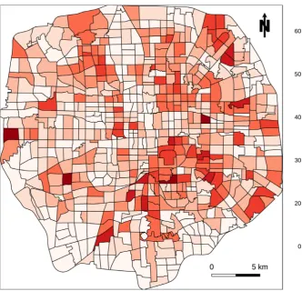
This study analyzed 686 TAZs within 668.55 km2 _{urban area of Beijing’s Fifth}

re-DOI: 10.4236/jdaip.2020.81001 6 Journal of Data Analysis and Information Processing search area, Figure 2 shows the frequency of different numbers of pedestrian crashes. The number of TAZs without any accidents is the most, accounting for 12.5%. With the number of pedestrian crashes increasing, the corresponding frequency is decreasing, meaning there are a few TAZs in unexpectedly higher

Figure 1. Pedestrian crash count per TAZ in Beijing.

DOI: 10.4236/jdaip.2020.81001 7 Journal of Data Analysis and Information Processing risk for pedestrians. The largest volume of accidents in one single TAZ reaches 65. The pedestrian crash number per TAZ varies a lot spatially, which will be analyzed in later sections.

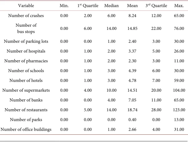
As mentioned above, many studies have combined accident data with tradi-tional traffic flow data and land use data to perform the spatial safety analysis. However, owing to the unavailability of these data at the TAZ level, we mainly focused on the POI data in this study. POI data are obtained from Google Ap-plication Programming Interface (API) through web scraping. After data tidying and categorizing, eleven kinds of POI were chosen, including bus stops, parking lots, hospitals, pharmacies, schools, hotels, supermarkets, banks, restaurants, parks and office buildings. Virtually, POI data are a special kind of land use data with concrete location attributes, which can be used to reflect the relationship between pedestrian crashes and user characteristics. Table 1 shows the statistical description of these POI data. Noticeably, mean values of crashes and POIs vary significantly, which indicates that the spatial distribution of data is exceptionally unbalanced at the spatial level.

4. Methodology

In this study, pedestrian crash data were analyzed from two aspects: spatial au-tocorrelation and spatial heterogeneity. According to Tobler’s first law of geo-graphy, near things are more correlated than distant things [40]. In other words, locations of traffic accidents are probably autocorrelated at the spatial level, es-pecially for different areas within a city. A group of spatial econometrics ap-proaches can be used to take the spatial autocorrelation into consideration, based on the traditional regression models. Spatial heterogeneity is the variation of relationship between variables due to variation of geographical positions. This

Table 1. POI data description at TAZ level.

Variable Min. 1st _{Quartile Median Mean 3}rd _{Quartile Max.}

Number of crashes 0.00 2.00 6.00 8.24 12.00 65.00

Number of

bus stops 0.00 6.00 14.00 14.85 22.00 76.00

Number of parking lots 0.00 0.00 1.00 2.40 3.00 30.00

Number of hospitals 0.00 1.00 2.00 3.37 5.00 26.00

Number of pharmacies 0.00 1.00 2.00 2.30 3.00 11.00

Number of schools 0.00 1.00 3.00 4.39 6.00 30.00

Number of hotels 0.00 1.00 3.00 4.78 7.00 59.00

Number of supermarkets 0.00 4.00 10.00 14.51 20.00 104.00

Number of banks 0.00 0.00 4.00 7.05 11.00 65.00

Number of restaurants 0.00 5.00 14.00 18.74 28.00 123.00

Number of parks 0.00 0.00 0.00 0.40 0.00 13.00

DOI: 10.4236/jdaip.2020.81001 8 Journal of Data Analysis and Information Processing issue can be solved by the Geographically Weighted Regression (GWR) [41].

4.1. Spatial Autoregression

In spatial analysis of traffic crashes, spatial dependence occurs when accidents of neighboring areas are correlated to each other. With this phenomenon existing, pedestrian crash data are not supposed to be directly analyzed by regular sion models, such as ordinary least squares (OLS). OLS is a type of linear regres-sion model for estimating unknown parameters, which can be expressed in a vector form as

y X=

β ε

(

)

~N 0, In

ε

σ

where y is the dependent variable of crash count, X represents explanatory

va-riables and β is a vector of coefficients of explanatory variables. ε is an error term, which is subject to normal distribution.

In a time-series context, the OLS estimator remains consistent even when a lagged dependent variable is present, as long as the error term does not show serial correlation. While the estimator may be biased in small samples, it can still be used for asymptotic inference. In a spatial context, this rule does not hold, ir-respective of the properties of the error term. In spatial analysis of traffic crashes, pure OLS can be used to find out the variables significant to the crash count of each TAZ, without considering any spatial relations of different areas. However, spatial autocorrelation in the crash data cannot be reflected just by the OLS. In order to deal with this issue, many transportation departments used OLS with a spatial weight matrix to model the number of crashes or the crash rate in a vast spatial scale over long time periods. To be more specific, several spatial econo-metrics approaches can be used for analyzing spatial autocorrelation in crash data on the basis of OLS results [42]. The spatial lag model (SLM) can be given by

y=ρWy X+ β ε+ (2)

(

)

~N 0, In

ε

σ

where y is the dependent variable, a vector (n × 1) of pedestrian crashes in one

year. W is a n × n spatial weight matrix, representing spatial relations between

spatial units. ρ is a spatial autoregressive coefficient. X is a n × k matrix of ex-planatory variables, and β is a k × 1 vector of parameters reflecting the impact of

explanatory variables on the y. ε is a n × 1 vector, defining unobserved error

terms that are independent and identically distributed.

Use of spatial error model (SEM) may be motivated by omitted variable bias. SEM is a regression model with spatial autocorrelation in the residuals defined by

y X= β µ+ (3)

W

DOI: 10.4236/jdaip.2020.81001 9 Journal of Data Analysis and Information Processing

(

)

~N 0, In

ε

σ

where y is the dependent variable, X represents explanatory variables, and β is a

vector of coefficients of X. W is a known spatial contiguity matrix. The

parame-ter λ is a coefficient on the autocorrelated residuals μ, and ε is an error term. The spatial Durbin model (SDM) adds spatial lag of both the dependent vari-able and explanatory varivari-ables into a traditional linear model, which can be ex-pressed by

1 2

y=ρWy X+ β +WXβ +ε ₍₅₎

(

)

~N 0, In

ε

σ

where y is a n × 1 vector of the dependent variable, X is the corresponding n × k

matrix which contains the observed explanatory variables, and β1 is a n × 1

vec-tor of associated parameters of X. W is a n × n spatial contiguity matrix, and ρ is

the coefficient of spatial lag of the dependent variable. The matrix product WX is

indicated for a spatial lag of the explanatory variables, and β2 is a k × 1 vector of

associated parameters.

In the SLM, the number of pedestrian crashes in a specific area is subject to spill-over effects from the number in adjacent regions. The spill-over effect can

be realized by spatial weight matrix W in the Equation (2). Similarly, the SEM

model assumes that the error in one region depends on the errors from

neigh-boring regions by W in the Equation (4). In this study, queen’s case [43] is used

to define the spatial weight matrix. The Queen’s case defines that regions sharing a common edge or common vertex are considered contiguous, and then the

corresponding element of the spatial weight matrix Wij is 1 but 0 otherwise. The

spdep package in R was used for this analysis.

4.2. Spatial Heterogeneity

A key assumption that we have made in the models thus far is that the structure of the model remains constant over the study area (no local variations in the pa-rameter estimates). However, spatial heterogeneity may exist across the spatial distribution of traffic crashes. Accounting for this, a GWR model mentioned before can be used to examine the potential spatial heterogeneity in parameter estimates. GWR permits the parameter estimates vary locally, similar to a para-meter drifts for time series model. GWR rewrites the linear model in a slightly different form, which can be expressed as

i i i

y =Xβ ε+ ₍₆₎

where i is the TAZ at which the local parameters are to be estimated. Here,

coef-ficient βi is allowed to be different between different TAZs. Parameters are

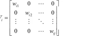
solved using a weighting scheme, which can be defined by

(

)

i X W Xi X W Yi

β = − ₍₇₎

DOI: 10.4236/jdaip.2020.81001 10 Journal of Data Analysis and Information Processing 1 2 0 0 0 0 0 0 i i i ij w w W w       =_{ }             

where the allocated weight wij for j observation at TAZ i is calculated with a

Gaussian function in this study, which can be expressed as 2 e ij d h ij w   −     

= ₍₉₎

where dijis the distance between the location of observation i and location j, and

the parameter h is the bandwidth.

It has been explained by a number of researchers that GWR model is affected more by the bandwidth than the kernel function [30] [31] [44]. The bandwidth is selected by minimization of root mean square error (RMSE). The GWR was established here using the spgwr package in R. Moran’s I was used to test if model’s residuals are spatially clustered [45]. Values of I range from −1 to 1 in general. If values are bigger than 0, they indicate positive spatial autocorrelation, while values below 0 indicate negative spatial autocorrelation. Exact 0 values of I indicate model’s residuals are randomly distributed. The Corrected Akaiki In-formation Criterion (AICc) was used to compare the performance of models [30] [31] [46]. The model of best fitting can be selected by the lowest AICc.

5. Results

5.1. Spatial Econometrics Analysis Results

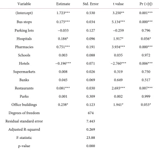
Firstly, an OLS model was established to examine points of interest whether they are significant to the number of pedestrian crashes in each TAZ. Results are shown in Table 2. Without considering spatial effects, pedestrian crash number of each TAZ is associated with the density of bus stops, hospitals, pharmacies, hotels, restaurants, office buildings, while parking lots, schools, supermarkets, banks, parks are not significant to crash count in the model.

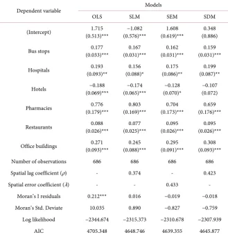
These POIs that do not pass the significance level in OLS were removed in the further analysis. The results of model performance of SLM, SEM and SDM are shown in the Table 3. The OLS was also re-established using six variables men-tioned before in order to compare with those models having considered the spa-tial autocorrelation. Almost all remained variables are statistically significant above 90% in four models. The coefficients of these variables are given in the Table 3, with their standard error in parenthesis. The number of observations is 686, which links to 686 TAZs including their data. The ρ coefficient is positive and highly significant in both SLM and SDM, indicating strong spatial

autocor-relation in the dependent variable. And the λ coefficient is positive and highly

DOI: 10.4236/jdaip.2020.81001 11 Journal of Data Analysis and Information Processing Table 2. Results for an OLS model based on all POI data.

Variable Estimate Std. Error t value Pr (>|t|)

(Intercept) 1.723*** 0.530 3.250** 0.001***

Bus stops 0.175*** 0.034 5.134*** 0.000***

Parking lots −0.033 0.127 −0.259 0.796

Hospitals 0.184* 0.096 1.917* 0.056*

Pharmacies 0.751*** 0.191 3.934*** 0.000***

Schools 0.003 0.088 0.035 0.972

Hotels −0.196*** 0.071 −2.760*** 0.006***

Supermarkets 0.008 0.026 0.319 0.750

Banks 0.045 0.069 0.649 0.517

Restaurants 0.081*** 0.030 2.693*** 0.007***

Parks 0.001 0.309 0.002 0.999

Office buildings 0.238* 0.123 1.941* 0.053*

Degrees of freedom 674

Residual standard error 7.443

Adjusted R-squared 0.269

F-statistic 23.88

p-value 0.000

*represents the significance level of 10%, **represents the significance level of 5%, and ***represents the significance level of 1%.

clustered in SLM, SEM and SDM respectively. Log likelihood and Akaiki infor-mation criterion (AIC) are chosen to compare the model performance. The low-er the log likelihood and AIC, the bettlow-er the model fit. From Table 3, three spa-tial regression models are better fit than OLS for both log likelihood and AIC. However, the performance of each spatial regression model is just close. Consi-dering only log likelihood, SDM results in a slightly better fit, while SEM results in the best fit for AIC evaluation.

DOI: 10.4236/jdaip.2020.81001 12 Journal of Data Analysis and Information Processing Table 3. Results for spatial models based on selected POI data.

Dependent variable Models

OLS SLM SEM SDM

(Intercept) _(0.513)*** 1.715 _(0.576)*** −1.082 _(0.619)*** 1.608 _(0.886) 0.348

Bus stops _(0.033)*** 0.177 _(0.031)*** 0.167 _(0.031)*** 0.162 _(0.031)*** 0.159

Hospitals _(0.093)** 0.193 _(0.088)* 0.156 _(0.086)** 0.175 _(0.087)** 0.199

Hotels _(0.069)*** −0.188 _(0.065)*** −0.174 _(0.070)* −0.128 −0.107 _(0.072)

Pharmacies _(0.179)*** 0.776 _(0.169)*** 0.803 _(0.173)*** 0.704 _(0.176)*** 0.659

Restaurants _(0.026)*** 0.088 _(0.025)*** 0.077 _(0.026)*** 0.095 _(0.026)*** 0.095

Office buildings _(0.093)*** 0.271 _(0.088)*** 0.245 _(0.091)*** 0.295 _(0.093)*** 0.308

Number of observations 686 686 686 686

Spatial lag coefficient (ρ) - 0.374 - 0.423

Spatial error coefficient (λ) - - 0.433 -

Moran’s I residuals 0.212*** 0.016 −0.019 −0.018

Moran’s Std. Deviate 10.035 0.890 −0.827 −0.759

Log likelihood −2344.674 −2315.373 −2310.678 −2307.939

AIC 4705.348 4648.746 4639.355 4645.877

Standard errors are in parenthesis. *represents the significance level of 10%, **represents the significance level of 5%, and ***represents the significance level of 1%.

DOI: 10.4236/jdaip.2020.81001 13 Journal of Data Analysis and Information Processing hotels can hardly be directly attractive for pure pedestrians, but can be for trav-elers using other kinds of traffic modes. Therefore, the chance of occurrence of pedestrian crashes would be relatively low.

5.2. Geographically Weighted Regression (GWR) Results

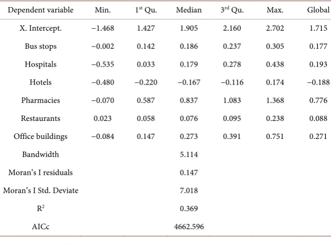
The results of the GWR model for pedestrian crashes are presented in Table 4. The bandwidth is 5.114, which was selected by the minimum value of RMSE

with a Gaussian kernel. The model’s R2 _{and corrected AIC are 0.369 and}

4662.596 respectively, indicating the model is well fitted. Because GWR esti-mates individual regression equations for all 686 TAZs, the minimum, first quarter, median, third quarter, maximum and global of the regression coeffi-cients for each independent variable are listed in the table.

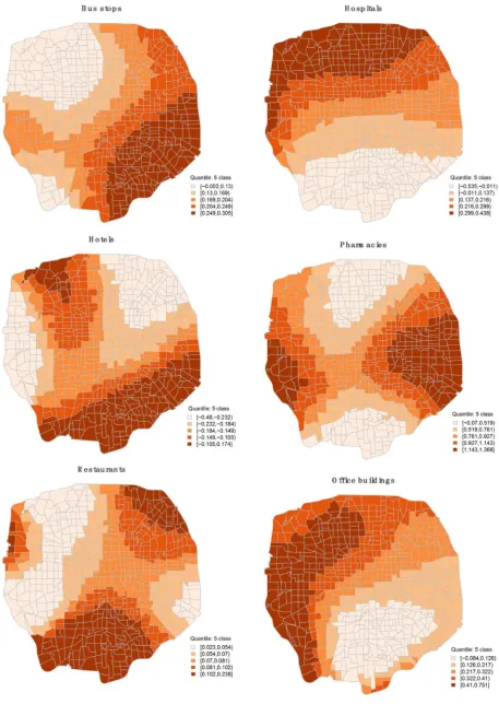
Based on the visualization of GWR results, it can be confirmed that different independent variables affect different regions within Beijing in obviously differ-ent ways. In order to improve pedestrian safety, suggestions ought to be pro-posed for those locations with risk higher than the average. Depending on six different POIs, the estimated coefficients for each TAZ are shown in the Figure 2. It is evident to see that different points of interest have different patterns of effect on each TAZ. For example, bus stops are more sensitive in south-eastern regions comparing to north-western regions. Pedestrians crashes occurring in northern regions are more affected by hospitals comparing to these in southern regions. What’s more, office buildings have stronger effect on both western and north-western regions than on other regions within fifth ring of Beijing. More susceptible are south-eastern and north-western regions for hotels, eastern and western regions for pharmacies and south and north-eastern regions for restau-rants.

Table 4. Results for GWR model based on selected POI data.

Dependent variable Min. 1st _{Qu. Median 3}rd _{Qu. Max. Global}

X. Intercept. −1.468 1.427 1.905 2.160 2.702 1.715

Bus stops −0.002 0.142 0.186 0.237 0.305 0.177

Hospitals −0.535 0.033 0.179 0.278 0.438 0.193

Hotels −0.480 −0.220 −0.167 −0.116 0.174 −0.188

Pharmacies −0.070 0.587 0.837 1.083 1.368 0.776

Restaurants 0.023 0.058 0.076 0.095 0.238 0.088

Office buildings −0.084 0.147 0.273 0.391 0.751 0.271

Bandwidth 5.114

Moran’s I residuals 0.147

Moran’s I Std. Deviate 7.018

R2 _0.369

DOI: 10.4236/jdaip.2020.81001 14 Journal of Data Analysis and Information Processing Considering the different effects of independent variables on the each TAZ, some localized strategies could be proposed to improve the traffic safety for pe-destrians. For instance, TAZs in the northeast of Beijing should make a safer en-vironment of pedestrians taking buses. Northern areas may need more traffic management around hospitals to better protect pedestrians. These recommen-dations require many practical experiences and need to be adjusted, and they are worthy of taking into account in urban management plans.

6. Conclusions

This study mainly used several spatial regression models to estimate the correla-tion between various points of interest and pedestrian crashes. Firstly, a tradi-tional OLS model was built to remove those independent variables not statisti-cally significant to the pedestrian crash count for each TAZ. Then three spatial models, SLM, SEM and SDM, were established to examine if the spatial autocor-relation exists in the pedestrian crash data comparing to the OLS model. Ac-cording to values of AICc, SEM model outperformed other two spatial models as well as the OLS model. Additionally, a GWR model with Gussian kernel was de-veloped to examine the spatial heterogeneity of different explanatory variables on different locations within Beijing urban area. Visualization of GWR results helped us better understand the effect of different POIs on each TAZ (see Figure 3).

Eleven kinds of POI were tested in OLS, while only six of them were signifi-cant to the pedestrian crash count of TAZs, including bus stops, hospitals, ho-tels, pharmacies, restaurants, and office buildings. All these POIs were proven to have a positive correlation with the number of pedestrian crashes for each TAZ except hotels. With spatial dependence into consideration, the results of spatial model SLM, SEM and SDM demonstrated that these six POIs are still credibly correlated with the occurrence of pedestrian crashes, while only the significance level varies a little. The GWR model revealed that the effect of different POIs on each TAZ is generally different. For example, the occurrence of pedestrian crashes in northern urban areas of Beijing is more subject to hospitals than in the south, while bus stops have a stronger effect on the south-eastern regions than the north-western regions.

DOI: 10.4236/jdaip.2020.81001 16 Journal of Data Analysis and Information Processing practical implementations and advanced computer technologies in order to bet-ter integrate traffic safety analysis into planning and ultimately realize a safer city for all our citizens. It is recommended that further study will be able to identify the optimum spatial scale for analyzing the characteristics of pedestrian crashes and proposing more meaningful improvements.

Acknowledgements

This study was sponsored by the National Key R&D Program of China (2017YFC0803903).

Conflicts of Interest

The authors declare no conflicts of interest regarding the publication of this pa-per.

References

[1] World Health Organization (2018) Global Status Report on Road Safety.

https://www.who.int/violence_injury_prevention/road_safety_status/2018/en

[2] Kamruzzaman, M., Haque, M.M. and Washington, S. (2014) Analysis of Traffic Injury Severity in Dhaka, Bangladesh. Transportation Research Record, 2451, 121-130. https://doi.org/10.3141/2451-14

[3] Lee, J., Abdel-Aty, M. and Jiang, X. (2015) Multivariate Crash Modeling for Motor Vehicle and Non-Motorized Modes at the Macroscopic Level. Accident Analysis and Prevention, 78, 146-154.https://doi.org/10.1016/j.aap.2015.03.003

[4] Ding, C., Chen, P. and Jiao, J. (2018) Non-Linear Effects of the Built Environment on Automobile-Involved Pedestrian Crash Frequency: A Machine Learning Ap-proach. Accident Analysis and Prevention, 112, 116-126.

https://doi.org/10.1016/j.aap.2017.12.026

[5] Lee, J., Abdel-Aty, M. and Shah, I. (2018) Evaluation of Surrogate Measures for Pe-destrian Trips at Intersections and Crash Modeling. Accident Analysis and Preven-tion, 130, 91-98.https://doi.org/10.1016/j.aap.2018.05.015

[6] Hannah, C., Spasić, I. and Corcoran, P. (2018) A Computational Model of Pede-strian Road Safety: The Long Way Round Is the Safe Way Home. Accident Analysis and Prevention, 121, 347-357.https://doi.org/10.1016/j.aap.2018.06.004

[7] Pour-Rouholamin, M. and Zhou, H. (2016) Investigating the Risk Factors Asso-ciated with Pedestrian Injury Severity in Illinois. Journal of Safety Research, 57, 9-17.https://doi.org/10.1016/j.jsr.2016.03.004

[8] Ma, Z., Lu, X., Chien, S.I. and Hu, D. (2017) Investigating Factors Influencing Pe-destrian Injury Severity at Intersections. Traffic Injury Prevention, 19, 159-164. https://doi.org/10.1080/15389588.2017.1354371

[9] Kim, M., Kho, S. and Kim, D. (2017) Hierarchical Ordered Model for Injury Severi-ty of Pedestrian Crashes in South Korea. Journal of Safety Research, 61, 33-40. https://doi.org/10.1016/j.jsr.2017.02.011

[10] Xie, X., Nikitas, A. and Liu, H. (2018) A Study of Fatal Pedestrian Crashes at Rural Low-Volume Road Intersections in Southwest China. Traffic Injury Prevention, 19, 298-304.https://doi.org/10.1080/15389588.2017.1387654

DOI: 10.4236/jdaip.2020.81001 17 Journal of Data Analysis and Information Processing

Severity by Party at Fault in San Francisco, CA. Accident Analysis and Prevention, 110, 149-160.https://doi.org/10.1016/j.aap.2017.11.007

[12] Siddiqui, C., Abdel-Aty, M. and Choi, K. (2012) Macroscopic Spatial Analysis of Pedestrian and Bi-Cycle Crashes. Accident Analysis and Prevention, 45, 382-391. https://doi.org/10.1016/j.aap.2011.08.003

[13] Wang, Y. and Kockelman, K.M. (2013) A Poisson-Lognormal Condition-al-Autoregressive Model for Multivariate Spatial Analysis of Pedestrian Crash Counts across Neighborhoods. Accident Analysis and Prevention, 60, 71-84. https://doi.org/10.1016/j.aap.2013.07.030

[14] Amoh-Gyimah, R., Saberi, M. and Sarvi, M. (2016) Macroscopic Modeling of Pede-strian and Bicycle Crashes: Across-Comparison of Estimation Methods. Accident Analysis and Prevention, 93, 147-159.

https://doi.org/10.1016/j.aap.2016.05.001

[15] Cai, Q., Lee, J., Eluru, N. and Abdel-Aty, M. (2016) Macro-Level Pedestrian and Bi-cycle Crash Analysis: Incorporating Spatial Spillover Effects in Dual State Count Models. Accident Analysis and Prevention, 93, 14-22.

https://doi.org/10.1016/j.aap.2016.04.018

[16] Wang, X., Yang, J., Lee, C., Ji, Z. and You, S. (2016) Macro-Level Safety Analysis of Pedestrian Crashes in Shanghai, China. Accident Analysis and Prevention, 96, 12-21.https://doi.org/10.1016/j.aap.2016.07.028

[17] Medury, A. and Grembek, O. (2016) Dynamic Programming-Based Hot Spot Iden-tification Approach for Pedestrian Crashes. Accident Analysis and Prevention, 93, 198-206.https://doi.org/10.1016/j.aap.2016.04.037

[18] Erdogan, S., Yilmaz, I., Baybura, T. and Gullu, M. (2008) Geographical Information Systems Aided Traffic Accident Analysis System Case Study: City of Afyonkarahi-sar. Accident Analysis and Prevention, 40, 174-181.

https://doi.org/10.1016/j.aap.2007.05.004

[19] Bíl, M., Andrášik, R. and Janoška, Z. (2013) Identification of Hazardous Road Loca-tions of Traffic Accidents by Means of Kernel Density Estimation and Cluster Signi-ficance Evaluation. Accident Analysis and Prevention, 55, 265-273.

https://doi.org/10.1016/j.aap.2013.03.003

[20] Hashimoto, S., Yoshiki, S., Saeki, R., Mimura, Y., Ando, R. and Nanba, S. (2016) Development and Application of Traffic Accident Density Estimation Models Using Kernel Density Estimation. Journal of Traffic and Transportation Engineering, 3, 262-270.https://doi.org/10.1016/j.jtte.2016.01.005

[21] Xie, Z. and Yan, J. (2008) Kernel Density Estimation of Traffic Accidents in a Net-work Space. Computers, Environment and Urban Systems, 32, 396-406.

https://doi.org/10.1016/j.compenvurbsys.2008.05.001

[22] Mohaymany, A.S., Shahri, M. and Mirbagheri, B. (2013) GIS-Based Method for De-tecting High-Crash-Risk Road Segments Using Network Kernel Density Estimation. Geo-Spatial Information Science, 16, 113-119.

https://doi.org/10.1080/10095020.2013.766396

[23] Harirforoush, H. and Bellalite, L. (2016) A New Integrated GIS-Based Analysis to Detect Hotspots: A Case Study of the City of Sherbrooke. Accident Analysis and Prevention, 130, 62-74.https://doi.org/10.1016/j.aap.2016.08.015

[24] Pulugurtha, S.S., Krishnakumar, V.K. and Nambisan, S.S. (2007) New Methods to Identify and Rank High Pedestrian Crash Zones: An Illustration. Accident Analysis and Prevention, 39, 800-811.https://doi.org/10.1016/j.aap.2006.12.001

Pe-DOI: 10.4236/jdaip.2020.81001 18 Journal of Data Analysis and Information Processing

destrian Crashes in Santiago, Chile. Accident Analysis and Prevention, 50, 304-311. https://doi.org/10.1016/j.aap.2012.05.001

[26] Nicholson, A. (1999) Analysis of Spatial Distributions of Accidents. Safety Science, 31, 71-91.https://doi.org/10.1016/S0925-7535(98)00056-3

[27] Xie, K., Ozbay, K. and Yang, H. (2019) A Multivariate Spatial Approach to Model Crash Counts by Injury Severity. Accident Analysis and Prevention, 122, 189-198. https://doi.org/10.1016/j.aap.2018.10.009

[28] Saha, D., Alluri, P., Gan, A. and Wu, W. (2018) Spatial Analysis of Macro-Level Bi-cycle Crashes Using the Class of Conditional Autoregressive Models. Accident Analysis and Prevention, 118, 166-177.https://doi.org/10.1016/j.aap.2018.02.014

[29] Jia, R., Khadka, A. and Kim, I. (2018) Traffic Crash Analysis with Point-of-Interest Spatial Clustering. Accident Analysis and Prevention, 121, 223-230.

https://doi.org/10.1016/j.aap.2018.09.018

[30] Bao, J., Liu, P., Yu, H. and Xu, C. (2017) Incorporating Twitter-Based Human Ac-tivity Information in Spatial Analysis of Crashes in Urban Areas. Accident Analysis and Prevention, 106, 358-369.https://doi.org/10.1016/j.aap.2017.06.012

[31] Rhee, K., Kim, J., Lee, Y. and Ulfarsson, G.F. (2016) Spatial Regression Analysis of Traffic Crashes in Seoul. Accident Analysis and Prevention, 91, 190-199.

https://doi.org/10.1016/j.aap.2016.02.023

[32] Blazquez, C.A., Picarte, B., Calderón, J.F. and Losada, F. (2018) Spatial Autocorrela-tion Analysis of Cargo Trucks on Highway Crashes in Chile. Accident Analysis and Prevention, 120, 195-210.https://doi.org/10.1016/j.aap.2018.08.022

[33] Simões, P. (2015) A Spatial Econometrics Analysis for Road Accidents in Lisbon. International Journal of Business Intelligence and Data Mining, 10, 152-173. https://doi.org/10.1504/IJBIDM.2015.069270

[34] Kaplan, S. and Prato, C.G. (2015) A Spatial Analysis of Land Use and Network Ef-fects on Frequency and Severity of Cyclist-Motorist Crashes in the Copenhagen Re-gion. Traffic Injury Prevention, 16, 724-731.

https://doi.org/10.1080/15389588.2014.1003818

[35] Wang, X., Zhou, Q., Yang, J., You, S., Song, Y. and Xue, M. (2019) Macro-Level Traffic Safety Analysis in Shanghai, China. Accident Analysis and Prevention, 125, 249-256.https://doi.org/10.1016/j.aap.2019.02.014

[36] Xu, P. and Huang, H. (2015) Modeling Crash Spatial Heterogeneity: Random Para-meter versus Geographically Weighting. Accident Analysis and Prevention, 75, 16-25. https://doi.org/10.1016/j.aap.2014.10.020

[37] Gomes, M.J.T.L., Cunto, F. and Silva, A.R. (2017) Geographically Weighted Nega-tive Binomial Regression Applied to Zonal Level Safety Performance Models. Acci-dent Analysis and Prevention, 106, 254-261.

https://doi.org/10.1016/j.aap.2017.06.011

[38] Cai, Q., Lee, J., Eluru, N. and Abdel-Aty, M. (2016) Macro-Level Pedestrian and Bi-cycle Crash Analysis: Incorporating Spatial Spillover Effects in Dual State Count Models. Accident Analysis and Prevention, 93, 14-22.

https://doi.org/10.1016/j.aap.2016.04.018

[39] Guo, Q., Xu, P., Pei, X., Wong, S.C. and Yao, D. (2017) The Effect of Road Network Patterns on Pedestrian Safety: A Zone-Based Bayesian Spatial Modeling Approach. Accident Analysis and Prevention, 99, 114-124.

https://doi.org/10.1016/j.aap.2016.11.002

DOI: 10.4236/jdaip.2020.81001 19 Journal of Data Analysis and Information Processing

Region. Economic Geography, 46, 234-240.https://doi.org/10.2307/143141

[41] Fotheringham, A.S., Brundson, C. and Charlton, M.E. (2002) Geographically Weighted Regression: The Analysis of Spatially Varying Relationships. John Wiley and Sons Ltd., West Sussex.

[42] Simões, P. and Natário, I. (2016) Spatial Econometric Approaches for Count Data: An Overview and New Directions. International Journal of Economics and Man-agement Engineering, 10, 348-357.

[43] Anselin, L. and Griffith, D.A. (1988) Do Spatial Effects Really Matter in Regression Analysis? The Regional Science Association International, 65, 11-34.

https://doi.org/10.1111/j.1435-5597.1988.tb01155.x

[44] Erdogan, S. (2009) Explorative Spatial Analysis of Traffic Accident Statistics and Road Mortality among the Provinces of Turkey. Journal of Safety Research, 40, 341-351.https://doi.org/10.1016/j.jsr.2009.07.006

[45] Moran, P.A.P. (1950) Notes on Continuous Stochastic Phenomena. Biometrika, 37, 17-23.https://doi.org/10.1093/biomet/37.1-2.17