Multilayer Sequence Labeling
Ai Azuma Yuji Matsumoto
Graduate School of Information Science Nara Institute of Science and Technology
Ikoma, Nara 630-0192, Japan
{ai-a,matsu}@is.naist.jp
Abstract
In this paper, we describe a novel approach to cascaded learning and inference on sequences. We propose a weakly joint learning model on cascaded inference on sequences, called multilayer sequence labeling. In this model, inference on sequences is modeled as cas-caded decision. However, the decision on a sequence labeling sequel to other decisions utilizes the features on the preceding results as marginalized by the probabilistic models on them. It is not novel itself, but our idea central to this paper is that the probabilis-tic models on succeeding labeling are viewed as indirectly depending on the probabilistic models on preceding analyses. We also pro-pose two types of efficient dynamic program-ming which are required in the gradient-based optimization of an objective function. One of the dynamic programming algorithms re-sembles back propagation algorithm for mul-tilayer feed-forward neural networks. The other is a generalized version of the forward-backward algorithm. We also report experi-ments of cascaded part-of-speech tagging and chunking of English sentences and show ef-fectiveness of the proposed method.
1 Introduction
Machine learning approach is widely used to clas-sify instances into discrete categories. In many tasks, however, some set of inter-related labels should be decided simultaneously. Such tasks are called structured prediction. Sequence labeling is the simplest subclass of structured prediction prob-lems. In sequence labeling, the most likely one
among all the possible label sequences is predicted for a given input. Although sequence labeling is the simplest subclass, a lot of real-world tasks are modeled as problems of this simplest subclass. In addition, it might offer valuable insight and a toe-hold for more general and complex structured pre-diction problems. Many models have been proposed for sequence labeling tasks, such as Hidden Markov Models (HMM), Conditional Random Fields (CRF) (Lafferty et al., 2001), Max-Margin Markov Net-works (Taskar et al., 2003) and others. These models have been applied to lots of practical tasks in natural language processing (NLP), bioinformatics, speech recognition, and so on. And they have shown great success in recent years.
In real-world tasks, it is often needed to cascade multiple predictions. A cascade of predictions here means the situation in which some of predictions are made based upon the results of other predictions. Sequence labeling is not an exception. For exam-ple, in NLP, we perform named entity recognition or base-phrase chunking for given sentences based on part-of-speech (POS) labels predicted by another se-quence labeler. Natural languages are especially in-terpreted to have a hierarchy of sequential structures on different levels of abstraction. Therefore, many tasks in NLP are modeled as a cascade of sequence predictions.
If a prediction is based upon the result of another prediction, we call the former upper stage and the latter lower stage.
Methods pursued for a cascade of predictions – including sequence predictions, of course–, are sired to perform certain types of capability. One
sired capability is rich forward information propa-gation, that is, the learning and estimation on each stage of predictions should utilize rich informa-tion of the results of lower stages whenever pos-sible. “Rich information” here includes next bests and confidence information of the results of lower stages. Another is backward information propaga-tion, that is, the rich annotated data on an upper stage should affect the models on lower stages retroac-tively.
Many current systems for a cascade of sequence predictions adopt a simple1-best feed-forward ap-proach. They simply take the most likely output at each prediction stage and transfer it to the next upper stage. Such a framework can maximize reusability of existing sequence labeling systems. On the other hand, it exhibits a strong tendency to propagate er-rors to upper labelers.
Typical improvement on the 1-best approach is to keepk-best results in the cascade of predictions. However, the largerkbecomes, the more difficult it is to enumerate and maintain thek-best results. It is particularly prominent in sequence labeling.
The essence of this orientation is that the labeler on an upper stage utilizes the information of all the possible output candidates on lower stages. How-ever, the size of the output space can become quite large in sequence labeling. It effectively forbids ex-plicit enumeration of all possible outputs, so it is required to represent all the labeling possibilities compactly or employ some approximation schemes. Several studies are in this direction. In the method proposed in Finkel et al. (2006), a cascades of se-quence predictions is viewed as a Bayesian network, and sample sequences are drawn at each stage ac-cording to the output distribution. The samples are then used to estimate the entire distribution of the cascade. In the method proposed in Bunescu (2008), an upper labeler uses the probabilities marginalized on the parts of the output sequences on lower stages as weights for the features. The weighted features are integrated in the model of the labeler on the upper stage. Ak-best approach (e.g., (Collins and Duffy, 2002)) and the methods mentioned above are effective to improve the forward information propa-gation. However, they can never contribute on back-ward information propagation.
To improve the both directions of information
propagation, Some studies propose the joint learning of multiple sequence labelers. Sutton et al. (2007) proposes the joint learning method in case where multiple labels are assigned to each time slice of the input sequences. It enables simultaneous learn-ing and estimation of multiple sequence labellearn-ings on the same input sequences, where time slices of the outputs of all the out sequences are regularly aligned. However, it puts the distribution of states into Bayesian networks with cyclic dependencies, and exact inference is not tractable in such a model in general. Therefore, it requires some approxi-mate inference algorithms in learning or predictions. Moreover, it only considers the cases where labels of an input sequence and all output sequences are reg-ularly aligned. It is not clear how to build a joint labeling model which handles irregular output label sequences like semi-Markov models (Sarawagi and Cohen, 2005).
In this paper, we propose a middle ground for a cascade of sequence predictions. The proposed method adopts the basic idea of Bunescu (2008). We first assume that the model on all the sequence la-beling stages is probabilistic one. In modeling of an upper stage, a feature is weighted by the marginal probability of the fragment of the outputs from a lower stage. However, this is not novel itself be-cause it is just a paraphrase of Bunescu’s core idea. Our intuition behind the proposed method is as fol-lows. Features integrated in the model on each stage are weighted by the marginal probabilities of the fragments of the outputs on lower stages. So, if the output distributions on lower stages change, the marginal probabilities of any fragments also change, and this in turn can change the value of the features on the upper stage. In other words, the features on an upper stage indirectly depend on the models on the lower stages. Based on this intuition, the learn-ing procedure of the model on an upper stage can affect not only direct model parameters, but also the weights of the features by changing the model on the lower stages. Supervised learning based on an-notated data on an upper stage may affect the model or model parameters on the lower stages. It could be said that the information of annotation data on an upper stage is propagated back to the model on lower stages.
nota-tion of our model. In Secnota-tion 3, we propose an opti-mization procedure according to the intuition noted above. In Section 4, we report an experimental result of our method. The proposed method shows some improvements on a real-world task in comparison with ordinary methods.
2 Formalization
In this section, we introduce the formal notation of our model. Hereafter, for the sake of simplicity, we only describe the simplest case in which there are just two stages, one lower stage of sequence labeling namedL1and one upper stage of sequence labeling namedL2. InL1,the most likely one among a set of possible sequences is predicted for a given input x.L2is also a sequence labeling stage for the same inputxand the output ofL1. No assumption is made on the structure ofx. The information ofxis totally encoded in feature functions. It is only assumed that the output spaces of bothL1andL2are conditioned on the initial inputx.
First of all, we describe the formalization of the probabilistic model forL1. The model for L1 per se is the same as ordinary ones for sequence label-ing. For a given inputx,consider a directed acyclic graph (DAG)G1 = (V1, E1). A source of a DAGG is a node whose in-degree is equal to zero. A sink of a DAGGis nodes whose out-degree is equal to zero. Let src(G), snk(G) denote the set of source and sink nodes inG, respectively. A successful path of a DAGGis defined as a directed path onGwhose starting node is a source and end node is a sink. Ify denotes a path on a DAG, letyalso denote the set of all the arcs appearing onyfor the sake of shorthand. We denote the set of all the possible successful paths onG1byY1. The space of the output candidates for
L1is exactly equal toY1. For the modeling ofL1, it is assumed that features of the formf⟨1,k1,e1,x⟩∈R
(k1∈ K1, e1 ∈E1) are allowed to be used. Here, K1 is the index set of the feature types forL1. Such a feature can capture an aspect of the correlation be-tween adjacent nodes. We call this kind of features input features forL1. This naming is used to distin-guish them from another kind of features defined on
L1, which comes later. Although features onV1can be also defined, they are totally omitted in this paper for brevity. Hereafter, if a symbol has subscripts,
then missing subscript indicates a set that range over the omitted subscript. For example, f⟨1,e1,x⟩ def≡
{
f⟨1,k1,e1,x⟩}k
1∈K1,f⟨1,k1,x⟩ def
≡ {f⟨1,k1,e1,x⟩}e
1∈E1, f⟨1,x⟩ def≡ {f⟨1,k1,e1,x⟩}
k1∈K1,e1∈E1, and so on. The probabilistic model onL1 forms the log-linear model, that is,
P1(y1|x;θ1) def
≡ Z 1 1(x;θ1)
exp(θ1·F⟨1,y1,x⟩
)
(y1 ∈Y1) , (1) whereθ⟨1,k1⟩ ∈ R (k1∈ K1)is the weight for the feature of the same indexk1, and thek1-th element ofF⟨1,y1,x⟩, F⟨1,k1,y1,x⟩def≡ ∑e1∈y1f⟨1,k1,e1,x⟩. Dot operator (·) denotes the inner product with respect to the subscripts commonly missing in both operands.
Z1is the partition function forP1, defined as
Z1(x;θ1) def
≡ ∑
y1∈Y1
exp(θ1·F⟨1,y1,x⟩
)
. (2)
It is worth noting that this formalization subsumes both directed and undirected linear-chain graphical models, which are the most typical models for se-quence labeling, including HMM and CRF. That is, if the elements of V1 are aligned into regular time slices, and the nodes in each time slice are associated with possible assignments of labels for that time, we obtain the representation equivalent to the ordinary linear-chain graphical models, in which all possible label assignments for each state are expanded. In such configuration, all the possible successful paths defined in our notation have strict one-to-one corre-spondence to all the possible joint assignments of labels in linear-chain graphical models. We pur-posely employ this DAG-based notation because; it is convenient to describe the models and algorithms for our purpose, it allows for labels to stay in arbi-trary time as in semi-Markov models, and it is easily extended to models for a set of trees instead of se-quences by replacing the graph-based notation with hypergraph-based notation.
The form of the features available in designing the probabilistic model forL2, denoted byP2, is the key of this paper. A feature on an arce2 ∈ E2 can ac-cess local characteristics of the confidence-rated su-perposition of the L1’s outputs, in addition to the information of the inputx. To formulate local char-acteristics of the superposition of theL1’s outputs, we first define output features of L1, denoted by
h⟨1,k′
1,e1⟩ ∈ R (k1′ ∈ K′1, e1∈E1). Here, K′1 is the index set of the output feature types ofL1. Be-fore the output features are integrated into the model forL2, they all are confidence-rated with respect to
P1, that is, each output feature h⟨1,k′
1,e1⟩ is numer-ically rated by the estimated probabilities summed over the sequences emitting that feature. More for-mally, all theL1’s output features are integrated in features forP2 in the form of the marginalized out-put features, which are defined as follows;
¯
h⟨1,k′
1,e1⟩(θ1) def
≡ h⟨1,k′
1,e1⟩P1(e1|x;θ1)
(
k′1∈ K′1, e1 ∈E1) , (3)
where
P1(e1|x;θ1) def
≡ ∑
y1∼e1
P1(y1|x;θ1)
= ∑
y1∈Y1
δe1∈y1P1(y1|x;θ1)
(e1 ∈E1) . (4)
Here, the notation ∑y1∼e1 represents the sum-mation over sequences consistent with an arc
e1 ∈ E1, that is, the summation over the set {y1 ∈Y1 |e1∈y1}. δP denotes the indicator
function for a predicateP. The input features forP2 on an arce2 ∈ E2 are permitted to arbitrarily com-bine the information ofxand theL1’s marginalized output features h¯1, in addition to the local charac-teristics of the arc at hande2. In summary, an input feature forL2on an arce2 ∈E2is of the form
f⟨2,k2,e2,x⟩(h¯1(θ1)
)
∈R (k2 ∈ K2) , (5)
whereK2 is the index set of the input feature types forL2. To make the optimization procedure feasible, smoothness condition on any L2’s input feature is assumed with respect to all theL1’s output features, that is, ∂f⟨2,k2,e2,x⟩
∂¯h⟨1,k′
1,e1⟩
is always guaranteed to exist for
∀k′
1, e1, k2, e2. For example, additions and mul-tiplications between some elements of h¯1(θ1) can appear in the definition ofL2’s input features. For given input featuresf⟨2,x⟩
(¯
h1(θ1)) and parameters
θ⟨2,k2⟩ ∈ R (k2 ∈ K2), the probabilistic model for
L2is defined as follows;
P2(y2|x;θ1,θ2)
def
≡ Z 1 2(x;θ1,θ2)
exp(θ2·F⟨2,y2,x⟩
(¯
h1(θ1)
))
(y2 ∈Y2) , (6) where F⟨2,k2,y2,x⟩
(¯
h1(θ1))
def ≡
∑
e2∈y2f⟨2,k2,e2,x⟩
(¯
h1(θ1)
)
and Z2 is the par-tition function ofP2, defined by
Z2(x;θ1,θ2) def
≡ ∑
y2∈Y2
exp(θ2·F⟨2,y2,x⟩
(¯
h1(θ1))) .
(7) The definition ofP2 (6) reveals one of the most im-portant points in this paper. P2 is viewed not only as the function of the ordinary direct parametersθ2 but also as the function ofθ1, which represents the parameters for theL1’s model, through the interme-diate variablesh¯1. So optimization procedure onP2 may affect the determination of the values not only of the direct parameters θ2 but also of the indirect onesθ1.
If the result ofL1 is reduced to the single golden outputy˜1, i.e. P1(y1|x) = δy1=˜y1, the definitions above boil down to the formulation of the simple 1-best feed forward architecture.
3 Optimization Algorithm
In this section, we describe optimization procedure for the model formulated in the previous section. LetD ={⟨xˆ,⟨G1,yˆ1⟩,⟨G2,yˆ2⟩⟩m}m=1,2,···,M de-note annotated data for the supervised learning of the model. Here,⟨G1,yˆ1⟩ is a pair of a DAG and correctly annotated successful sequence forL1. The same holds for⟨G2,yˆ2⟩. For givenD, we can define the conditional log-likelihood function onL1andL2 respectively, that is,
L1(θ1;D) def
≡ ∑
⟨xˆ,ˆy1⟩∈D
log (P1(ˆy1|x;ˆ θ1))− | θ1| 2σ12
Figure 1: Computation Graph of the Proposed Model
and
L2(θ1,θ2;D) def
≡ ∑
⟨xˆ,ˆy2⟩∈D
log (P2(ˆy2|x;ˆ θ1,θ2))− | θ2| 2σ22
.
(9) Here,σ12,σ22are the variances of the prior distribu-tions of the parameters. For the sake of simplicity, we set the prior distribution as the zero-mean uni-variance Gaussian. To optimize the both probabilis-tic modelsP1andP2jointly, we also define the joint conditional log-likelihood function
L(θ1,θ2;D) def
≡ L1+L2 . (10)
The parameter values to be learned are the ones that (possibly locally) maximize this objective function. Note that this objective function is not guaranteed to be globally convex.
We employ gradient-based parameter optimiza-tion here. Optimization procedure repeatedly searches a direction in the parameter space which is ascendent with respect to the objective function, and updates the parameter values into that direction by small advances. Many existing optimization rou-tines like steepest descent or conjugation gradient do that job only by giving the objective value and gra-dients on parameter values to be updated. So, the optimization problem here boils down to the calcu-lation of the objective value and gradients on given parameter values.
Before entering the detailed description of the al-gorithm for calculating the objective function and gradients, we note the functional relations among the objective function and previously defined vari-ables. The diagram shown in Figure 1 illustrates the functional relations among the parameters, input and output feature functions, models, and objective function. The variables at the head of a directed ar-row in the figure is directly defined in terms of the ones at the tail of the same arrow. The value of the
objective function on given parameter values can be calculated in order of the arrows shown in the di-agram. On the other hand, the parameter gradients are calculated step-by-step in reverse order of the ar-rows. The functional relations illustrated in the Fig-ure 1 ensFig-ure some forms of the chain rule of dif-ferentiation among the variables. The chain rule is iteratively used to decompose the calculation of the gradients into a divide-and-conquer fashion. These two directions of stepwise computation are analo-gous to the forward and back propagation for multi-layer feedforward neural networks, respectively.
Algorithm 1 shows the whole picture of the gradient-based optimization procedure for our model. We first describe the flow to calculate the objective value for a given parameters θ1 and θ2, which is shown from line 2 through 4 in Algo-rithm 1. The values of marginalized output features ¯
h⟨1,x⟩can be calculated by (3). Because they are the simple marginals of features, the ordinary forward-backward algorithm (hereafter, abbreviated as “F-B”) onG1 offers an efficient way to calculate their values. Although nothing definite about the forms of the input features forL2 is presented in this pa-per,f⟨2,x⟩can be calculated once the values ofh¯⟨1,x⟩ have been obtained. Finally,L1,L2and thenLare easy to calculate because they are no different from the ordinary log-likelihood computation.
Now we describe the algorithm to calculate the parameter gradients,
∂L ∂θ1
= ∂L1
∂θ1
+∂L2
∂θ1
, ∂L
∂θ2
= ∂L2
∂θ2
. (11)
Line 5 through line 7 in Algorithm 1 describe the gradient computation. The terms ∂L1
∂θ1 and ∂L2 ∂θ2 in (11) become the same forms that appear in the ordi-nary CRF optimization, i.e., the difference between the empirical frequencies of the features and the model expectations of them,
∂L1
∂θ1
= ˜E[F⟨1,y1,x⟩
]
−EP1
[
F⟨1,y1,x⟩
]
−|θ1|
σ12
,
∂L2
∂θ2
= ˜E[F⟨2,y2,x⟩
]
−EP2
[
F⟨2,y2,x⟩
]
−|θ2|
σ22
.
(12) These calculations are performed by the ordinary F-B onG1 andG2, respectively. Using the chain rule of differentiation derived from the functional rela-tions illustrated in Figure 1, the remaining term ∂L2
Algorithm 1 Gradient-based optimization of the model parameters Input: θ1,θ2
Output: arg max
⟨θ1,θ2⟩ L
1: whileθ1orθ2changes significantly do
2: calculateZ1 by (2),h¯1by (3) with the F-B onG1, and thenL1by (8)
3: calculatef⟨2,x⟩according to their definitions
4: calculateZ2 by (7) with the F-B onG2, and thenL2by (9) andLby (10)
5: calculate ∂L1 ∂θ1 and
∂L2
∂θ2 by (12) with the F-B onG1andG2, respectively
6: calculate ∂f∂L
⟨1,x⟩ by (16) with the F-B onG2,
∂f⟨1,x⟩
∂h¯1 , and them ∂L2 ∂h¯1 =
∂L
∂f⟨1,x⟩ ·
∂f⟨1,x⟩
∂h¯1
7: calculate ∂L2
∂θ1 by (18) with Algorithm 2
8: ⟨θ1,θ2⟩ ←update-parameters
(
θ1,θ2,L,∂∂θL1, ∂L
∂θ2
)
9: end while
in (11) can be decomposed as follows;
∂L2
∂θ1
= ∂L2
∂f⟨2,x⟩ ·
∂f⟨2,x⟩
∂θ1
= ∂L2
∂f⟨2,x⟩ ·
∂f⟨2,x⟩
∂h¯1 ·
∂h¯1
∂θ1
.
(13) Note that Leibniz’s notation here denotes a Jacobian with the index sets omitted in the numerator and the denominator, for example,
∂f⟨2,x⟩
∂h¯1 def
≡
{
∂f⟨2,k2,e2,x⟩ ∂h⟨1,k′
1,e1⟩
}
k2∈K2,e2∈E2,k′1∈K′1,e1∈E1 (14) And also recall that dot operators here stand for the inner product with respect to the index sets com-monly omitted in both operands, for example,
∂L2
∂f2 ·
∂f2
∂h¯1
= ∑
k2∈K2,e2∈E2
∂L2
∂f⟨2,k2,e2,x⟩ ·
∂f⟨2,k2,e2,x⟩ ∂h¯1
.
(15) We describe the manipulation of each factor in the right side of (13) in turn. Noting ∂f⟨2,k2,e2,x⟩
∂f⟨2,`k2,`e2,x⟩ =
δk
2=`k2δe2=`e2, each element of the first factor of (13) ∂L2
∂f⟨2,x⟩ can be transformed as follows;
∂L2
∂f⟨2,k2,e2,x⟩
=θ⟨2,k2⟩ ∑ ⟨xˆ,ˆy2⟩∈D
(
δe2∈yˆ2 −P2(e2|x;ˆ θ1,θ2)
)
.
(16)
P2(e2|x;ˆ θ1,θ2), the marginal probability one2, can be obtained as a by-product of the F-B for (12).
As described in the previous section, it is assumed that the values of the second factor∂f∂⟨h2¯,x⟩
1 is guaran-teed to exists for any givenθ1, and the procedure for calculating them is fixed in advance. The procedure for some of concrete features is exemplified in the previous section.
From the definition ofh¯1(3), each element of the third factor of (13) ∂h¯1
∂θ1 becomes
∂¯h⟨1,k′
1,e1⟩
∂θ⟨1,k1⟩ =h⟨1,k′
1,e1⟩CovP1(y1|x)
[
δe1∈y1, F⟨1,k1,y1,x⟩
]
.
(17) There exists efficient dynamic programming to cal-culate the covariance value (17) (without goint into that detail because it is very similar to the one shown later in this paper), and of course we can run such dynamic programming for ∀k1′ ∈ K′
1, e1 ∈ E1. However, the size of the Jacobian ∂h¯1
∂θ1 is equal to |K′
1|×|E1|×|K1|. Since it is too large in many tasks likely to arise in practice, we should avoid to calcu-late all the elements of this Jacobian in a straight-forward way. Instead of such naive computation, if the values of ∂L2
∂f⟨2,x⟩ and
∂f⟨2,x⟩
∂h¯1 are obtained, then we can compute ∂L2
∂h¯1 = ∂L2 ∂f⟨2,x⟩ ·
∂f⟨2,x⟩
and (17),
∂L2
∂θ1
= ∂L2
∂h¯1 ·
∂h¯1
∂θ1
=EP1(y1|x)[H⟨′1,y1⟩F⟨1,y1,x⟩]
−EP1(y1|x)
[
H⟨′1,y1⟩]EP1(y1|x)
[
F⟨1,y1,x⟩
]
,
(18) whereH⟨′1,y
1⟩ def
≡ ∑e1∈y1 ∂L2
∂h¯⟨1,e1⟩ ·h⟨1,e1⟩. In other
words, ∂L2
∂θ⟨1,k1⟩ becomes the covariance between the
k1-th input feature for L1 and the hypothetical fea-tureh′⟨1,e
1⟩ def
≡ ∂L2 ∂h¯⟨1,e1⟩ ·
h⟨1,e1⟩.
The final problem is to derive an efficient way to compute the first term of (18). The second term of (18) can be calculated by the ordinary F-B because it consists of the marginals of arc features. There are two derivations of the algorithm for calculating the first term. We describe briefly the both derivations.
One is a variant of the F-B on the expectation semi-ring proposed in Li and Eisner (2009). First, the F-B is generalized to the expectation semi-ring with respect to the hypothetical featureh′⟨1,e1⟩, and by summing up the marginals of the feature vectors f⟨1,e1,x⟩on all the arcs under the distribution of the semi-ring, then we obtain the expectation of the fea-ture vectorf⟨1,e1,x⟩ on the semi-ring potential. This expectation is equal to the first term of (18).1
Another derivation is to apply the automatic dif-ferentiation (AD)(Wengert, 1964; Corliss et al., 2002) on the F-B calculating EP1
[
F⟨1,y1,x⟩
]
. It exploits the fact that ∂λ∂ EP′
1
[
F⟨1,y1,x⟩] ¯¯¯ λ=0 is equal to the first term of (18), where λ ∈
R is a dummy parameter, and P′
1(y1|x) def
≡ 1
Z1 exp
(
θ1·F⟨1,y1,x⟩+λH⟨′1,y1⟩
)
. It is easy to derive the F-B for calculating the value
EP′
1
[
F⟨1,y1,x⟩] ¯¯¯
λ=0. AD transforms this F-B into another algorithm for calculating the differentiation w.r.t. λevaluated at the point λ = 0. This trans-formation is achieved in an automatic manner, by replacing all appearances ofλin the F-B with a dual numberλ+ε. The dual number is a variant of the complex number, with a kind of the imaginary unit
εwith the propertyε2 = 0. Like the usual complex
1
For the detailed description, see Li and Eisner (2009) and its references.
numbers, the arithmetic operations and the exponen-tial function are generalized to the dual numbers, and the ordinary F-B is also generalized to the dual numbers. The imaginary part of the resulting values is equal to the needed differentiation. 2 Anyway, these two derivations lead to the same algorithm, and the resulting algorithm is shown as Algorithm 2.
The final line in the loop of Algorithm 1 can be implemented by various optimization routines and line search algorithms.
The time and space complexity to compute the ob-jective and gradient values for given parameter vec-torsθ1,θ2 is the same as that for that for Bunescu (2008), up to a constant factor. Because the calcula-tion of the objective funccalcula-tion is essentially the same as that for Bunescu (2008), and in gradient com-putation, the time complexity of Algorithm 1 is the same as that for the ordinary F-B (up to a constant factor), and the proposed optimization procedure is only required to store additional scalar valuesh′⟨1,e
1⟩ on eachG1’s arc.
4 Experiment
We examined effectiveness of the method proposed in this paper on a real task. The task is to annotate the POS tags and to perform base-phrase chunking on English sentences.
Base-phrase chunking is a task to classify con-tinuous subsequences of words into syntactic cat-egories. This task is performed by annotating a chunking label on each word (Ramshaw and Mar-cus, 1995). The types of chunking label consist of “Begin-Category”, which represents the beginning of a chunk, “Inside-Category”, which represents the inside of a chunk, and “Other.” Usually, POS la-beling runs first before base-phrase chunking is per-formed. Therefore, this task is a typical interesting case where a sequence labeling depends on the out-put from other sequence labelers.
The data used for our experiment consist of En-glish sentences from the Penn Treebank project (Marcus et al., 1993) consisting of 10948 sentences and 259104 words. We divided them into two groups, training data consisting of 8936 sentences and 211727 words and test data consisting of 2012
2
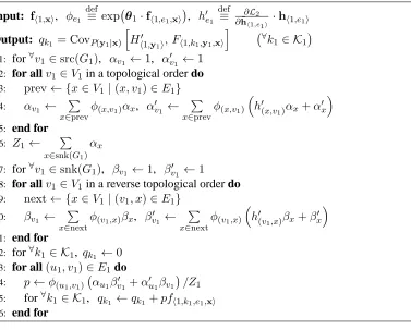
Algorithm 2 Forward-backward Algorithm for Calculating Feature Covariances
Input: f⟨1,x⟩, ϕe1 def
≡ exp(θ1·f⟨1,e1,x⟩
)
, h′e1 def≡ ∂L2 ∂h¯⟨1,e1⟩ ·
h⟨1,e1⟩
Output: qk1 = CovP(y1|x)
[
H⟨′1,y
1⟩, F⟨1,k1,y1,x⟩
] (
∀k
1 ∈ K1)
1: for∀v1 ∈src(G1), αv1 ←1, α′v1 ←1
2: for allv1 ∈V1in a topological order do
3: prev← {x∈V1 |(x, v1)∈E1}
4: αv1 ←
∑
x∈prev
ϕ(x,v1)αx, α′v1 ←
∑
x∈prev
ϕ(x,v1)
(
h′(x,v1)αx+α′x
)
5: end for
6: Z1← ∑
x∈snk(G1)
αx
7: for∀v1 ∈snk(G1), βv1 ←1, βv′1 ←1
8: for allv1 ∈V1in a reverse topological order do
9: next← {x∈V1|(v1, x)∈E1}
10: βv1 ←
∑
x∈next
ϕ(v1,x)βx, βv′1 ←
∑
x∈next
ϕ(v1,x)
(
h′(v
1,x)βx+β
′
x
)
11: end for
12: for∀k1 ∈ K1, qk1 ←0
13: for all(u1, v1)∈E1do
14: p←ϕ(u1,v1)(αu1βv′1 +α′u1βv1)/Z1
15: for∀k1 ∈ K1, qk1 ←qk1 +pf⟨1,k1,e1,x⟩
16: end for
sentences and 47377 words. The number of the POS label types is equal to 45. The number of the label types used in base-phrase chunking is equal to 23.
We compare the proposed method to two exist-ing sequence labelexist-ing methods as baselines. The POS labeler is the same in all the three methods used in this experiment. This labeler is a simple CRF and learned by ordinary optimization proce-dure. One baseline method is the 1-best pipeline method. A simple CRF model is learned for the chunking labeling, on the input sentences and the most likely POS label sequences predicted by the already learned POS labeler. We call this method “CRF + CRF.” The other baseline method has a CRF model for the chunking labeling, which uses the marginalized features offered by the POS la-beler. However, the parameters of the POS labeler are fixed in the training of the chunking model. This method corresponds to the method proposed in Bunescu (2008). We call this baseline “CRF + CRF-MF” (“MF” for “marginalized features”). The proposed method is the same as “CRF + CRF-MF”, except that the both labelers are jointly trained by the
CRF CRF CRF
+ CRF + CRF-MF +CRF-BP
POS labeling 95.6 (95.6) 95.8 Base-phrase 92.1 92.7 93.1
[image:8.612.88.465.60.363.2]chunking
Table 2: Experimental result (F-measure)
procedure described in Section 3. We call this pro-posed method “CRF + CRF-BP” (“BP” for “back propagation”).
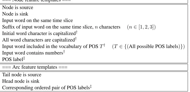
In “CRF + CRF-BP,” the objective function for joint learning (10) is not guaranteed to be convex, so optimization procedure is sensible to the initial con-figuration of the model parameters. In this experi-ment, we set the parameter values learned by “CRF + CRF-MF” as the initial values for the training of the “CRF + CRF-BP” method. Feature templates used in this experiment are listed in Table 1. Al-though we only described the formalization and op-timization procedure of the models with arc features, We use node features in the experiment.
[image:8.612.324.543.376.445.2]men-=== Node feature templates men-=== Node is source
Node is sink
Input word on the same time slice
Suffix of input word on the same time slice,ncharacters (n∈[1,2,3]) Initial word character is capitalized†
All word characters are capitalized†
Input word included in the vocabulary of POST† (T ∈ {(All possible POS labels)}) Input word contains numbers†
POS label‡
=== Arc feature templates === Tail node is source
Head node is sink
[image:9.612.119.516.54.246.2]Corresponding ordered pair of POS labels‡
Table 1: List of feature templates. All node features are combined with the corresponding node label (POS or chunking label) feature. All arc features are combined with the feature of the corresponding arc label pair. † features are instantiated on each time slice in five character window. ‡ features are not used in POS labeler, and marginalized as output features for “CRF + CRF-MF” and “CRF + CRF-BP.”
tioned. In Table 2, bold numbers indicate significant improvement over the baseline models with α = 0.05. From Table 2, the proposed method signifi-cantly outperforms two baseline methods on chunk-ing performance. Although the improvement on POS labeling performance by the proposed method “CRF + CRF-BP” is not significant, it might show that optimization procedure provides some form of backward information propagation in comparison to “CRF + CRF-MF.”
5 Conclusions
In this paper, we adopt the method to weight features on an upper sequence labeling stage by the marginal-ized probabilities estimated by the model on lower stages. We also point out that the model on an upper stage is considered to depend on the model on lower stages indirectly. In addition, we propose optimiza-tion procedure that enables the joint optimizaoptimiza-tion of the multiple models on the different level of stages. We perform an experiment on a real-world task, and our method significantly outperforms existing meth-ods.
We examined the effectiveness of the proposed method only on one task in comparison to just a few existing methods. In the future, we hope to compare our method to other competing methods like joint
learning approaches in terms of both accuracy and computational efficiency, and perform extensive ex-periments on various tasks.
References
M. Berz. 1992. Automatic differentiation as nonar-chimedean analysis. In Computer Arithmetic and
En-closure, pages 439–450.
R.C. Bunescu. 2008. Learning with probabilistic fea-tures for improved pipeline models. In Proceedings of
the 2008 Conference on Empirical Methods in Natural Language Processing, pages 670–679.
M. Collins and N. Duffy. 2002. New ranking algorithms for parsing and tagging: Kernels over discrete struc-tures, and the voted perceptron. In Proceedings of
the 40th Annual Meeting on Association for Compu-tational Linguistics, pages 263–270. Association for
Computational Linguistics.
G.F. Corliss, C. Faure, and A. Griewank. 2002.
Auto-matic differentiation of algorithms: from simulation to optimization. Springer Verlag.
J.R. Finkel, C.D. Manning, and A.Y. Ng. 2006. Solv-ing the problem of cascadSolv-ing errors: Approximate bayesian inference for linguistic annotation pipelines. In Proceedings of the 2006 Conference on Empirical
Methods in Natural Language Processing, pages 618–
626.
seg-menting and labeling sequence data. In Proceedings of
the Eighteenth International Conference on Machine Learning, pages 282–289.
Z. Li and J. Eisner. 2009. First-and second-order ex-pectation semirings with applications to minimum-risk training on translation forests. In Proceedings of the
2009 Conference on Empirical Methods in Natural Language Processing: Volume 1-Volume 1, pages 40–
51.
M.P. Marcus, M.A. Marcinkiewicz, and B. Santorini. 1993. Building a large annotated corpus of En-glish: The Penn Treebank. Computational linguistics, 19(2):330.
L.A. Ramshaw and M.P. Marcus. 1995. Text chunking using transformation-based learning. In Proceedings
of the Third ACL Workshop on Very Large Corpora,
pages 82–94. Cambridge MA, USA.
S. Sarawagi and W.W. Cohen. 2005. Semi-markov conditional random fields for information extraction.
Advances in Neural Information Processing Systems,
17:1185–1192.
C. Sutton, A. McCallum, and K. Rohanimanesh. 2007. Dynamic conditional random fields: Factorized proba-bilistic models for labeling and segmenting sequence data. The Journal of Machine Learning Research,
8:693–723.
B. Taskar, C. Guestrin, and D. Koller. 2003. Max-margin Markov networks. In Advances in Neural Information
Processing Systems 16.
RE Wengert. 1964. A simple automatic derivative evaluation program. Communications of the ACM,